Sage Journals: Discover world-class research

Abstract

The solution of the inverse kinematics of mobile manipulators is a fundamental capability to solve problems such as path planning, visual-guided motion, object grasping, and so on. In this article, we present a metaheuristic approach to solve the inverse kinematic problem of mobile manipulators. In this approach, we represent the robot kinematics using the Denavit–Hartenberg model. The algorithm is able to solve the inverse kinematic problem taking into account the mobile platform. The proposed approach is able to avoid singularities configurations, since it does not require the inversion of a Jacobian matrix. Those are two of the main drawbacks to solve inverse kinematics through traditional approaches. Applicability of the proposed approach is illustrated using simulation results as well as experimental ones using an omnidirectional mobile manipulator.

Keywords

Forward and inverse kinematics metaheuristic algorithms path tracking mobile manipulators mobile robotics

Introduction

Mobile manipulator is composed of one or more arm manipulators attached to a mobile platform. These kind of robots can be used to solve robot manipulation tasks and mobile navigation simultaneously. However, the combination of the degrees of freedom (DOFs) of the manipulator and the mobile platform commonly turns the mobile manipulator into a redundant robot. Cheong¹ transformed the mobile manipulator into a conventional manipulator via simulated virtual joints, and then kinematics models can be obtained as conventional fixed manipulators. The drawback of this approach is that it suffers from singularities configurations, since it requires the inversion of a Jacobian matrix to solve the inverse kinematics problems. Then, Huang and Tsai² and Tsai et al.³ introduced an approach to solve the inverse kinematics of omnidirectional mobile manipulators based on metaheuristic algorithms. However, this approach cannot be generalized to different mobile platform and manipulator structures. There are many works in mobile manipulator research, which solve the inverse kinematics of mobile manipulators^{4
–6}; however, these methods require the inversion of a Jacobin matrix or they cannot be generalized.

In this work, we are interested in a kinematic model of mobile manipulators, similar to conventional manipulators. To achieve this, we propose to represent the mobile platform with virtual joints.¹ In other words, the rotation angle of the platform can be represented by a virtual revolute joint and its translations with a virtual prismatic joint. Consequently, we can describe a kinematic model of the mobile manipulator using the Denavit–Hartenberg (DH) model as usually. For this reason, the proposed method becomes the inverse kinematics of mobile manipulator, which is an easier problem to solve.

Besides defining the model of mobile manipulators, we have to take into account that in general, mobile manipulators are redundant. Redundancy in robots occurs when they exceed the total DOFs that are strictly needed to perform a task. The solution of the inverse kinematics of redundant manipulators may result in multiple joint configurations to reach the same end-effector pose. Furthermore, the redundancy solutions may have singularities configurations that become the inverse kinematics to a problem difficult to solve.⁷ To overcome these problems, we propose to solve the inverse kinematics of redundant manipulators based on their kinematics equations. Because the proposed approach does not require the inversion of any Jacobian matrix and the forward kinematics always have a solution, there are no singular configurations as in the conventional methods for inverse kinematics.

The inverse kinematics of manipulators can be solved by minimizing an error function using some iterative process.^7,8 However, due to the complexity of mobile manipulator kinematics, it is necessary to search for no conventional methods to solve the inverse kinematics problem. Metaheuristic algorithms have been applied successfully to solve optimization problems in many researches areas.⁹ With respect to robotic researches, these algorithms are wisely used to solve the inverse kinematics and path-tracking problems,^{10

–13} motion planning,^14,15 visual servo control,^16,17 and mobile navigation.^{18

–23}

In this work, we propose the use of metaheuristic algorithms to solve the inverse kinematics of mobile manipulators as a constrained optimization problem. Initially, we define an objective function to minimize the error between the desired and the actual end-effector pose. The objective function takes into account the minimal movement between the previous and the actual joint configurations. To overcome the constrained problems, we use a penalty function to penalize all those manipulator configurations that violate the allowed joint boundary. Hence, the proposed approach estimates the feasible manipulator configuration needed to reach the desired end-effector pose.

The contribution of the proposed approach is the solution of the inverse kinematics of redundant mobile manipulators based on metaheuristic algorithms. Additionally, the proposed method does not suffer from singularities configurations as the result of the inverse kinematics. Finally, this approach can be applied to different combinations of mobile platforms and manipulator structures with n DOF.

This article is organized as follows: The next section will introduce the basic concepts about forward and inverse kinematics of robot manipulators. Then, the description of the considered metaheuristic algorithms is given. Next, we give a comprehensive description of the proposed approach. Later, the simulation and real experiments are presented, respectively. Finally, we give the conclusions.

Manipulator kinematics

Robot arm manipulators are composed of a series of rigid bodies called links.^24,25 These links are connected by joints, where the number of joints defines the total DOFs of the arm manipulator. Each joint is associated with an articulation to define a joint variable q. The forward kinematics computes the pose of the end effector, given the joint variable q. The vector q is defines as

q = {[\begin{matrix} q_{1} & q_{2} & q_{3} & \dots & q_{n} \end{matrix}]}^{T},

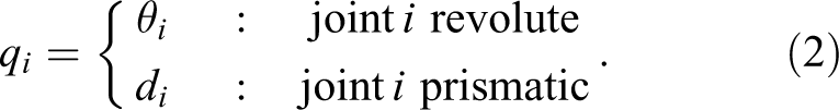
where each joint variable $q_{i} \in 1, 2, 3, \dots, n$ represents a joint position for the robot manipulator and n is the total number of DOF. In the case of a revolute joint, q_i is the angle of rotation, and in the case of a prismatic joint, q_i is the joint displacement

q_{i} = {\begin{matrix} θ_{i} & : & joint i revolute \\ d_{i} & : & joint i prismatic \end{matrix} .

The robot arm kinematic model of its links and joints forms a kinematic chain (see Figure 1). Based on its kinematic chain, the forward kinematic can be computed as

\begin{matrix} ^{0} T_{n} (q) =^{0} T_{1} (q_{1})^{1} T_{2} (q_{2})^{2} T_{3} (q_{3}) \dots^{n - 1} T_{n} (q_{n}) \\ = \prod_{i = 1}^{n}^{i - 1} T_{i} (q_{i}), \end{matrix}

Figure 1.

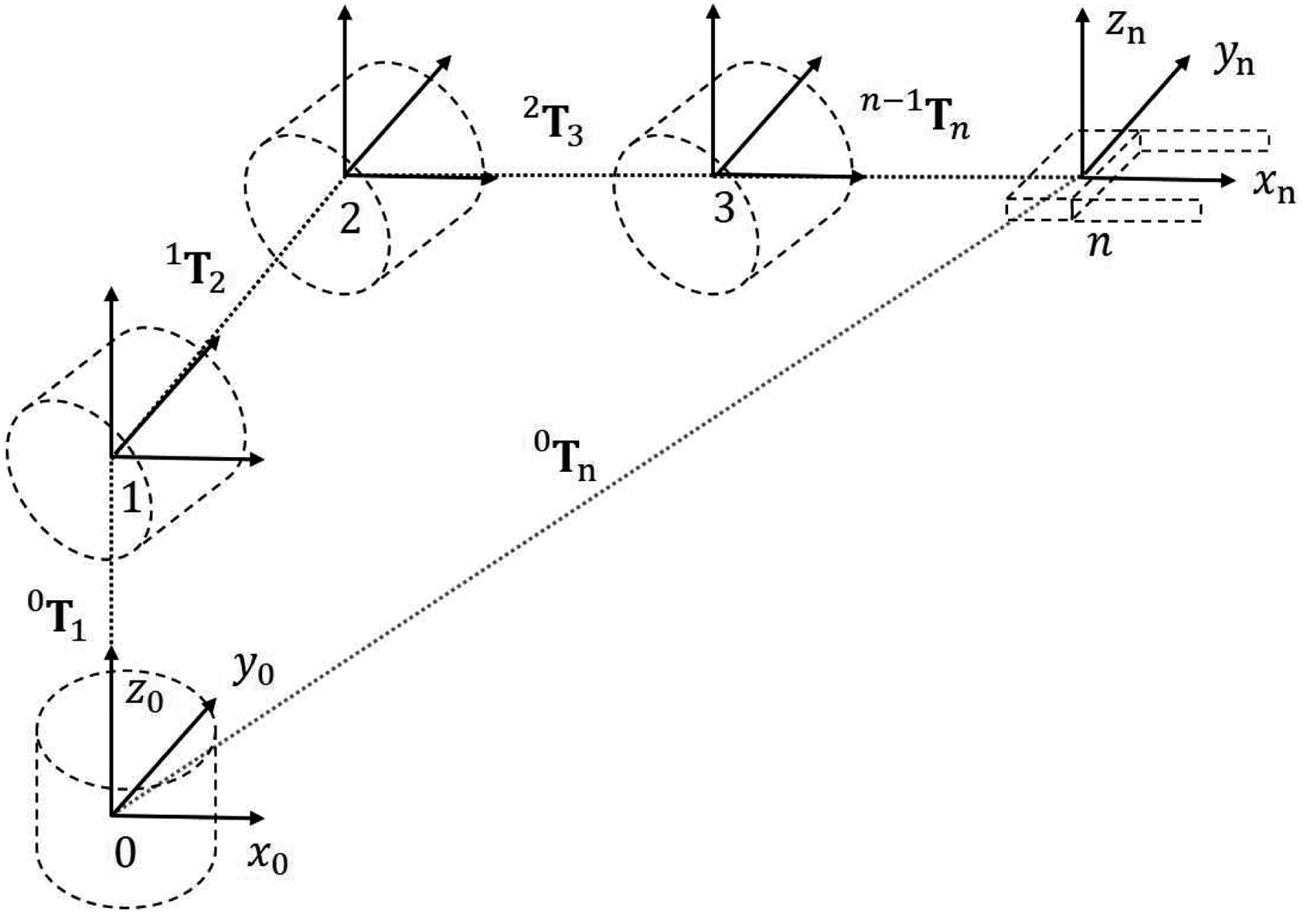
Kinematic chain of a manipulator. $^{i - 1} T_{i} (q_{i}) for i \in 1, 2, 3, \dots, n$ is the homogeneous matrix that represents the coordinate frame of the link i.

where $^{0} T_{n} (q)$ represents a homogeneous matrix that contains the end-effector pose. As seen in equation (3), each link i is represented by a homogeneous matrix $^{i - 1} T_{i} (q_{i})$ that transforms the frame attached to the link i − 1 into the frame link i, and this model can be described using the DH convention. Then, the homogeneous matrix $^{i - 1} T_{i} (q_{i})$ is expressed as the product of four basic transformations

^{i - 1} T_{i} (q_{i}) = T_{{rot}_{z}} (θ_{i}) T_{{trans}_{x}} (a_{i}) T_{{trans}_{z}} (d_{i}) T_{{rot}_{x}} (α_{i}) = [\begin{matrix} c θ_{i} & - s θ_{i} c α_{i} & s θ_{i} s α_{i} & a_{i} c θ_{i} \\ s θ_{i} & c θ_{i} c α_{i} & - c θ_{i} s α_{i} & a_{i} s θ_{i} \\ 0 & s α_{i} & c α_{i} & d_{i} \\ 0 & 0 & 0 & 1 \end{matrix}],

where θ_i is the joint angle, a_i is the link length, d_i is the link offset, and α_i is the link twist. These parameters are associated with the link and joint i. For brevity, the sin and cos operations are represented with the letters s and c, respectively. When a manipulator has a revolute joint, then the parameter θ_i in equation (4) becomes the joint variable and the other parameters remain constant. On the other hand, when the manipulator has a prismatic joint, then the parameter d_i becomes now the joint variable and the rest of the parameters remain constant.

When we compute the homogeneous matrix $^{i - 1} T_{i} (q_{i})$ using equation (4), we have the representation of the coordinate frame attached to the link i . This representation is expressed as

^{i - 1} T_{i} (q_{i}) = [\begin{matrix} n_{x} & o_{x} & a_{x} & p_{x} \\ n_{y} & o_{y} & a_{y} & p_{y} \\ n_{z} & o_{z} & a_{z} & p_{z} \\ 0 & 0 & 0 & 1 \end{matrix}] = [\begin{matrix} R_{i} & p_{i} \\ 0 & 1 \end{matrix}],

where R_i is a rotation matrix that represents the orientation of the respective frame i, and the vector p_i represents its Cartesian position.

The inverse kinematics consist in the computation of the joint variable q given the end-effector pose $^{0} T_{n}$ . The conventional approach consists in minimizing the error between an initial robot configuration $^{0} {\hat{T}}_{n} (\hat{q})$ and the desired end-effector pose $^{0} T_{n}$ .^7,26 However, an inconvenience of this approach is the singularities configurations. The solution of the inverse kinematics has a singularity configuration if there is no solution for the required Jacobian matrix $J^{- 1}$ . These singularities make the robot joint speed necessary to achieve a configuration and in consequence they become excessive. In order to overcome this problem, we propose the use of metaheuristic algorithms to solve the inverse kinematics based on its forward kinematics equations because the forward kinematics always has a solution. Moreover, the proposed approach does not require the inversion of any Jacobian matrix, and then it avoids singularities configurations.

More detailed information about forward and inverse kinematics can be found in the literature.^{7,24
–26}

Metaheuristic algorithms

Mobile manipulator is commonly named redundant robots, as the combination of the DOF of the mobile platform and the arm manipulator exceeds the total DOF needed to perform a task. The solution of the inverse kinematics for redundant robot results is a very difficult problem to solve by conventional approaches.¹¹ Traditional closed-form methods become difficult to implement for robots with particular geometric features. Furthermore, classical numerical methods may have singularities configurations as a result of the inverse kinematics. In this work, we propose the use of metaheuristic algorithms in order to solve the inverse kinematics of mobile manipulators as a constrained optimization problem. This approach does not suffer from singularities configurations, since it does not require a Jacobian matrix. Indeed, this approach uses the forward kinematics equations to solve the inverse kinematics problem with the advantage that forward kinematics always has a solution.

Metaheuristic algorithms have been commonly used for solving complex optimization problems such as classification, clustering, image processing, neural networks training, and others.⁹ With respect to robotic researches, several metaheuristic algorithms have been implemented to solve the inverse kinematics and path-tracking problems of robot manipulators. For example, the particle swarm optimization (PSO) has been used by different authors to solve the inverse kinematics for robot manipulators, including the redundant robots.^{27

–30} Some authors presented modifications to the PSO to overcome problems such as premature convergence. Ren et al.¹¹ introduced a hybrid approach for solving the inverse kinematics based on differential evolution (DE) and biogeography-based optimization (BBO); they called this method hybrid BBO (HBBO). They include a comparative study among DE, BBO, Genetic Algorithms (GA), and HBBO, where HBBO presents better results than the other algorithms. Then, Savsani et al.¹² present a comparative study which includes the artificial bee colony (ABC), BBO, gravitational search algorithm (GSA), cuckoo search (CS), firefly algorithm, bat algorithm, and teaching–learning-based optimization (TLBO). The authors concluded that ABC, TLBO, and CS performed better than the other algorithms for solving the trajectory planning for robot manipulators. The CS algorithm was also applied by Cai and Huang³¹ to solve the robot inverse kinematics. Next, in the study by Ayyildiz and Çetinkaya,¹⁰ the comparative study presented by the authors includes GSA, GA, PSO, and the quantum PSO (QPSO), where they concluded that QPSO is the most appropriate algorithm for the solution of the inverse kinematics.

Based on the previous references, in this work, we selected the CS, DE, HBBO, PSO, and TLBO algorithms to test the proposed approach. The DE algorithm is simple, robust, converge fast, and has a good balance between exploration and exploitation. DE is also easy to implement. For these reasons, we consider that the classic DE algorithm is good enough to solve the inverse kinematics of mobile manipulators. In the next subsection, we present a brief introduction to the DE algorithm.

Differential evolution

DE is a population-based algorithm that uses the mutation, crossover, and selection operations as a mechanism to improve its population members in every generation.³² The DE algorithm starts with a random initialization of the positions of a population of individuals whose positions represent a potential solution for the given problem. For each individual, an offspring or mutant vector is created using the weighted differences of parent members chosen randomly as follows

v_{i, G + 1} = x_{r 1, G} + F \cdot (x_{r 2, G} - x_{r 3, G}),

where $x_{r i, G}$ is the parent member with randomly chosen indexes $r_{1}, r_{2}, r_{3} \in 1, 2, 3, ..., N$ in each generation G, with N as the total number of individuals and $r_{1} \neq r_{2} \neq r_{3} \neq i$ with i as the actual index. The vector $v_{i, G + 1}$ is the mutant vector generated and $F \in [0, 2]$ is a constant factor that controls the amplification of the difference $x_{r 2, G} - x_{r 3, G}$ .

Using the crossover operation, the running vector $x_{r i, G}$ is mixed with the mutant vector $v_{i, G + 1}$ as follows

u_{j i, G + 1} = {\begin{array}{l} v_{j i, G + 1} & if (q_{1} (j) \leq C_{R}) or j = q_{2} (i) \\ x_{j i, G} & if (q_{1} (j) > C_{R}) and j \neq q_{2} (i) \end{array},

where $j = 1, 2, ..., D$ with D as the problem dimensionality, $q_{1} (j) and q_{2} (i)$ are random numbers and they are defined as $q_{1} \in [0, 1]$ which is the jth evaluation of a number, and $q_{2} (i) \in (1, 2, ..., D)$ is an index which ensures that $u_{i, G + 1}$ gets at least one element from $v_{i, G + 1}$ . The vector $u_{i, G + 1}$ is the trial vector and $C_{R} \in [0, 1]$ is the crossover constant.

Finally, if the trial vector $u_{i, G + 1}$ has a better fitness measure compared to the actual vector x_{i, G}, it is accepted as a new parent vector for the next generation; otherwise, the x_{i, G} vector is retained to the next generation. A review of DE and its parameters settings can be found in Gämperle et al.³³ Different modification to DE is also reported by Neri and Tirronen.³⁴

Description of the proposed approach

In this work, we propose to solve the inverse kinematics of mobile manipulator as a conventional fixed manipulator. Here, we describe a kinematic model of the mobile manipulator using the classical DH convention; therefore, the kinematics problems become easier to solve. In the proposed approach, we represent the mobile platform with virtual joints. The translation movement of the platform can be represented with prismatic joints; similarly, the rotation movements can be represented with revolute joints. Consequently, we obtain a kinematic chain using the DH model which contains the real and virtual joint of the mobile manipulator.

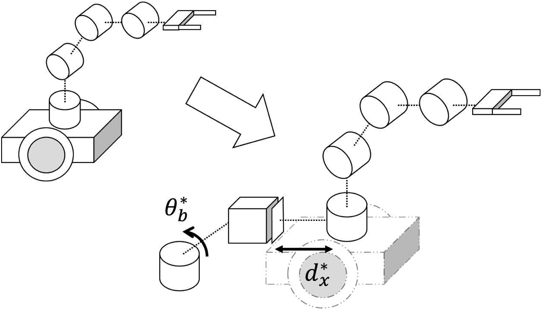
The mobile manipulators include different mobile platforms in combination with diverse manipulator structures. For example, Figure 2 illustrates an arm manipulator mounted in a differential-driven platform. Its equivalent model is also presented. The differential platform can be replaced with a virtual revolute joint $θ_{b}^{*}$ and a prismatic joint $d_{x}^{*}$ , which include the nonholonomic constraint. On the other hand, Figure 3 shows the combination of an arm manipulator with an omnidirectional platform. Its equivalent model is included as well. In this case, two virtual prismatic joints ( $d_{x}^{*} and d_{y}^{*}$ ) simulate the mobile translations and a virtual revolute joint ( $θ_{b}^{*}$ ) simulates its rotation. The proposed method can model other types of mobile platform and manipulator structures, and it is not limited to these examples. The next subsections give a detailed explanation about the description of the proposed approach for solving the inverse kinematics of mobile manipulators.

Figure 2.

Equivalent kinematic chain of a differential-driven mobile manipulator, where $θ_{b}^{*}$ represents a virtual join angle and $d_{x}^{*}$ a virtual joint displacement.

Figure 3.

Equivalent kinematic chain of an omnidirectional mobile manipulator, where $θ_{b}^{*}$ represents a virtual join angle and $d_{x}^{*} and d_{y}^{*}$ represent virtual joint displacements.

Fitness function formulation

We start by defining an error between the desired end-effector pose $^{0} T_{n}$ and the estimated end-effector pose $^{0} {\hat{T}}_{n}$ as follows:

T_{error} = ‖^{0} T_{n} -^{0} {\hat{T}}_{n} (\hat{q}) ‖,

where $^{0} T_{n},^{0} {\hat{T}}_{n} \in ℝ^{4 \times 4}, T_{error} \in ℝ, and \hat{q} \in ℝ^{n}$ are the estimated joint configurations with n as the total number of DOF and ‖ ⋅ ‖ is the Frobenius norm.

Then, we define an error between the previous joint position q_old and the estimated joint position $\hat{q}$ in order to minimize the motion of the manipulator. This error can be defined as

q_{error} = ‖ q_{old} - \hat{q} ‖,

where $q_{error} \in ℝ$ .

A fitness function can be defined as the weighted sum of the errors in equations (8) and (9) as follows

f (q_{old}, \hat{q}) = α T_{error} + β q_{error}

where α and β are weighting factors that scale the contribution of each term. Since the proposed approach solves the inverse kinematics of mobile manipulators as a constrained optimization problem, it is needed to include constrains in equation (10). In the literature, there are several methods to solve constrain optimization problems.³⁵ However, in this approach, we use a penalty function to overcome this problem.

In the case of mobile manipulators, constrains are defined as the manipulator joint limits and the works space assigned to the mobile platform. Given the lower q_l and upper q_l boundary, a penalty function g can be described as

g ({\hat{q}}_{j}) = {\begin{matrix} 0 & i f q_{l j} < {\hat{q}}_{j} < q_{u j} \\ 1 & otherwise, \end{matrix}

where j represents each joint variable in the kinematic chain. Finally, we include the penalty function (11) in equation (10) to obtain the proposed fitness function that handles constraints as

f' (q_{old}, \hat{q}) = f (q_{old}, \hat{q}) + γ \sum_{j = 0}^{n} g ({\hat{q}}_{j}),

where n represents the total number of DOF and γ scales the penalization term that is usually selected as a large constant. We recommend to use γ = 1000.

DE for solving the inverse kinematic problems

The proposed approach estimates the optimal joint configuration $\hat{q}$ needed to reach the desired end-effector pose $^{0} T_{n}$ . In DE algorithm, every individual contains a set of joint variables ${\hat{q}}_{i} with i \in 1, 2, 3, \dots, N$ , where N is the total number of individuals. The initialization of each individual is given by

{\hat{q}}_{i} = q_{l} + (q_{u} - q_{l}) r

where $r \in [0, 1]$ is a random number and q_l and q_u are the lower and upper joint boundary, respectively.

During the optimization process, the optimal joint configuration is found by solving the constrained optimization problem defined as

\begin{matrix} min f' (q_{old}, {\hat{q}}_{i}), \\ subject to q_{l} < {\hat{q}}_{i} < q_{u}, \end{matrix}

where every individual i evaluates the fitness function defined in equation (12). The iteration process ends when DE algorithm achieves the total number of iterations or when the evaluation of the fitness function reaches an allowed tolerance. In this case, the tolerance is given by a minimum value error between the desired end-effector position p and the desired position $\hat{p}$ .

The proposed algorithm based on DE is presented in Figure 4.

Figure 4.

Algorithm of the proposed approach based on DE. DE: differential evolution.

Simulation results

The aim of simulations is to test the behavior of the proposed approach solving the inverse kinematics of different mobile manipulators. A comparative study was performed in order to compare the performance among the CS, DE, HBBO, PSO, and TLBO. These metaheuristic algorithms have their own particular parameter settings, and they also have common parameter settings such as the population size, the number of iterations, and the tolerance. We decided to use a population size of 50 individuals, a maximum of 350 iterations, and an allowed tolerance of 0.001 m. The parameter settings for the standard CS algorithm were set to the probability factor p_a = 0.25 and the Levy flight factor α = 1.5. We based these settings as recommended in Savsani et al.,¹² and a similar configuration can also be found in Cai and Huang.³¹ We use the standard DE with the mutation strategy DE/ rand/1/ bin. Based on Gämperle et al.,³³ we fixed the amplification factor F and the crossover constant C_R to 0.6 and 0.9, respectively. For the HBBO algorithm, we fixed the maximum immigration rate I and the maximum emigration rate E to 1, the predetermined maximum mutation probability is ϕ_max = 0.05, and the scaling factor and crossover probability of the DE strategy are F = 0.6 and CR = 1.0, respectively. We based these parameter settings from Ren et al.¹¹ The PSO version used in this test includes the inertia weight modification. Here, the inertia weight is set to w = 0.8 as recommended by Shi and Eberhart,³⁶ and both the cognitive C₁ and social C₂ parameters are fixed to 2. Finally, the TLBO algorithm does not require any configuration parameter.¹² With respect to the weighting factors in the proposed fitness function, we recommend to use α = 1 and β = 0.1 giving priority to the T_error term.

In the simulations tests, we measured the execution time in seconds, the distance error p_error in meters, and the orientation error R_error and the displacement error q_error using the next equations

\begin{matrix} p_{error} = | | p - \hat{p} | | \\ R_{error} = | | R - \hat{R} | | \\ q_{error} = | | q - \hat{q} | |, \end{matrix}

where we obtain the values p and R from the desired end-effector pose $^{w} T_{n^{*}} and \hat{p} and \hat{R}$ from the estimated end-effector pose $^{w} {\hat{T}}_{n}$ . We notice that p_error is a Euclidean distance between the desired and the estimated position of the end-effector pose, R_error is Frobenius norm measure between the desired and the estimated orientation of the end effector, and q_error is a norm measure between the previous and the current estimated joint positions. The R_error and q_error errors do not have units of measurement.

The simulations were implemented in MATLAB. Every metaheuristic algorithm was run 100 times, and their results were illustrated using box plots. Box plots allow us to study distributional characteristics of a data set. This data distribution is represented into four groups divided by lines called quartiles. The middle box represents the central 50% of the data distribution, and its lower and upper boundary lines are at 25% and 75% of the data, respectively. The central line represents the median value. The two vertical lines extending from the middle box indicate the remaining 50% of the data distribution. They are called whiskers and they lower upper boundary lines, which are at the minimum and the maximum value of the data. Outlier is outside the middle box and the whiskers; these remaining values may be considered as noise in the data distribution. The intention of the use of box plots is to display graphically statistical variation in the proposed metaheuristic algorithm results. In the simulations, the execution time, position error, orientation error, and the displacement results are presented into box plots, where we are look for algorithm with smaller data distribution with lower value results and less quantities of outliers.

Inverse kinematic tests

In this experiment, we solve the inverse kinematics of a differential-driven platform in combination with four different manipulator structures. In this case, the joint variables are defined as $q = {[\begin{matrix} θ_{b}^{*} & d_{x}^{*} & θ_{1} & θ_{2} & \dots & θ_{m} \end{matrix}]}^{T}$ , where the virtual joints of the platform are represented with the joint variables $θ_{b}^{*} and d_{x}^{*}$ . The manipulator joints correspond to the variable θ_j with $j = 1, 2, \dots, m$ , where m is the total number of manipulator joints. The DH tables for the considered mobile manipulators with 6, 7, 8, and 9 DOFs are presented in Tables 1 to 4, respectively.

Table 1.

DH table for the differential-driven mobile manipulator with 6 DOF.^a

Joint	θ (rad)	d (mm)	a (mm)	α (rad)	Offset (rad)
1	$θ_{b}^{*}$	100	100	0	0
2	π/2	0	0	π/2	0
3	0	$d_{x}^{*}$	0	−π/2	0
4	θ ₁	150	50	π/2	−π/2
5	θ ₂	0	150	0	0
6	θ ₃	0	0	−π/2	0
7	θ ₄	150	0	0	0

DOF: degree of freedom; DH: Denavit–Hartenberg model.

^aJoints 1–3 represent the virtual joints of the platform and joints 4–7 the manipulator joints.

Table 2.

DH table for the differential-driven mobile manipulator with 7 DOF.^a

Joint	θ (rad)	d (mm)	a (mm)	α (rad)	Offset (rad)
1	$θ_{b}^{*}$	100	100	0	0
2	π/2	0	0	π/2	0
3	0	$d_{x}^{*}$	0	−π/2	0
4	θ ₁	150	50	π/2	−π/2
5	θ ₂	0	150	0	0
6	θ ₃	0	150	0	0
7	θ ₄	0	0	−π/2	0
8	θ ₅	150	0	0	0

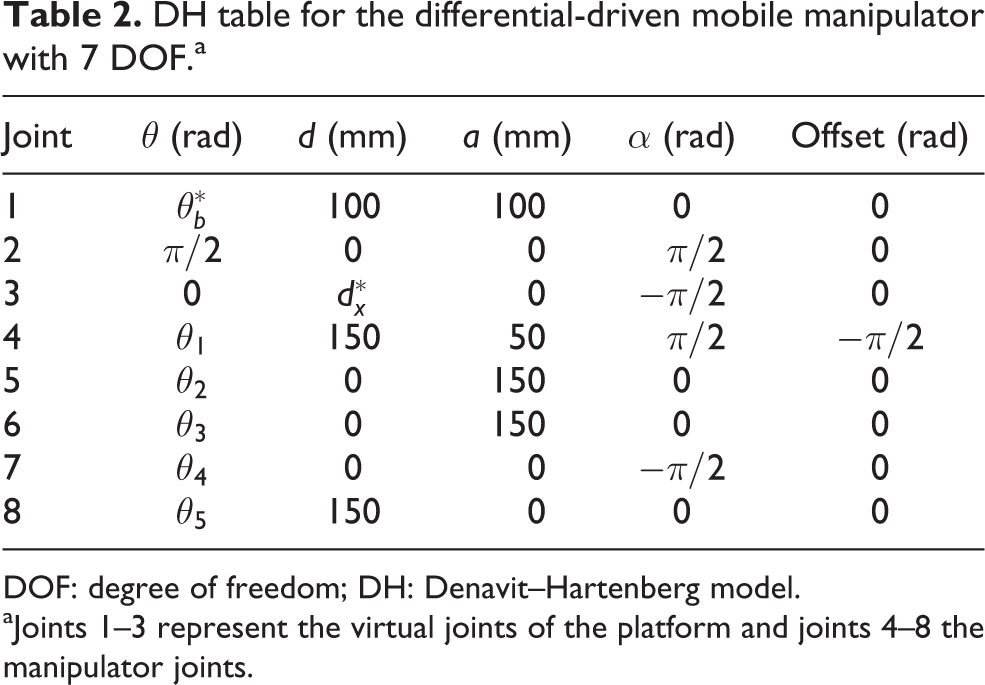
DOF: degree of freedom; DH: Denavit–Hartenberg model.

^aJoints 1–3 represent the virtual joints of the platform and joints 4–8 the manipulator joints.

Table 3.

DH table for the differential-driven mobile manipulator with 8 DOF.^a

Joint	θ (rad)	d (mm)	a (mm)	α (rad)	Offset (rad)
1	$θ_{b}^{*}$	100	100	0	0
2	π/2	0	0	π/2	0
3	0	$d_{x}^{*}$	0	−π/2	0
4	θ ₁	0	0	π/2	−π/2
5	θ ₂	0	150	0	0
6	θ ₃	150	50	−π/2	0
7	θ ₄	150	0	π/2	0
8	θ ₅	0	0	−π/2	0
9	θ ₆	0	0	0	0

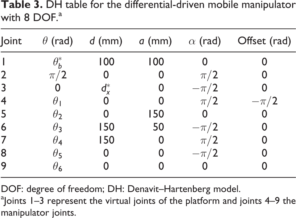
DOF: degree of freedom; DH: Denavit–Hartenberg model.

^aJoints 1–3 represent the virtual joints of the platform and joints 4–9 the manipulator joints.

Table 4.

DH table for the differential-driven mobile manipulator with 9 DOF.^a

Joint	θ (rad)	d (mm)	a (mm)	α (rad)	Offset (rad)
1	$θ_{b}^{*}$	100	100	0	0
2	π/2	0	0	π/2	0
3	0	$d_{x}^{*}$	0	−π/2	0
4	θ ₁	150	50	−π/2	−π/2
5	θ ₂	0	0	π/2	0
6	θ ₃	150	50	−π/2	0
7	θ ₄	0	0	π/2	0
8	θ ₅	150	50	−π/2	0
9	θ ₆	0	0	π/2	0
10	θ ₇	150	50	0	0

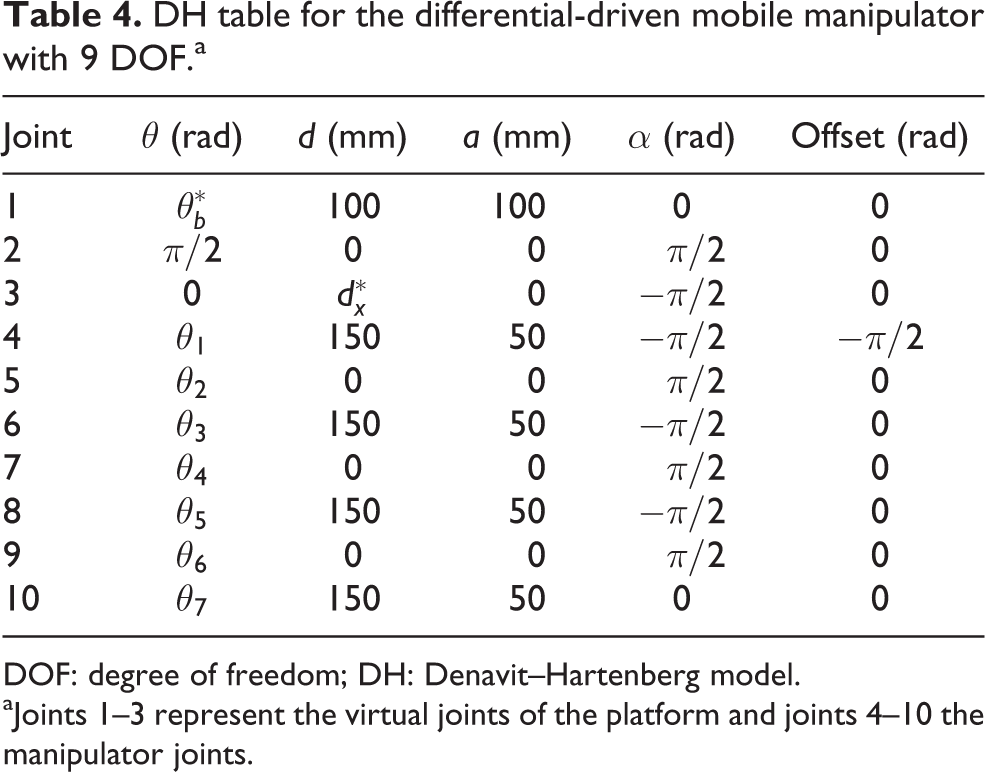
DOF: degree of freedom; DH: Denavit–Hartenberg model.

^aJoints 1–3 represent the virtual joints of the platform and joints 4–10 the manipulator joints.

In the inverse kinematics tests, the desired end-effector pose for all mobile manipulator was defined as

^{0} T_{n} = [\begin{matrix} 0 & 0 & 1 & 1.0 \\ 0 & - 1 & 0 & 1.0 \\ 1 & 0 & 0 & 0.5 \\ 0 & 0 & 0 & 1 \end{matrix}] .

The initial joint configuration for the considered mobile manipulators is given in Table 5. For every joint variable j, we established the next joint boundary

q_{l_{j}} = {\begin{matrix} - ϕ & : & joint j revolute \\ - 1.5 & : & joint j prismatic, \end{matrix}

q_{u_{j}} = {\begin{matrix} ϕ & : & joint j revolute \\ 1.5 & : & joint j prismatic, \end{matrix}

Table 5.

Initial joint configuration for the considered differential-driven mobile manipulators.

Joint	Mobile manipulator
Joint	6 DOF	7 DOF	8 DOF	9 DOF
1	0	−0.0614	−0.0103	−0.4852
2	0	−0.0894	0.3440	−0.1061
3	0	0.0625	1.3306	0.2062
4	0.5458	0.2026	0.6768	1.5
5	1.0247	0.1164	0.1204	1.3269
6	0	1.2528	1.7356	0.2825
7	—	0	1.7392	1.5882
8	—	—	−0.7831	0
9	—	—	—	0.2375

DOF: degree of freedom.

where $q_{l_{j}} and q_{u_{j}}$ are elements of the lower q_l and upper q_u joint boundary, respectively.

The simulation results for the 6-DOF differential-driven mobile manipulator are presented in Figure 5. In case of execution time included in Figure 5(a), DE had the best performance over the other algorithms, and its execution time performed below to 1 s. The CS, HBBO, and PSO algorithms had smaller data distribution, but they performed higher than 1.5 s. The HBBO algorithm also presents outlier results. On the other hand, TLBO had the largest data distribution. With respect to the position error in Figure 5(b), DE and TLBO performed below 1 mm of error, and they also have the smaller data distribution. In this case, PSO had the largest data distribution. About the orientation error in Figure 5(c), similar results are presented as in the position error case. Here, the DE and TLBO algorithms performed better than the others, and they present results below 0.01. Finally, Figure 5(d) shows the displacement error where CS, DE, and TLBO performed below 1.9 and they had a small data distribution; on the other hand, HBBO and PSO have a large data distribution.

Figure 5.

Simulation results for the 6-DOF differential-driven mobile manipulator. DOF: degree of freedom.

The simulation results for the 7-DOF differential-driven mobile manipulator are presented in Figure 6. In case of execution time included in Figure 6(a), DE had the best performance over the other algorithms, and its execution time performed below 1.5 s. The HBBO and TLBO have a large data distribution. In contrast, CS and PSO had small data distribution, but they performed above 1.8 s. With respect to the position error in Figure 6(b), DE and TLBO performed below 1 mm of error, and they also had the smaller data distribution. The PSO algorithm presents the largest data distribution. About the orientation error in Figure 6(c), the DE and TLBO algorithms performed better again than the others, and they present results below 0.01. Finally, Figure 5(d) shows the displacement error where CS, DE, and TLBO performed similar, but DE had the smallest data distribution; on the other hand, HBBO and PSO had the worst data distribution.

Figure 6.

Simulation results for the 7-DOF differential-driven mobile manipulator. DOF: degree of freedom.

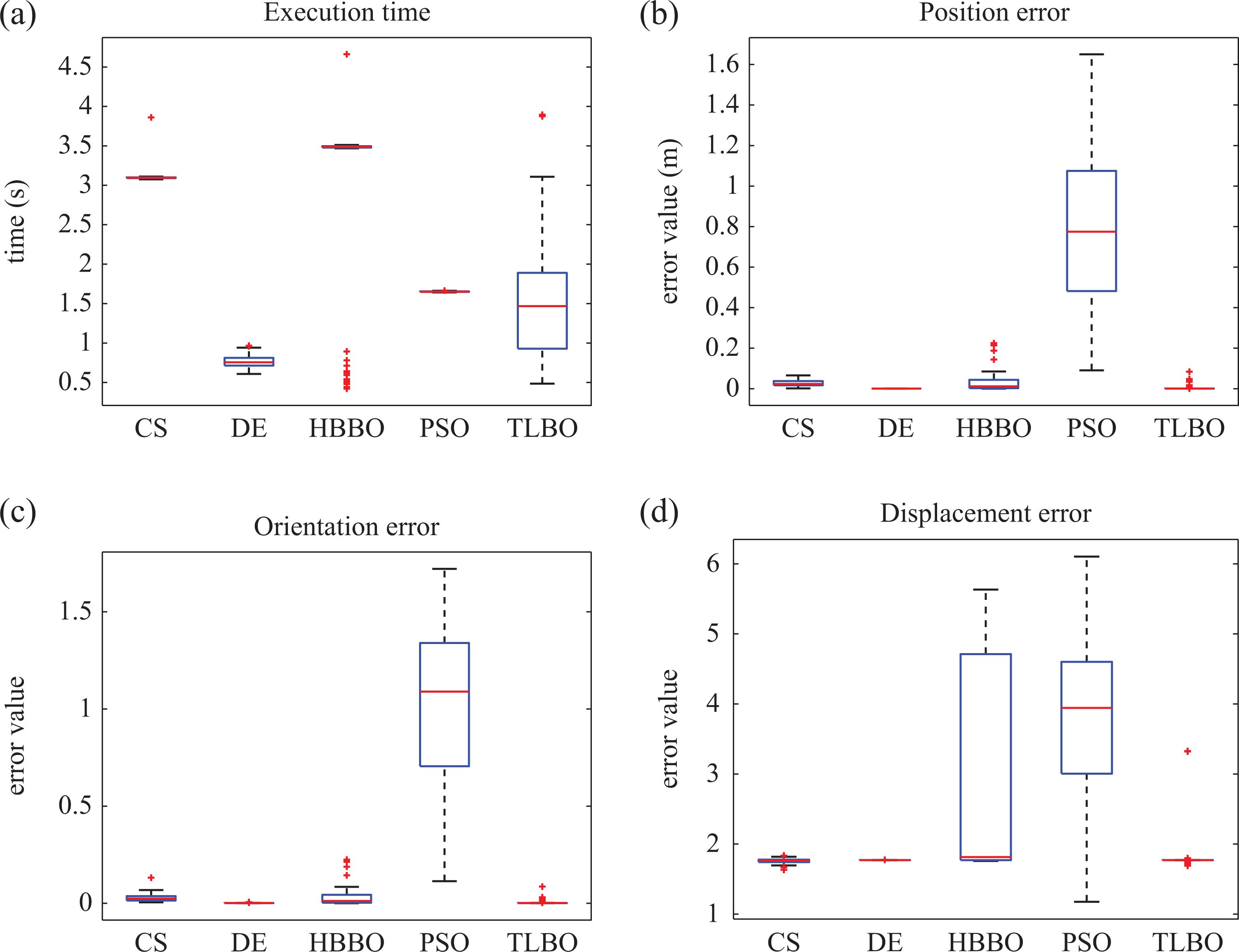
Figure 7 illustrates the simulation results for the 8-DOF differential-driven mobile platform. The execution time results in Figure 7(a) report that the CS, HBBO, and PSO had smaller data distribution, but DE had a best performance. The TLBO algorithm obtained a lot of outliers. The DE performs below 2.3 s. In contrast, TLBO had a large data distribution with results above 3 s. The distance error results in Figure 7(b) indicate that DE and TLBO had the best results, but DE performed below 1 mm. The CS, HBBO, and PSO algorithms presented higher distance errors. In the orientation results presented in Figure 7(c), DE and TLBO performed similar, and as a result they give errors below 0.02. The other algorithms presented greater errors. Finally, the displacement errors in Figure 7(d) indicate that DE outperformed other algorithms, with minimal displacement errors below 1.35.

Figure 7.

Simulation results for the 8-DOF differential-driven mobile manipulator. DOF: degree of freedom.

Figure 8 presents the results for the 9-DOF differential-driven mobile manipulator. The execution time results are given in Figure 8(a); DE and PSO have the best results, but PSO performed below 2 s. In contrast, the CS, HBBO, and TLBO algorithms performed above 3 s. The HBBO and TLBO had a lot of outlier results. In the case of the position error in Figure 8(b), DE and TLBO perform better than the other algorithms. They presented results below 10 mm. The other algorithms had larger results. With respect to orientation error in Figure 8(c), DE and TLBO had similar results. The orientation results are below 0.02. In this case, the PSO algorithm presented worst results. Finally, in Figure 8(d), the results of displacement errors are presented. The DE algorithm outperformed the others with error results below 2.5. The DE and the TLBO presented outlier results.

Figure 8.

Simulation results for the 9-DOF differential-driven mobile manipulator. DOF: degree of freedom.

In summary, according to the results of the inverse kinematics tests, the execution time increases with higher DOF mobile manipulators. The DE and the TLBO algorithm performed similar and better than CS, HBBO, and PSO, but DE proved to be faster than TLBO. Moreover, CS and HBBO performed similar in almost all cases. Furthermore, the results of the PSO algorithm proved that it does not solve the inverse kinematic problems correctly.

Figure 9 illustrates the results obtained by the proposed approach using the DE algorithm. In this figure, the old and the computed joint configurations are drawn, where q_old is the initial joint configurations and $\hat{q}$ is the obtained joints. These drawings intent to illustrate the minimal joint movement of the mobile manipulator.

Figure 9.

Inverse kinematics results for the proposed differential-driven mobile manipulators using the DE algorithm.

Path-tracking tests

In this test, we solve the path-tracking problem of an omnidirectional platform in combination with four different manipulator structures. In this case, the joint variables are defined as $q = {[\begin{matrix} d_{x}^{*} & d_{y}^{*} & θ_{b}^{*} & θ_{1} & θ_{2} & \dots & θ_{m} \end{matrix}]}^{T}$ , where the virtual joints of the platform are represented with the joint variables $d_{x}^{*}, d_{y}^{*}, and θ_{b}^{*}$ . The manipulator joints correspond to the variable θ_j with $j = 1, 2, \dots, m$ , where m is the total number of manipulator joints. The DH tables for the considered mobile manipulators with 7, 8, 9, and 10 DOF are presented in Tables 6 to 9, respectively. In these kinematic models, it is important to mention that it is necessary to rotate the kinematic chain $θ_{y} = π / 2$ about the y-axis for a propitiated kinematic model. We proposed to use the next equation to achieve the rotation

^{0} {T'}_{n} = T_{y}^{0} T_{n} (q) = [\begin{matrix} 0 & 0 & 1 & 0 \\ 0 & 1 & 0 & 0 \\ - 1 & 0 & 0 & 0 \\ 0 & 0 & 0 & 1 \end{matrix}]^{0} T_{n} (q),

Table 6.

DH table for the omnidirectional mobile manipulator with 7 DOF.^a

Joint	θ (rad)	d (mm)	a (mm)	α (rad)
1	0	$d_{x}^{*}$	0	−π/2
2	−π/2	$d_{y}^{*}$	0	π/2
3	$θ_{b}^{*}$	150	150	0
4	θ ₁	150	50	π/2
5	θ ₂	0	150	0
6	θ ₃	0	0	−π/2
7	θ ₄	150	0	0

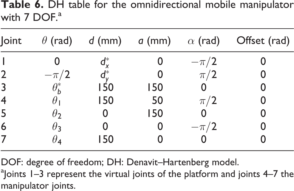
DOF: degree of freedom; DH: Denavit–Hartenberg model.

^aJoints 1–3 represent the virtual joints of the platform and joints 4–7 the manipulator joints.

Table 7.

DH table for the omnidirectional mobile manipulator with 8 DOF.^a

Joint	θ (rad)	d (mm)	a (mm)	α (rad)
1	0	$d_{x}^{*}$	0	−π/2
2	−π/2	$d_{y}^{*}$	0	π/2
3	$θ_{b}^{*}$	150	150	0
4	θ ₁	150	50	π/2
5	θ ₂	0	150	0
6	θ ₃	0	150	0
7	θ ₄	0	0	−π/2
8	θ ₅	150	0	0

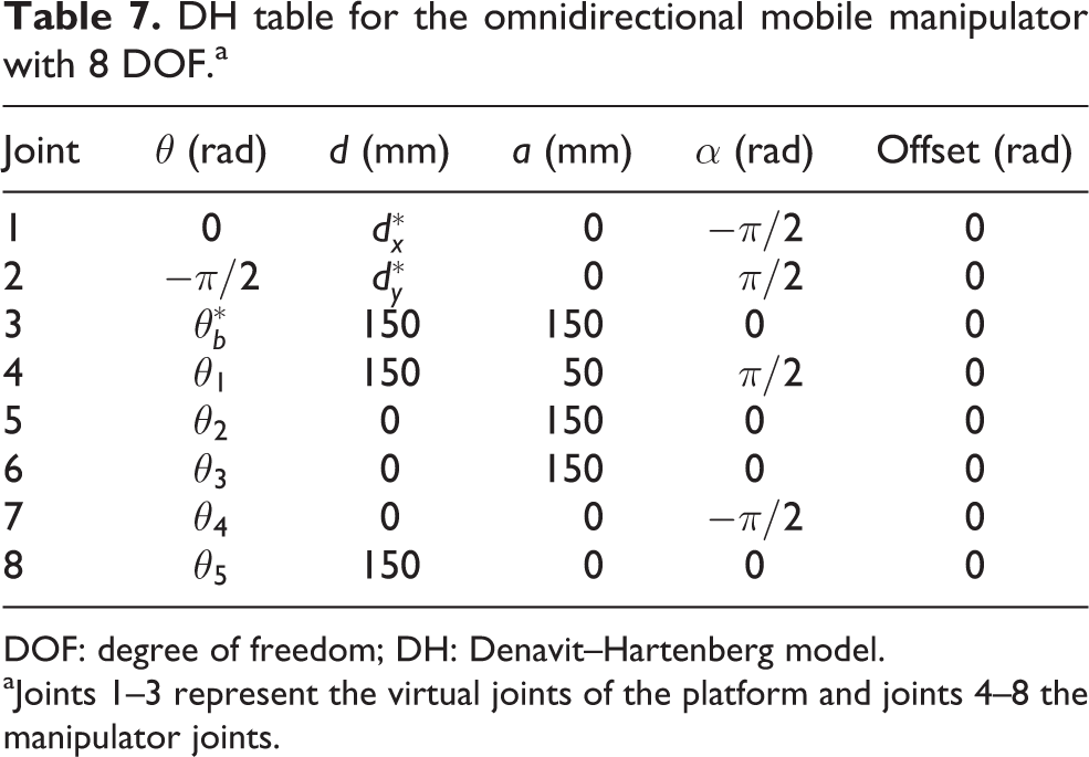
DOF: degree of freedom; DH: Denavit–Hartenberg model.

^aJoints 1–3 represent the virtual joints of the platform and joints 4–8 the manipulator joints.

Table 8.

DH table for the omnidirectional mobile manipulator with 9 DOF.^a

Joint	θ (rad)	d (mm)	a (mm)	α (rad)
1	0	$d_{x}^{*}$	0	−π/2
2	−π/2	$d_{y}^{*}$	0	π/2
3	$θ_{b}^{*}$	150	150	0
4	θ ₁	0	0	π/2
5	θ ₂	0	150	0
6	θ ₃	150	50	−π/2
7	θ ₄	150	0	π/2
8	θ ₅	0	0	−π/2
9	θ ₆	0	0	0

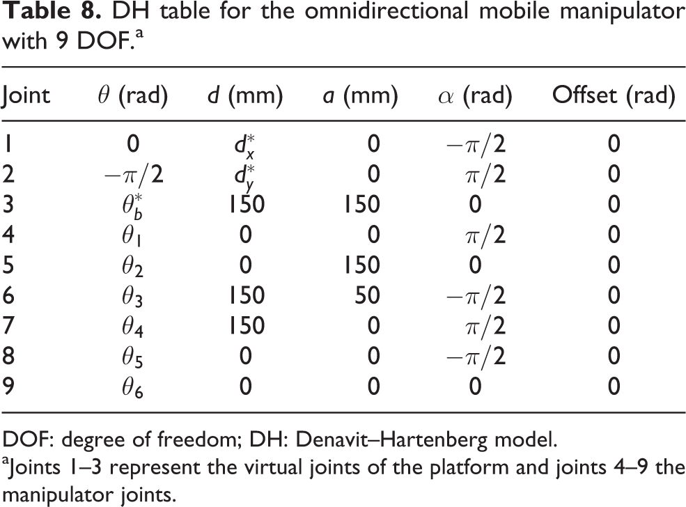
DOF: degree of freedom; DH: Denavit–Hartenberg model.

^aJoints 1–3 represent the virtual joints of the platform and joints 4–9 the manipulator joints.

Table 9.

DH table for the omnidirectional mobile manipulator with 10 DOF.^a

Joint	θ (rad)	d (mm)	a (mm)	α (rad)
1	0	$d_{x}^{*}$	0	−π/2
2	−π/2	$d_{y}^{*}$	0	π/2
3	$θ_{b}^{*}$	150	150	0
4	θ ₁	150	50	−π/2
5	θ ₂	0	0	π/2
6	θ ₃	150	50	−π/2
7	θ ₄	0	0	π/2
8	θ ₅	150	50	−π/2
9	θ ₆	0	0	π/2
10	θ ₇	150	50	0

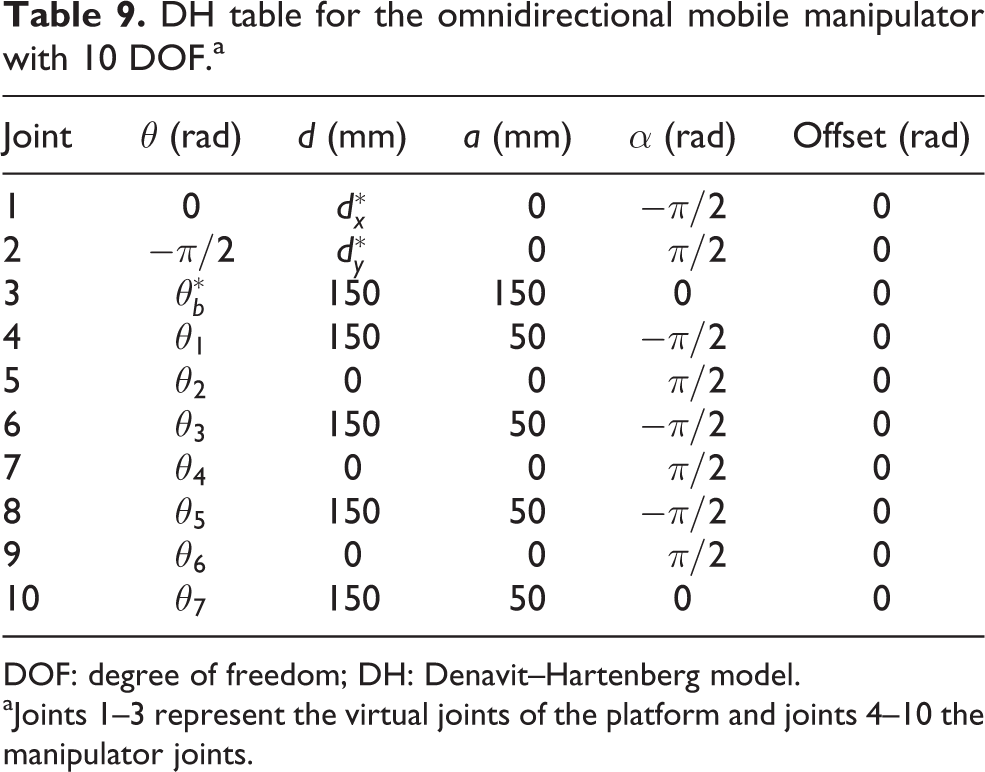
DOF: degree of freedom; DH: Denavit–Hartenberg model.

^aJoints 1–3 represent the virtual joints of the platform and joints 4–10 the manipulator joints.

where T_y is a transformation matrix that contains the rotation $R_{y} (θ_{y})$ . We use the $^{0} T_{n}^{'}$ homogeneous matrix to represent the end-effector pose of the omnidirectional mobile manipulators.

The path trajectory is given for a total number of O = 21 points with $^{0} T_{n}^{k}$ desired end-effector poses with $k = 1, 2, 3, \dots, O$ . To generate the translation position p_k in the desired trajectory, we propose to generate a trajectory based on the next equations

\begin{matrix} p_{x} = 1 \\ p_{y} = [- 1, 1] \\ p_{z} = C + A sin (B p_{y}), \end{matrix}

where the values A = 0.05, B = 10, and C = 0.3 were selected for the 7- and 9-DOF omnidirectional mobile manipulator. In case of 8- and 10-DOF mobile manipulators, we used A = 0.05, B = 10, and C = 0.04. With respect to the orientation of the desired end effector, the next rotation matrix is proposed to be used in the path trajectory

\begin{array}{l} R_{a} = [\begin{matrix} 0 & 0 & 1 \\ 0 & - 1 & 0 \\ 1 & 0 & 0 \end{matrix}] \end{array} \begin{array}{l} R_{b} = [\begin{matrix} 1 & 0 & 0 \\ 0 & 1 & 0 \\ 0 & 0 & 1 \end{matrix}], \end{array}

where R_a corresponds to the desired orientation for the 7-, 8-, and 10-DOF omnidirectional mobile manipulator and R_b corresponds to the 9-DOF mobile manipulator.

The initial joint configuration for the considered mobile manipulators is given in Table 10. The limit joint boundary for this test was selected according to equations (16) and (17).

Table 10.

Initial joint configuration for the considered omnidirectional mobile manipulators.

Joint	Mobile manipulator
Joint	6 DOF	7 DOF	8 DOF	9 DOF
1	0.0129	−0.0309	0.2284	0.2390
2	−0.0354	0.0201	−0.1713	−0.1359
3	0.2379	−0.1344	0.5207	−0.3803
4	−0.2379	0.1343	1.1459	0.9999
5	0.3403	0.2780	0.0460	1.5853
6	1.2305	0.1253	0.7143	1.1823
7	0	1.1675	1.5012	−0.5534
8	—	0	1.5048	1.4133
9	—	—	−0.7579	−0.2134
10	—	—	—	0.4903

DOF: degree of freedom.

The data distribution per each k point in the trajectory was averaged, and then box plots show the data distribution for all points in the trajectory. This means that a small data distribution in the position and orientation errors indicates a small variation in the estimated end-effector poses during the path trajectory.

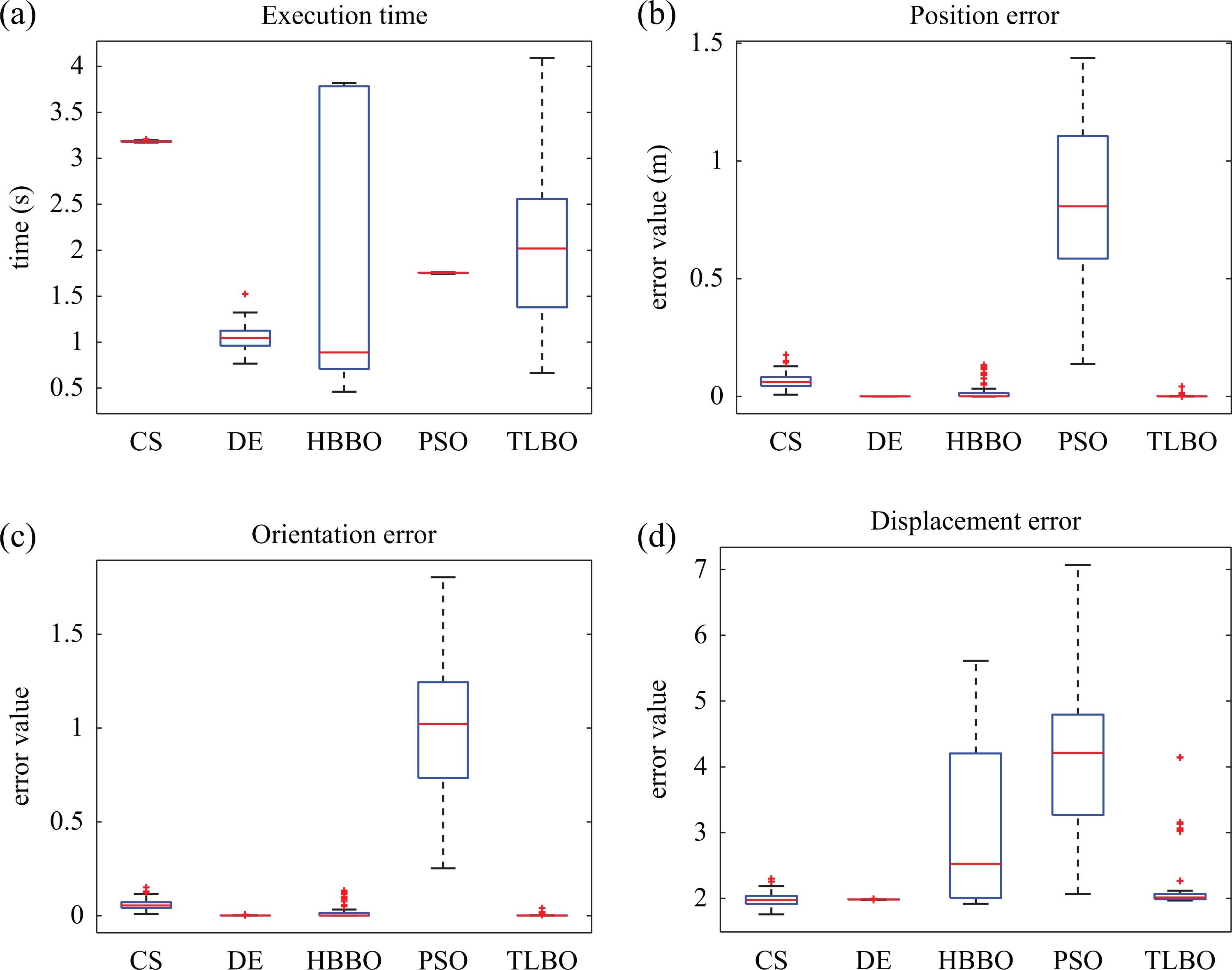
The simulation results for the 7-DOF omnidirectional mobile manipulator are presented in Figure 10. With respect to the execution time presented in Figure 10(a), DE and PSO had similar results, but DE had a smaller data distribution. Both algorithms performed below 30 s, while the other algorithms performed above 55 s. The position error results shown in Figure 10(b) indicate that DE outperformed the other algorithms with results below 1 mm. The other algorithms presented large results. In the case of the orientation error illustrated in Figure 10(c), DE and TLBO performed below 0.002. The CS, HBBO, and PSO had a large data distribution. Finally, the displacement error results are reported in Figure 10(d). The CS, DE, and TLBO had similar results, and their displacement errors are below 0.4. In contrast, the HBBO and PSO algorithms had larger error results.

Figure 10.

Simulation results for the 7-DOF omnidirectional mobile manipulator. DOF: degree of freedom.

In Figure 11, the simulation results for the omnidirectional mobile manipulators are reported. As we can see the execution time in Figure 11(a), the PSO algorithms performed better than the other, but DE presents a smaller data distribution. Both algorithms performed below 30 s. In the case of the position error results in Figure 11(b), DE outperformed the others with the smallest data distribution and errors below 1 mm. Larger results are presented by the other algorithms. With respect to the orientation error in Figure 11(c), similar results are presented as in the position error case, and DE performed better than the other algorithms with results below 0.02. Finally, the displacement error results are given in Figure 11(d), where CS, DE, and TLBO performed better than PSO and HBBO. These algorithms presented results below 0.25.

Figure 11.

Simulation results for the 8-DOF omnidirectional mobile manipulator. DOF: degree of freedom.

In Figure 12, the results for the 9-DOF omnidirectional mobile manipulators are given. The execution time results are illustrated in Figure 12(a), where PSO presented better results than the other algorithms. Its results are given below 30 s. In the case of the position error results reported in Figure 12(b) and the orientation error results reported in Figure 12(c), DE outperformed the other algorithms with results below 1 and 0.01 mm, respectively. Finally, the displacement error is illustrated in Figure 12(d). The DE and TLBO performed better than the other algorithms. The results are given below 0.22. The other algorithms presented errors above 0.42.

Figure 12.

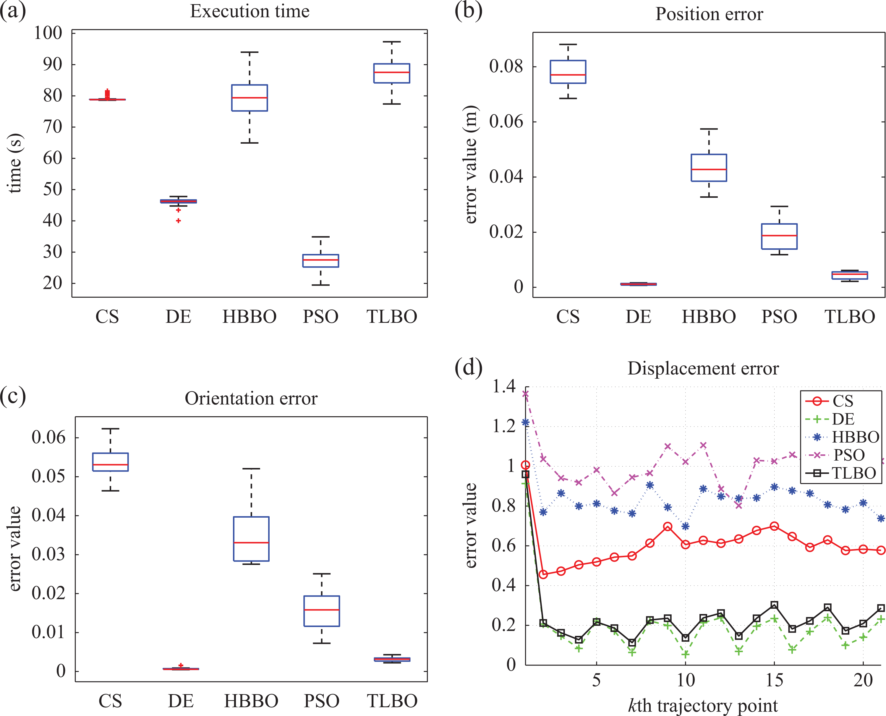
Simulation results for the 9-DOF omnidirectional mobile manipulator. DOF: degree of freedom.

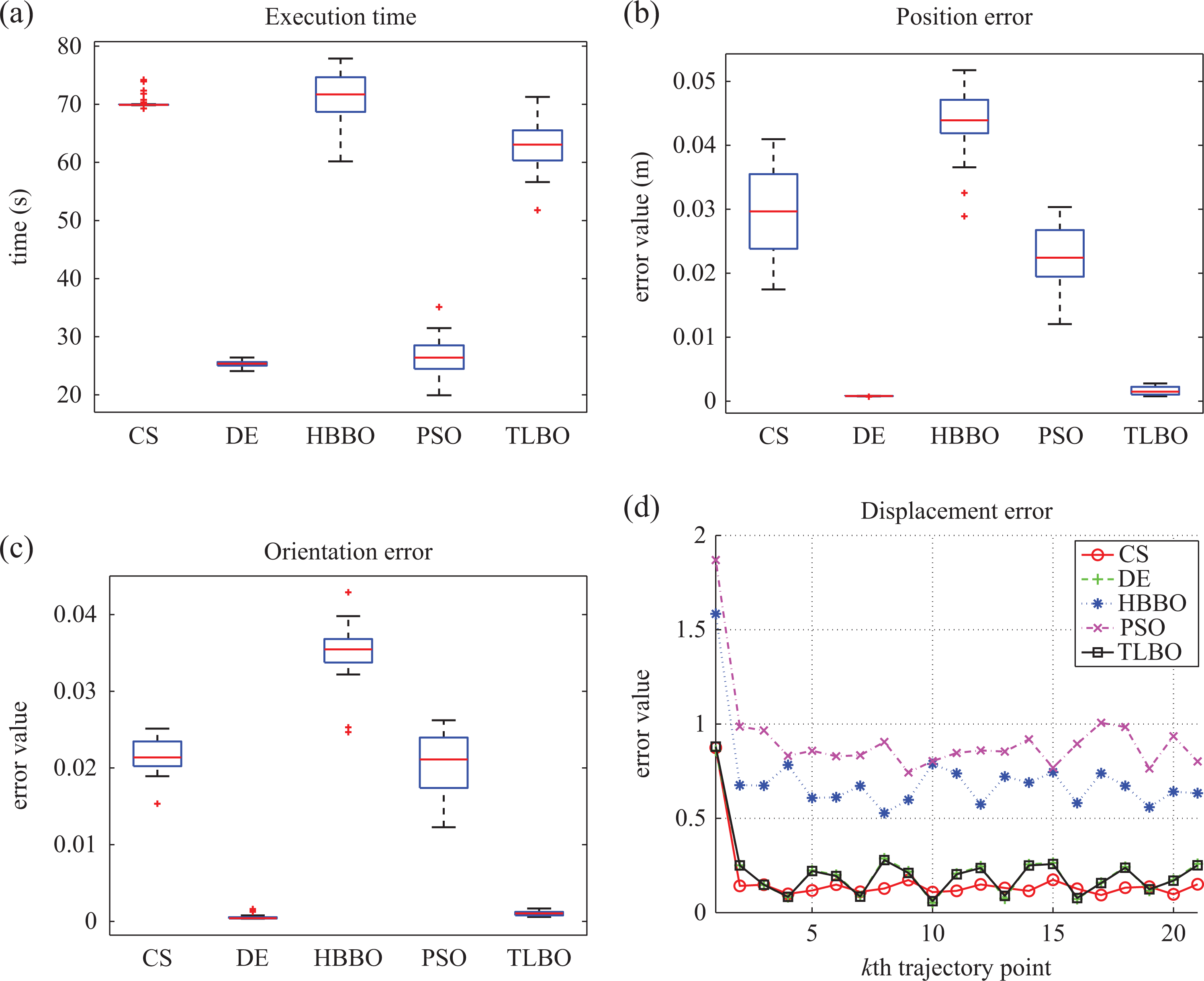
Next, the results for the 10-DOF omnidirectional mobile robot are given in Figure 13. The results for the execution time test are reported in Figure 13(a), and PSO presented better results below 40 s. The other algorithm results are given above 50 seconds. In the case of the position error results in Figure 13(b), the DE, PSO, and TLBO algorithms performed below 15 mm. With respect to the orientation error results in Figure 13(c), DE and TLBO had similar results, and the other algorithms presented larger errors. The DE and TLBO performed below 0.01. Finally, the graph in Figure 13(d) reported the results for the displacement errors. The DE outperformed the other algorithms with error results below 0.2.

Figure 13.

Simulation results for the 10-DOF omnidirectional mobile manipulator. DOF: degree of freedom.

Based on the results reported in the path-tracking test, DE performed better than the other algorithms in general. In this test, PSO shows to be able to solve the path-tracking problem with better results than the inverse kinematics test. The TLBO algorithms presented good results; however, the algorithm requires much more time to solve the path-tracking problems. The CS algorithm has the worst results with respect to time execution, position, and orientation errors.

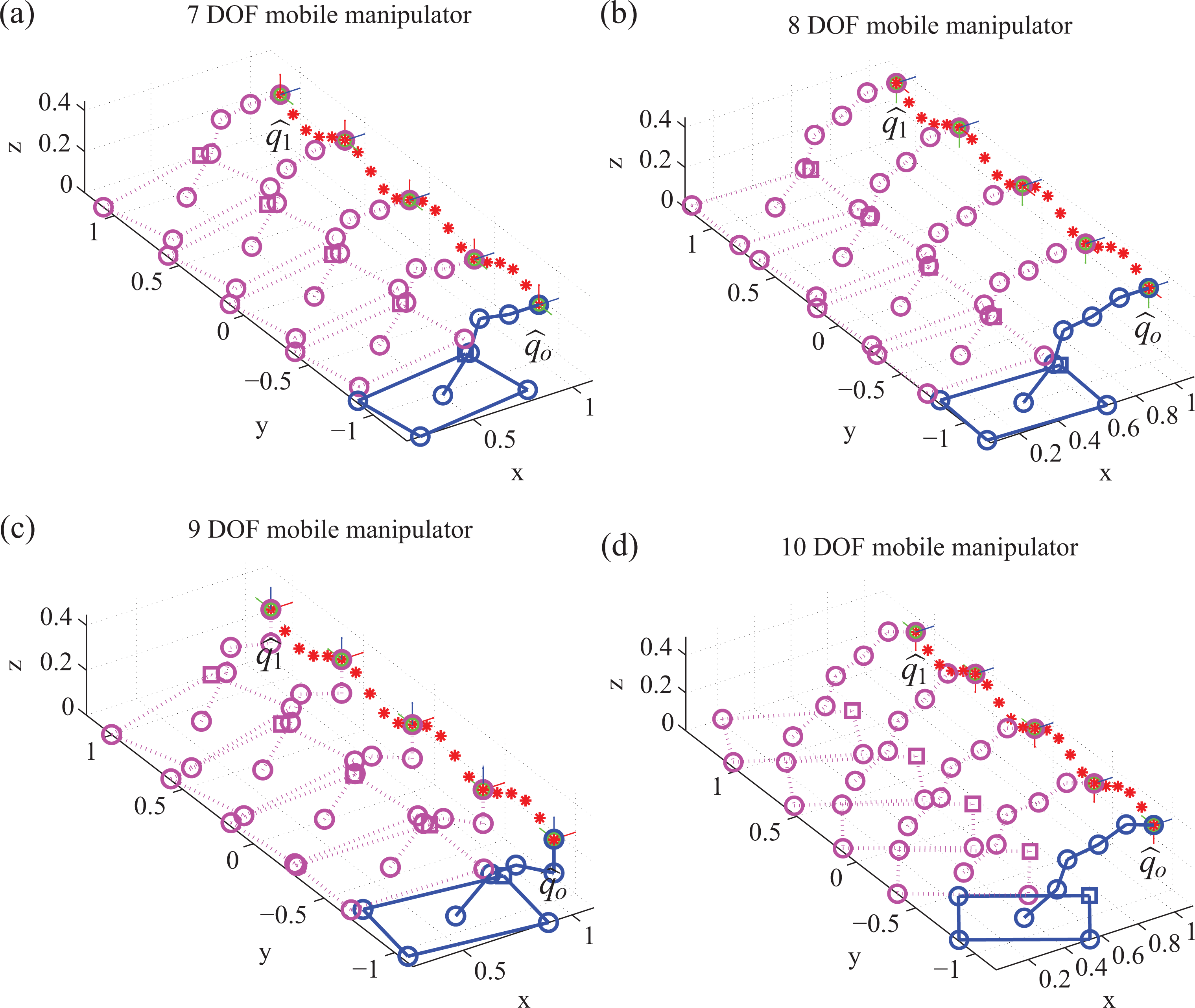
Figure 14 illustrates the minimal joint displacement results obtained by the proposed approach using the DE algorithm. In this figure, a few mobile manipulator configurations are drawn, where ${\hat{q}}_{1}$ is the first joint configuration and ${\hat{q}}_{O}$ is the last joint configuration obtained. These drawings intent to illustrate the minimal joint movement of the mobile manipulator.

Figure 14.

Path-tracking results for the proposed omnidirectional mobile manipulators using the DE algorithm. DE: differential evolution.

In summary, the performance of the DE algorithm is superior to the other algorithms in the solution of inverse kinematics and path-tracking problems. The DE algorithm requires less computational time and a minimal displacement movement of the robot articulations, in almost all cases. The DE also obtained the best position and orientation results over the other algorithms. For these reasons, DE is the most appropriated metaheuristic algorithm for solving the inverse kinematics problems of mobile manipulators.

The computational time results for the inverse kinematics and the path-tracking tests indicate that the proposed approach requires so much execution time to solve the inverse kinematics problems, in general. For these reasons, the proposed approach can be useful for solving the inverse kinematics in off-line applications. However, a DE parallel version may be an option to reduce this computational time,³⁷ and then the proposed approach might be applied in real-time applications.

Comparison tests

In this test, we perform a comparison study between the proposed approach and an existing inverse kinematics method.¹ The existing method consists in obtaining a kinematic model of mobile manipulators as conventional fixed manipulators. They transform the mobile manipulators into fixed manipulator via virtual joints. The authors also present an example of a 4-DOF car-like mobile manipulator using the mentioned method. However, this method suffers from singularities configurations, since it requires the inversion of a Jacobian matrix to solve the inverse kinematics problems via classical methods.

The mentioned 4-DOF car-like kinematic modeling obtained by the existing method can be found in the study by Cheong,¹ which is a simple planar two-link robot arm mounted on a car-like mobile platform. The inverse kinematics are solved by a classical iterative method (see Manipulator kinematics section). Because it is required, the inversion of a Jacobian matrix $J \in ℝ^{6, 4}$ , we proposed to use a fast computation algorithm for the Moore–Penrose pseudoinverse.³⁸ Finally, we used the following parameters for the given kinematic model: the links length $L_{1} = 0.5 m and L_{2} = 0.5 m$ and a link offset $h = 0.2 m$ .

In the proposed approach, the joint variables are given as $q = {[\begin{matrix} θ_{b}^{*} & d_{x}^{*} & θ_{1} & θ_{2} \end{matrix}]}^{T}$ , where the virtual joints of the platform are represented with the joint variables $θ_{b}^{*} and d_{x}^{*}$ . The manipulator joints correspond to the variables θ₁ and θ₂. The DH table for the 4-DOF car-like mobile manipulator is presented in Table 11.

Table 11.

DH table for the car-like mobile manipulator with 4 DOF.^a

Joint	θ (rad)	d (mm)	a (mm)	α (rad)	Offset (rad)
1	$θ_{b}^{*}$	0	0	0	0
2	π/2	0	0	π/2	0
3	0	$d_{x}^{*}$	200	−π/2	0
4	θ ₁	0	500	0	0
5	θ ₂	0	500	0	−π/2

DOF: degree of freedom; DH: Denavit–Hartenberg model.

^aJoints 1–3 represent the virtual joints of the platform and joints 4 and 5 the manipulator joints.

According to the results of the previous simulations, we use the DE algorithm in this test. The standard version of DE was used with the DE/rand/1/ bin mutation strategy, the amplification factor F = 0.6, and the crossover constant C_R = 0.9. We also used 100 individuals, 350 iterations, and an allowed tolerance of 0.0001 m. In this test, we performed four trajectories tracking. These trajectories are given by the following equations:

\begin{array}{l} x = 0.7 - 0.6 k \\ y = 1 - 2 k, \end{array}

\begin{array}{l} x = 0.2 + 0.05 sin (10 y) \\ y = [- 1, 1], \end{array}

\begin{array}{l} r = 0.3 + 0.1 cos (3 θ) \\ x = 0.5 + r cos (θ) \\ y = r sin (θ), \end{array}

\begin{array}{l} x = 0.5 + 0.2 cos (θ) \\ y = - 0.2 + 0.2 sin (θ), \end{array}

where k and θ determine each point (x, y) in the trajectory. Equations (19) and (20) correspond to the trajectory tests 1 to 4, respectively.

We have to mention that for the compared methods, joint limits are not considered, and we did not solve the orientation problem due to the kinematic limitations of the considered 4-DOF car-like mobile manipulator. In the proposed approach, T_error in equation (8) can be written as

T_{error} = | | p_{d} - \hat{p} | |,

where p_d is the desired end-effector position and $\hat{p}$ is the estimated position. The position error result T_error is a Euclidean distance error; therefore, this error should be as small as possible.

Figure 15 shows the results for the position errors of the compared methods. As we can see, at some points of the four trajectories, the classical method gives large errors such as 640 mm in trajectory 1, 115 mm in trajectory 2, and 270 and 160 mm in trajectory 4. These errors may occur when the classical method computes the inverse kinematics near to a singular configuration. In contrast, the proposed approach gives better results. Most appropriated results for the position error results are given in Table 12, where the proposed approach outperformed the classical method in all the trajectory tests. The proposed approach performed below an average position error of 0.01 mm and a standard deviation below 0.00003.

Figure 15.

Position error results for the classical and the proposed inverse kinematics methods. (a) Trajectory 1. (b) Trajectory 2. (c) Trajectory 3. (d) Trajectory 4.

Table 12.

Position error results for the classical and the proposed inverse kinematics methods.

Trajectory	RMS		STD
Trajectory	Classic	Proposal	Classic	Proposal
1	0.137522	0.000069	0.137244	0.000025
2	0.025621	0.000070	0.024172	0.000026
3	0.048261	0.000068	0.048227	0.000024
4	0.029219	0.000066	0.029096	0.000024

RMS: root mean square; STD: standard deviation.

Bold values indicates the best result.

Figures 16 and 17 present the results of a joint displacement for the classical method and the proposed approach, respectively. The classical method reported abrupt chances in the joint displacement values because of the singularity configurations. On the other hand, the results of the proposed method reported smooth trajectory in the four trajectory tests.

Figure 16.

Joint displacement results for the classical inverse kinematics method. (a) Trajectory 1. (b) Trajectory 2. (c) Trajectory 3. (d) Trajectory 4.

Figure 17.

Joint displacement results for the proposed inverse kinematics method. (a) Trajectory 1. (b) Trajectory 2. (c) Trajectory 3. (d) Trajectory 4.

To conclude, the classical method suffers from singularities configurations, and at some points of the given trajectories, the inverse kinematic task fails. In contrast, the proposed approach overcomes singularities configurations because it is not required the inversion of a Jacobian matrix in this method.

Experimental results

The aim of the real experiments is to test the behavior of the proposed approach for solving the path-tracking problem of an omnidirectional mobile manipulator. Given the results of simulation experiments, we use the DE algorithm to solve the path-tracking problem. The standard version of DE was used with the DE/rand/1/bin mutation strategy, the amplification factor F = 0.6, and the crossover constant C_R = 0.9, similar to the simulation case. We also used 100 individuals, 500 iterations, and an allowed tolerance of 0.0001 m.

The proposed omnidirectional mobile manipulator is the KUKA Youbot illustrated in Figure 18. The DH parameters for this robot which include the mobile platform virtual joints are presented in Table 13. In this case, the joint variables are given as $q = {[\begin{matrix} q_{base}^{T} & q_{arm}^{T} \end{matrix}]}^{T}$ which represent an 8-DOF mobile manipulator, where $q_{base} = {[\begin{matrix} d_{x}^{*} & d_{y}^{*} & θ_{b}^{*} \end{matrix}]}^{T}$ represents the platform virtual joint variables and $q_{arm} = {[\begin{matrix} θ_{1} & θ_{2} & θ_{3} & θ_{4} & θ_{5} \end{matrix}]}^{T}$ the manipulator joint variables. The joint boundary is given as follows:

\begin{array}{l} q_{l} = [- 1.5 - 1.5 - 3.1416 - 2.9496 \\ {0 2.6354 - 0.2182 - 2.9234]}^{T} \\ q_{u} = [1.5 1.5 3.1416 2.9496 \\ {2.7053 - 2.5482 3.3598 2.9234]}^{T} . \end{array}

Figure 18.

KUKA Youbot, omnidirectional mobile platform with a 5-DOF manipulator. DOF: degree of freedom.

Table 13.

DH table for the KUKA Youbot omnidirectional mobile manipulator with 8 DOF.^a

Joint	θ (rad)	d (mm)	a (mm)	α (rad)
1	0	$d_{x}^{*}$	0	−π/2
2	−π/2	$d_{y}^{*}$	0	π/2
3	$θ_{b}^{*}$	140	151	0
4	θ ₁	147	33	π/2
5	θ ₂	0	155	0
6	θ ₃	0	135	0
7	θ ₄	0	0	π/2
8	θ ₅	217.5	0	0

DOF: degree of freedom; DH: Denavit–Hartenberg model.

^aJoints 1–3 represent the virtual joints of the platform and joints 4–8 the manipulator joints.

The path trajectory was generated with O = 200 total points. The desired position p_k and orientation R of the end effector $^{0} T_{n}^{k}$ were assigned based on the next equations

\begin{array}{l} R = [\begin{matrix} 0 & 0 & 1 \\ 0 & - 1 & 0 \\ 1 & 0 & 0 \end{matrix}] \end{array} \begin{array}{l} p_{x} = 0.5 \\ p_{y} = [- 1, 1] \\ p_{z} = 0.5 + 0.05 sin (5 p_{y}) . \end{array}

Finally, the initial joint configuration was fixed to q = 0.

The proposed approach was implemented using C++ and ROS environment. There is an existing ROS component for the KUKA Youbot to access to the manipulator and the mobile platform hardware. We used the integrated controller for the manipulator. On the other hand, we implemented a proportional-derivative controller for the mobile platform. The kinematics and control techniques for mobile platform can be found in the literature.^{39
–41}

It was needed to define an offset q_offset in order to use the integrated manipulator controller. This offset is defined as

q_{offset} = {[\begin{matrix} 2.9496 & 2.7053 & - 2.5482 & 3.3598 & 2.9234 \end{matrix}]}^{T}

Then, we computed the joint variable q_ctrl needed for the manipulator controller as follows:

q_{ctrl} = - {\hat{q}}_{arm} + q_{offset} .

Figure 19 presents the results for the 1–4joints in the joint variable $\hat{q}$ . The joints 1–3 correspond to the mobile platform and joint 4 to the first arm joint. On the other hand, Figure 20 illustrates the results for five to eight joints that correspond to the manipulator joints. The computed results indicate the joint variable results by the proposed approach, and the real joint variables indicate real values acquired from the KUKA Youbot sensors. In the case of the manipulator joint results (see Figure 19(d) and Figure 20), the values of computed joints and real joints are very similar. In contrast, the real joint values for the Youbot platform have a small variation (see Figure 19(a) to (c)). However, the computed joint results by the proposed approach reported a smooth trajectory for the given task.

Figure 19.

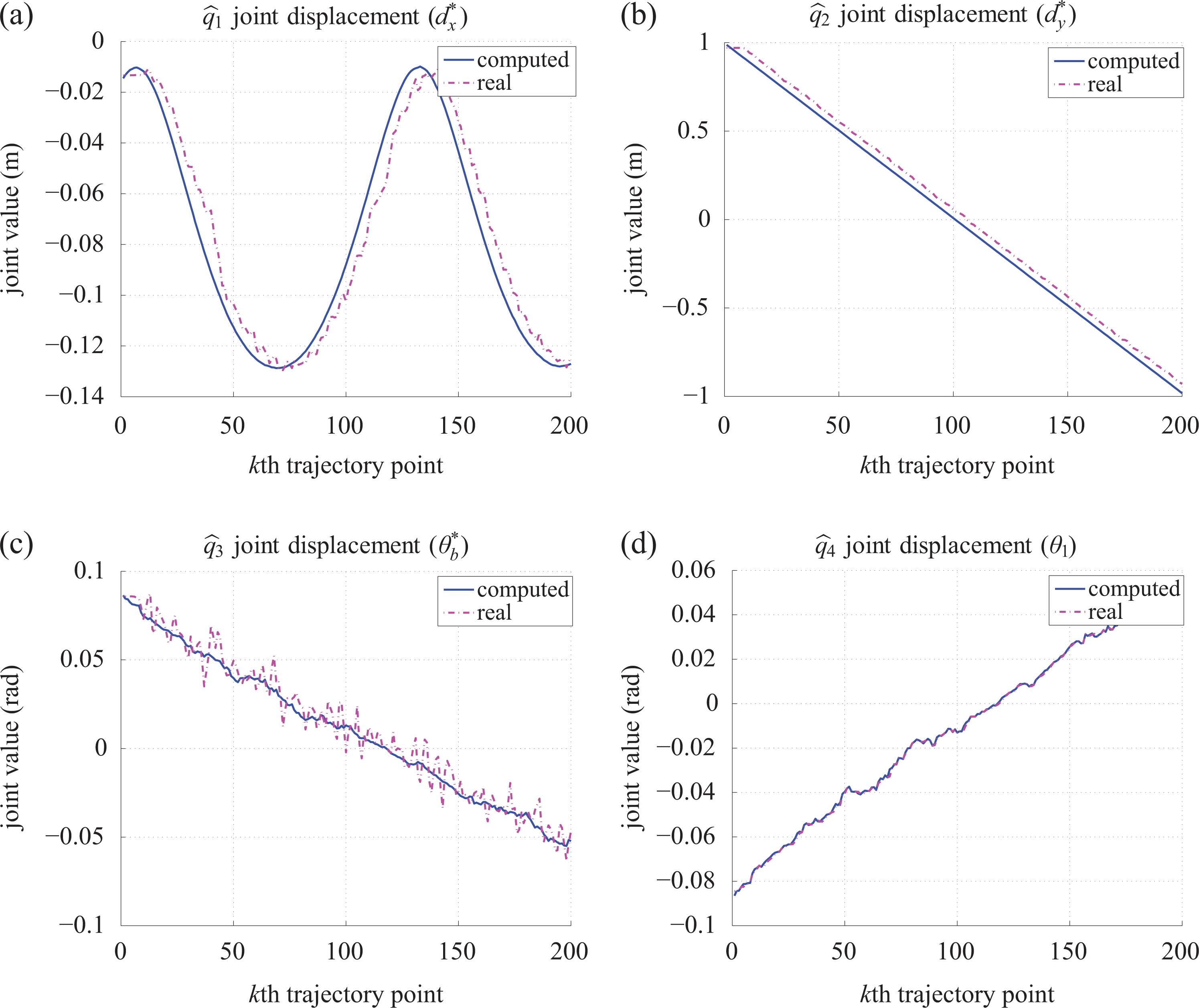
Joint displacement results for the KUKA Youbot. The reported results correspond to the one to four joints in the joint variable $\hat{q}$ .

Figure 20.

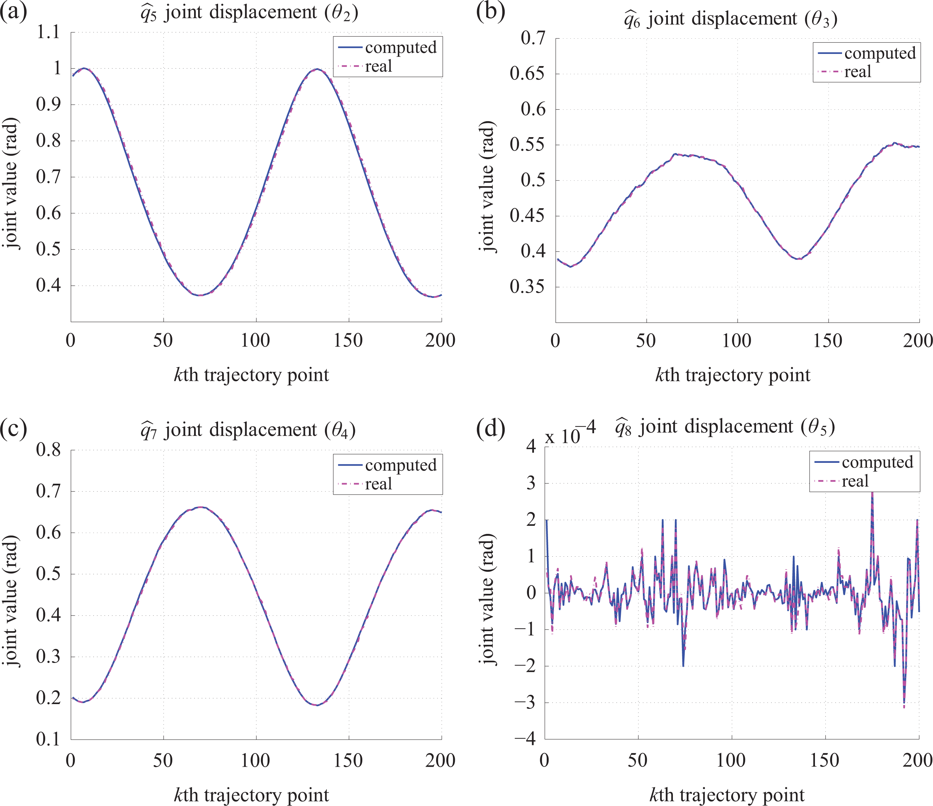
Joint displacement results for the KUKA Youbot. The reported results correspond to the five to six joints in the joint variable $\hat{q}$ .

Based on the result presented in this test, the proposed approach solves successfully the path-tracking problem for the KUKA Youbot omnidirectional mobile manipulator. Moreover, a better base controller should be used for the mobile platform; in contrast, the integrated manipulator controller reported good results. Finally, the implementation of the path-tracking problem for the KUKA Youbot omnidirectional mobile manipulator is illustrated in Figure 21.

Figure 21.

KUKA Youbot solving a path-tracking task.

Conclusions

In this article, we introduced an approach for solving the inverse kinematics of mobile manipulators based on metaheuristic algorithms. Simulation and real experiments were performed to prove the effectiveness of the proposed approach. The metaheuristic algorithms included in the simulations were the CS, DE, HBBO, PSO, and TLBO. Additionally, different redundant mobile manipulators such as the differential-driven and omnidirectional mobile manipulators were considered in simulations. In the experiments, the KUKA Youbot omnidirectional mobile manipulator was considered as well. From simulations and real experiment results, the results of the DE algorithm proved to be superior than the other algorithms with respect to the minimum computational time, a minimum error in the position and orientation for the desired end-effector pose, and the minimal joint movement for the considered mobile manipulators. The HBBO provided good results but with a higher computational cost. The CS and PSO algorithms reported poor results; consequently, these algorithms are not recommended for solving the inverse kinematics of mobile manipulators. In conclusion, the proposed approach can solve the inverse kinematics of mobile manipulators effectively, and in real time, the robots can have different configurations including redundant robots.

Footnotes

Acknowledgement

The authors would like to thank the support of CONACYT México and the University of Guadalajara.

Declaration of conflicting interests

The author(s) declared no potential conflicts of interest with respect to the research, authorship, and/or publication of this article.

Funding

The author(s) disclosed receipt of the following financial support for the research, authorship, and/or publication of this article: This work was supported by CONACYT México and the University of Guadalajara, and CONACYT projects CB256769 and CB258068 (project supported by Fondo de Investigación Sectorial para la Educación FOINS 241246).

References

Cheong

. A consistent kinematic modeling method for mobile manipulators. In: 2010 11th international conference on control automation robotics vision, Singapore, Singapore, 7–10 December 2010, pp. 805–810. IEEE. DOI: 10.1109/ICARCV.2010.5707827.

Huang

Tsai

. Particle swarm optimization algorithm for optimal configurations of an omnidirectional mobile service robot. In: Proceedings of SICE annual conference 2010, Taipei, Taiwan, 18–21 August 2010, pp. 2872–2877. IEEE.

Tsai

Huang

Lin

. FPGA-based parallel DNA algorithm for optimal configurations of an omnidirectional mobile service robot performing fire extinguishment. IEEE Trans Industr Elect 2011; 58(3): 1016–1026.

Calderon

CAA

. Motion planning for a mobile manipulator with redundant DOFs. Int J Inform Technol 2005; 11(11): 1–10.

Ding

Duan

Zhang

. The kinematics analysis of a redundant mobile manipulator. In: 2008 IEEE international conference on automation and logistics, Qingdao, China, 1–3 September 2008, pp. 2352–2357. DOI: 10.1109/ICAL.2008.4636561.

Cui

Cao

Shao

. Trajectory planning for a redundant mobile manipulator using avoidance manipulability. In: 2009 IEEE international conference on automation and logistics, Shenyang, China, 5–7 August 2009, pp. 283–288. IEEE. DOI:10.1109/ICAL.2009.5262911.

Sciavicco

Siciliano

. Modeling and control of robot manipulators, Vol. 8. New York: McGraw-Hill, 1996.

Glumac

Kovacic

. Microimmune algorithm for solving inverse kinematics of redundant robots. In: 2013 IEEE international conference on systems, man, and cybernetics (SMC), Manchester, UK, 13–16 October 2013, pp. 201–207. IEEE. DOI: 10.1109/SMC.2013.41.

Selvaraj

Siva Kumar

Karnan

. A survey on application of bio-inspired algorithms. Int J Comput Sci Inform Technol 2014; 5(1): 366–370.

10.

Ayyildiz

Çetinkaya

. Comparison of four different heuristic optimization algorithms for the inverse kinematics solution of a real 4-DOF serial robot manipulator. Neural Comput Appl 2016; 27(4): 825–836.

11.

Ren

Wang

Sun

. A hybrid biogeography-based optimization method for the inverse kinematics problem of an 8-DOF redundant humanoid manipulator. Front Inform Technol Elect Eng 2015; 16(7): 607–616.

12.

Savsani

Jhala

Savsani

. Comparative study of different metaheuristics for the trajectory planning of a robotic arm. IEEE Syst J 2016; 10(2): 697–708.

13.

Ziwu

Chunguang

Lining

. Minimum-acceleration trajectory optimization for humanoid manipulator based on differential evolution. Int J Adv Robot Syst 2016; 13(2): 73.

14.

Qiu-bo

Song-hao

Chao

. Motion planning for humanoid robot based on hybrid evolutionary algorithm. Int J Adv Robot Syst 2010; 7(3): 20.

15.

Hettiarachchi

Iba

. An evolutionary computational approach to humanoid motion planning. Int J Adv Robot Syst 2012; 9(5): 167.

16.

Nishimura

Hou

Maeda

. Analyses on on-line evolutionary optimization performance for pose tracking while eye-vergence visual servoing. In: 2013 IEEE international conference on mechatronics and automation, Takamatsu, Japan, 4–7 August 2013, pp. 698–703. IEEE. DOI:10.1109/ICMA.2013.6618001.

17.

Siebel

Kassahun

. Learning neural networks for visual servoing using evolutionary methods. In: 2006 Sixth international conference on hybrid intelligent systems (HIS’06), Rio de Janeiro, Brazil, Brazil, 13–15 December 2006. pp. 6–6.

18.

Duan

Zhang

. Three-dimension path planning for UCAV using hybrid meta-heuristic aco-de algorithm. Sim Model Pract Theor 2010; 18(8): 1104–1115. Modeling and Simulation for Complex System Development.

19.

Liang

Lee

. Efficient collision-free path-planning of multiple mobile robots system using efficient artificial bee colony algorithm. Advances in Engineering Software 2015; 79: 47–56.

20.

Mohanty

Parhi

. Optimal path planning for a mobile robot using cuckoo search algorithm. J Exp Theor Artif Intel 2016; 28(1–2): 35–52.

21.

Samadi

Othman

. Global path planning for autonomous mobile robot using genetic algorithm. In: 2013 International conference on signal-image technology Internet-based systems. pp. 726–730. DOI:10.1109/SITIS. 2013.118.

22.

Patle

Parhi

Jagadeesh

. On firefly algorithm: optimization and application in mobile robot navigation. World Journal of Engineering 2017; 14(1): 129–141.

23.

Villarreal-Cervantes

Cruz-Villar

Lvarez Gallegos

. Kinematic dexterity maximization of an omnidirectional wheeled mobile robot: a comparison of metaheuristic and SQP algorithms. Int J Adv Robot Syst 2012; 9(4): 161.

24.

Craig

. Introduction to robotics mechanics and control 3 rd edition, 3rd ed. United Kingdom: Pearson Education, Inc., 2005. ISBN: 0201543613,9780201543612.

25.

Spong

Vidyasagar

. Robot dynamics and control. United States: John Wiley & Sons, 2008.

26.

Kelly

Davila

Perez . Control of robot manipulators in joint space, 1ed. Advanced textbooks in control and signal processing. London: Springer-Verlag, 2005. ISBN: 978-1-85233-994-4,978-1-85233-999-9.

27.

Doan

NCN

Tao

Lin

. Optimal redundancy resolution for robotic arc welding using modified particle swarm optimization. In: 2016 IEEE international conference on advanced intelligent mechatronics (AIM), Banff, AB, Canada, 12–15 July 2016, pp. 554–559. IEEE. DOI: 10.1109/AIM.2016.7576826.

28.

. Application of ipso algorithm to inverse kinematics solution of reconfigurable modular robots. In: 2011 International conference on mechatronic science, electric engineering and computer (MEC), Jilin, China, 19–22 August 2011, pp. 1313–1316. IEEE.

29.

Huang

Chen

Wang

. Particle swarm optimization for solving the inverse kinematics of 7-DOF robotic manipulators. In: 2012 IEEE international conference on systems, man, and cybernetics (SMC), Seoul, South Korea, 14–17 October 2012, pp. 3105–3110. IEEE.

30.

. A method for solving inverse kinematics of puma560 manipulator based on PSO-RBF network. In: 2012 Eighth international conference on natural computation (ICNC), Chongqing, China, 29–31 May 2012, pp. 298–301. IEEE.

31.

Cai

Huang

. Application of cuckoo search algorithm in optimal solution of robot inverse kinematics. In: International conference on logistics engineering, management and computer science (LEMCS 2015), Shenyang, China, 29–31 July, Atlantis Press.

32.

Storn

Price

. Differential evolution—a simple and efficient heuristic for global optimization over continuous spaces. J Global Opt 1997; 11(4): 341–359. DOI: 10.1023/A:1008202821328.

33.

Gämperle

Müller

Koumoutsakos

. A parameter study for differential evolution. Adv Intel Syst, Fuzz Syst Evolut Comput 2002; 10: 293–298.

34.

Neri

Tirronen

. Recent advances in differential evolution: a survey and experimental analysis. Artif Intel Rev 2009; 33(1): 61–106. DOI: 10.1007/s10462-009-9137-2.

35.

Simon

. Evolutionary optimization algorithms. United States: John Wiley & Sons, 2013.

36.

Shi

Eberhart

. Evolutionary Programming VII: 7th International Conference, EP98 San Diego, California, USA, March 25–27, 1998 Proceedings, chapter Parameter selection in particle swarm optimization, San Diego, California USA, 25–27 March 1998, pp. 591–600. Berlin, Heidelberg: Springer Berlin Heidelberg. DOI:10.1007/BFb0040810, ISBN: 978-3-540-68515-9.

37.

Tasoulis

Pavlidis

Plagianakos

. Parallel differential evolution. In: Proceedings of the 2004 Congress on evolutionary computation (IEEE Cat. No.04TH8753), Portland, OR, USA, USA, 19–23 June 2004, Vol. 2, pp. 2023–2029. IEEE.

38.

Courrieu

. Fast computation of Moore-Penrose inverse matrices. Neural Information Processing - Letters and Reviews 2005; 8(2); 25–29. CoRR abs/0804.4809 2008.

39.

Kanayama

Kimura

Miyazaki

. A stable tracking control method for an autonomous mobile robot. In: Proceedings., IEEE international conference on robotics and automation, Vol. Cincinnati, OH, USA, USA, 13–18 May 1990, 1. pp. 384–389. IEEE. DOI: 10.1109/ROBOT.1990. 126006.

40.

Tsai

Tai

Lee

. Motion controller design and embedded realization for Mecanum wheeled omnidirectional robots. In: 2011 9th World Congress on intelligent control and automation. pp. 546–551. DOI: 10.1109/WCICA.2011. 5970573.

41.

Roland Siegwart IRN. Introduction to autonomous mobile robots, Taipei, Taiwan, 21–25 June 2011, 1st ed. Cambridge: The MIT Press, 2004. ISBN: 026219502X,9780262195027,9781417561810.

Inverse kinematics of mobile manipulators based on differential evolution

Abstract

Keywords

Introduction

Manipulator kinematics

Metaheuristic algorithms

Differential evolution

Description of the proposed approach

Fitness function formulation

DE for solving the inverse kinematic problems

Simulation results

Inverse kinematic tests

Path-tracking tests

Comparison tests

Experimental results

Conclusions

Footnotes

Acknowledgement

Declaration of conflicting interests

Funding

References