Sage Journals: Discover world-class research

Abstract

With the development of consumer light field cameras, the light field imaging has become an extensively used method for capturing the three-dimensional appearance of a scene. The depth estimation often requires a dense sampled light field in the angular domain or a high resolution in the spatial domain. However, there is an inherent trade-off between the angular and spatial resolutions of the light field. Recently, some studies for super-resolving the trade-off light field have been introduced. Rather than the conventional approaches that optimize the depth maps, these approaches focus on maximizing the quality of the super-resolved light field. In this article, we investigate how the depth estimation can benefit from these super-resolution methods. Specifically, we compare the qualities of the estimated depth using (a) the original sparse sampled light fields and the reconstructed dense sampled light fields, and (b) the original low-resolution light fields and the high-resolution light fields. Experiment results evaluate the enhanced depth maps using different super-resolution approaches.

Keywords

Light field super-resolution view synthesis depth estimation computational imaging

Introduction

Light field imaging^1,2 has emerged as a technology allowing to capture richer information from our world. One of the earliest implementations of a light field camera is presented in the work of Lippmann.³ Rather than a limited collection of two-dimensional (2-D) image, the light field camera is able to collect not only the accumulated intensity at each pixel but light rays from different directions. Recently, with the introduction of commercial and industrial light field cameras such as Lytro⁴ and RayTrix,⁵ light field imaging has become one of the most extensively used methods to capture 3-D information of a scene.

However, due to restricted sensor resolution, light field cameras suffer from a trade-off between spatial and angular resolutions. To mitigate this problem, researchers have focused on novel view synthesis or angular super-resolution using a small set of views^6

–10 with high spatial resolution. Typical view synthesis or angular super-resolution approaches first estimate the depth information, and then warp the existing images to the novel view based on the depth.^10,11 However, the depth-based view synthesis approaches rely heavily on the estimated depth which can be sensitive to textureless and occluded regions and noise. In recent years, some studies based on convolutional neural network (CNN) aiming at maximizing the quality of the synthetic views have been presented.^12,13

In this article, we investigate how the depth estimation can benefit from these angular super-resolution methods. Specifically, we compare the qualities of the estimated depth using the original sparse sampled light fields and the reconstructed dense sampled light fields. Experiment results evaluate the enhanced depth maps using different light field super-resolution approaches.

Depth estimation using super-resolved light fields

In this section, we describe the idea that uses super-resolved light fields in angular and spatial domains for depth estimation. We first investigate several angular super-resolution and view synthesis approaches, and then consider the spatial super-resolution. Finally several depth estimation approaches are introduced using the super-resolved light field.

Angular super-resolution for light fields

Two angular super-resolution (view synthesis) approaches are investigated in the article, which were proposed by Kalantari et al.¹² and Wu et al.¹³ Kalantari et al.¹² proposed a learning-based approach to synthesize novel views using a sparse set of input views. Specifically, they break down the process of view synthesis into disparity and color estimation and used two sequential CNNs to model them. In the disparity CNN (see Figure 1), all the input views are first warped (backwarped) to the novel view with disparity range of [−21, 21] and level of 100. Then the mean and standard deviation of all the warped input images are computed at each disparity level to form a feature vector of 200 channels.

Figure 1.

The disparity CNN consists of four convolutional layers with decreasing kernel sizes. All the layers are followed by a ReLU. The color CNN has a similar architecture with different number of input and output channels. CNN: convolutional neural network; ReLU: rectified linear unit.

In the color CNN, the feature vector is consisted of warped images, the estimated disparity, and the position of the novel view, where the disparity is applied to occlusion boundaries detection and information collection from the adjacent regions, and the position of the novel view is used to assign the warped images with appropriate weights. The networks contain four convolutional layers with kernel sizes decreased from 7 × 7 to 1 × 1, where each layer is followed by a rectified linear unit (ReLU); the networks were trained simultaneously by minimizing the error between synthetic and ground truth views.

CNN architecture

Unlike Kalantari et al.¹² who super-resolve light fields directly using images, Wu et al.¹³ super-resolve light fields using epipolar plane images (EPIs). They indicated that the sparse sampled light field super-resolution involves information asymmetry between the spatial and angular dimensions, in which the high frequencies in angular dimensions are damaged by undersampling. Therefore, they model the light field super-resolution as a learning-based angular high-frequency restoration on EPI.

Specifically, they first balance the information between the spatial and angular dimensions by extracting the spatial low-frequency information. This is implemented by convolving the EPI with a Gaussian kernel. It should be noted that the kernel is defined in 1-D space because only the low-frequency information in the spatial dimension are needed to be extracted. The EPI is then upsampled to the desired resolution using bicubic interpolation in the angular dimension. Then a residual CNN is employed, which they called “detail restoration network” (see Figure 2), to restore the high frequencies in the angular dimension. Different from the CNN proposed by Kalantari et al.,¹² the detail restoration network is trained specifically to restore the high-frequency portion in the angular dimension, rather than the entire information. Finally, a nonblind deblur is applied to recover the high frequencies depressed by EPI blur.

Figure 2.

Detail restoration network proposed by Wu et al.¹³ is composed of three layers. The first and the second layers are followed by a ReLU. The final output of the network is the sum of the predicted residual (detail) and the input. ReLU: rectified linear unit.

The architecture of the detail restoration network of Wu et al. is outlined in Figure 2. Consider an EPI that is convolved with the blur kernel and upsampled to the desired angular resolution, denoted as ${E'}_{L}$ for short, the desired output EPI $f ({E'}_{L})$ is then the sum of the input ${E'}_{L}$ and the predicted residual $R ({E'}_{L})$ :

f ({E'}_{L}) = {E'}_{L} + R ({E'}_{L})

The network for the residual prediction comprises three convolution layers. The first layer contains 64 filters of size 1 × 9 × 9, where each filter operates on 9 × 9 spatial region across 64 channels (feature maps) and is used for feature extraction. The second layer contains 32 filters of size 64 × 5 × 5 and is used for nonlinear mapping. The last layer contains 1 filter of size 32 × 5 × 5 and is used for detail reconstruction. Both the first and the second layers are followed by a ReLU. Due to the limited angular information of the light field used as the training data set, we pad the data with zeros before every convolution operations to maintain the input and output at the same size.

This CNN adopts the residual learning method for the following reasons. First, the undersampling in the angular domain damages the high-frequency portion (detail) of the EPIs; thus, only that detail needs to be restored. Second, extracting this detail prevents the network from considering the low-frequency part, which would be a waste of time and result in less accuracy.

Training detail

The Stanford Light Field Archive¹⁴ (captured using a gantry system) is used as the training data. The blurred ground truth EPIs are decomposed to sub-EPIs of size 17 × 17, denoted as e′. To avoid overfitting, data augmentation techniques^15,16 are adopted that include flipping, downsampling the spatial resolution of the light field, and adding Gaussian noise. To avoid the limitations of a fixed angular upsampling factor, we use a scale augmentation technique. Specifically, the algorithm downsamples some EPIs with a small angular extent by factor 4 and the desired output EPIs by factor 2, then upsamples them to the original resolution. The network is trained by using the data sets downsampled by both factors 2 and 4. The cascade of the network is used for the EPIs that are required to be upsampled by factor 4. The algorithm transforms the EPIs into YCbCr space: only the Y channel (i.e. the luminance channel) is applied to the network. This is because the other two channels are blurrier than the Y channel and, thus, have less usefulness in the restoration.¹⁷

The desired residuals are $r = e' - {e'}_{L}$ , where ${e'}_{L}$ are the blurred and interpolated low angular resolution sub-EPIs. Our goal is to minimize the mean squared error $\frac{1}{2} | | e' - f ({e'}_{L} {) | |}^{2}$ . However, due to the residual network we use, the loss function is now formulated as follows:

L = \frac{1}{n} \sum_{i = 1}^{n} | | r^{(i)} - R ({e'}_{L}^{(i)} {) | |}^{2}

where n is the number of training sub-EPIs. The output of the network $R ({e'}_{L})$ represents the restored detail, which must be added back to the input sub-EPI ${e'}_{L}$ to obtain the final high angular resolution sub-EPI $f ({e'}_{L})$ .

To improve the convergence speed, the learning rate is adjusted with the increasing of the training iteration. The number of training iterations is 8 × 10⁵ times. The learning rate is set to 0.01 initially and decreased by a factor of 10 at every 0.25 × 10⁵ iterations. When the training iterations are 5.0 × 10⁵, the learning rate is decreased to 0.0001 in two reduction steps. The filter weight of each layer is initialized using a Gaussian distribution with zero mean and standard deviation 1e⁻³. The momentum parameter is set to 0.9. The training EPIs are divided into 17 × 17 sub-EPIs with stride 14, and every 64 sub-EPIs is used as a mini-batch for stochastic gradient descent. The mini-batches are selected as a trade-off between speed and convergence. Training takes approximately 12 h on GPU GTX 960 (Intel CPU E3-1231 running at 3.40 GHz with 32 GB of memory). The training model is implemented using the Caffe package.¹⁸

Compared with the approach by Kalantari et al., Wu et al.’s approach has more flexible super-resolution factor; moreover, because of the depth-free framework, their approach achieves higher performance especially in occluded and transparent regions and non-Lambertian surfaces.¹⁹

Spatial super-resolution for light fields

As for spatial super-resolution of the light field, we mainly focus on two classical approaches,^20,21 whose input are hybrid imaging system. Unlike traditional methods,^11,22,23 the increase of the light field resolution is extremely limited (usually less than ×4). Meanwhile, the super-resolved spatial results may have many artifacts because it is very difficult to reconstruct the high-frequency details from the completely unknown information for most super-resolution algorithms. Therefore, we need the auxiliary information to help us better reconstruct the spatial light field in the larger scaling factor (usually more than ×4).

So introducing a high-resolution image as a reference is a more practical method. These approaches, including the PatchMatch-based super-resolution (denoted as PaSR) method proposed by Boominathan et al.²⁰ and the iterative Patch- And Depth-based Synthesis (iPADS) method proposed by Wang et al.,²¹ reconstruct the light field by a hybrid camera setup for which the scaling factor of cross-resolution input is more than ×4. Their methods combine two imaging system advantages, respectively, that can produce a light field with the spatial resolution of a traditional digital single lens reflex (DSLR) camera and the angular resolution of the Lytro.

PaSR method proposed by Boominathan et al.²⁰ synthesize a high-resolution light field from a high-quality 2-D camera and a low-quality light fields. This method relies on the similarity between the input high-resolution image and low-spatial resolution light field. The method first builds a dictionary from the given high-spatial resolution image patches and then uses first- and second-order derivative filters to extract the feature of each high-spatial resolution patch.

iPADS method proposed by Wang et al.²¹ utilize the same parameter settings applied in Boominathan et al.²⁰ The patch sizes of the low- and high-resolution patches are 8 × 8 and 64 × 64, respectively, and the search range is 15 pixels. During the first iteration, they use the same dictionary for each side view, which is constructed from the center-view DSLR image. During subsequent iterations, we build different dictionaries for different side-view images using the center-view DSLR image and the corresponding synthesized super-resolution side-view images. These synthesized side-view images feature a similar visual quality as the central input image, but with improved parallax information corresponding to the desired side views. They also used optical flow to compensate for high-frequency details.

Compared with the approach by Boominathan et al.,²⁰ Wang et al.’s²¹ approach has more flexible super-resolution factor, moreover, because of the iPADS framework to achieve the light field super-resolution. The proposed method iterates between patch-based synthesis for super-resolution and depth-based synthesis for providing better patch candidates to achieve light field reconstruction with high spatial resolution. The quality of the recovered light field images by Boominathan et al.²⁰ is not as good as that of the input high-resolution image. The high-frequency spatial details are lost in the recovered super-resolution images and Wang et al.’s approach achieves higher performance especially in occluded surfaces.

Depth estimation for light fields

In this subsection, we investigate several depth estimation approaches for light field data.

Tao et al.²⁴ proposed a depth estimation approach that combines depth cues from both defocus and correspondence using EPIs extracted from a light field. Since the slope of a line in an EPI is equivalent to a depth of a point in the scene,¹¹ the EPIs are sheared to several possible depth values for computing defocus and correspondence cues responses. For a shear value α, a contrast-based measurement ${\bar{L}}_{α}$ is performed at each pixel by averaging the intensity values in the angular dimension of the EPI. Then the defocus response D_α is measured by weighting the contrast-based measurements in a window in spatial dimension of the EPI. For the correspondence cue of a shear value α, the variance of each pixel in spatial dimension σ_α is computed, then the correspondence response C_α is the average of the variance values in a patch. After the computations of defocus and correspondence cue, an Markov random field (MRF) global optimization is performed to obtain the final depth map.

Wang et al.²⁵ developed a depth estimation approach that treats occlusion explicitly. Their key insight is that the edge separating occluder and correct depth in the angular patch correspond to the same edge of occluder in the spatial domain. With this indication, the edges in the spatial image can be used to predict the edge orientations in the angular domain. First, the edges on the central pinhole image are detected using Canny operation. Based on the work by Tao et al.²⁴ and the occlusion theory described above, the initial local depth estimation is performed on the two regions in the angular patch of the sheared light field. In addition, a color consistency constraint is applied to prevent obtaining a reversed patch which will lead to incorrect depth estimation. Finally, the initial depth is refined with global regularization.

Experimental results

In this section, the proposed idea is evaluated both on synthetic scenes and real-world scenes. We first super-resolve the light field in the angular domain, and then in the spatial domain. Finally, we super-resolve the light field both in the spatial and angular domains, simultaneously. We evaluate the quality of super-resolved light fields by measuring the peak signal to noise ratio (PSNR) values of synthetic views against ground truth images. The quality of estimated depth maps using super-resolved light fields is compared with those using low-resolution light fields. The max disparity value of the light field is 6 pixels, and we set the depth map into 100 levels. Thus the disparity resolution is 0.06 pixel. Meanwhile, since the working distance of the Lytro is at least 20 cm, the depth resolution is better than 1 mm. For synthetic scenes, ground truth depth maps are further applied for numerical evaluations by root-mean-square error (RMSE) value.

Angular super-resolution results

Synthetic scenes

The synthetic light fields in HCI data sets²⁶ are used for the evaluations. The input light fields have 3 × 3 views, where each view has a resolution of 768 × 768 (same as the original data set), and the output angular resolution is 9 × 9 for comparison with the ground truth images.

Table 1 shows a quantitative evaluation of the super-resolution approaches on synthetic scenes. The approach by Wu et al.¹³ produces light fields of higher quality than those yielded by Kalantari et al.,¹² because the CNNs in the latter approach are specifically trained on real-world scenes. Figure 3 shows the synthetic images in a certain viewpoint. We take the Buddha and Mona cases as examples. The results show the ground truth images, error map of the synthetic results in the Y channel, close-up versions of the image portions in the blue and yellow boxes, and the EPIs located at the red line shown in the ground truth view. We note that the continuity of the EPIs is very important to evaluate the reconstruction results. The approach by Wu et al.¹³ has a better performance especially in the occluded regions, for example, the board in the Buddha case and the leaves in the Mona case.

Table 1.

Quantitative results (PSNR) of reconstructed light fields on the synthetic scenes of the HCI data sets.^a

	Buddha	Mona	Papillon
Kalantari et al.¹²	34.0516	32.5334	28.2683
Wu et al.¹³	43.2043	44.3764	48.5519

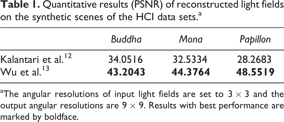
^aThe angular resolutions of input light fields are set to 3 × 3 and the output angular resolutions are 9 × 9. Results with best performance are marked by boldface.

Figure 3.

Comparison of synthetic views produced by Kalentari et al.’s approach¹² and Wu et al.’s approach¹³ on synthetic scenes. The results show the ground truth images, error map of the synthetic results in the Y channel, close-up versions of the image portions in the blue and yellow boxes, and the EPIs located at the red line shown in the ground truth view. The EPIs are upsampled to an appropriate scale in the angular domain for better viewing. The lowest image in each block shows a close-up of the portion of the EPIs in the red box.

The numerical results of depth maps using the approaches by Tao et al.²⁴ and Wang et al.²⁵ are tabulated in Table 2. And Figure 4 demonstrates the depth maps estimated by Wang et al.’s approach²⁵ on the Buddha using input low angular resolution (3 × 3) light field, ground truth (GT) high-resolution (9 × 9) light field and super-resolved light fields (9 × 9) by Kalantari et al.¹² and Wu et al.,¹³ respectively. The depth estimation using super-resolved light fields shows prominent improvement when compared with the results using input low-resolution light fields. In addition, due to the better quality of synthetic views produced by Wu et al.’s approach,¹³ especially in the occluded regions, the estimated depth maps are more accurate than those using super-resolved light fields by Kalantari et al.’s approach.¹²

Table 2.

RMSE values of the estimated depth using the approaches by Tao et al.^{24/Wang et al.25} on synthetic scenes of HCI data sets.

	Buddha	Mona	Papillon
Input views	0.2642/0.2926	0.2115/0.2541	0.1871/0.1533
Kalantari et al.¹²	0.1721/0.1576	0.0876/0.0829	0.1665/0.1430
Wu et al.¹³	0.0550/0.0401	0.0678/0.0517	0.0610/0.0532
GT Light Fields	0.0543/0.0393	0.0652/0.0529	0.0583/0.0455

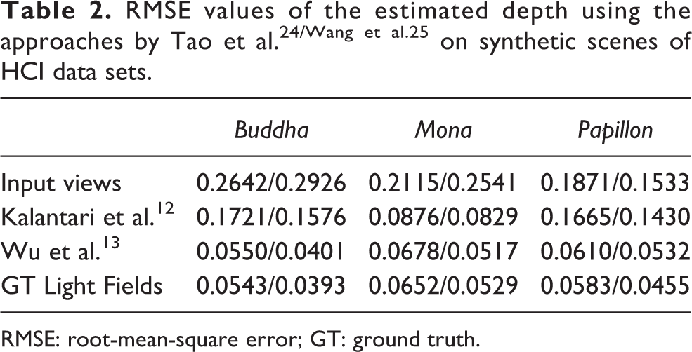
RMSE: root-mean-square error; GT: ground truth.

Figure 4.

Comparison of depth maps estimated by Wang et al.’s approach²⁵ using light fields of different angular resolutions on the Buddha.

Real-world scenes

The Stanford Lytro Light Field Archive²⁷ is used for the evaluation on real-world scenes. The data set is divided into several categories including occlusions, and refractive and reflective surfaces, which are challenge cases to test the robustness of the approaches. We use 3 × 3 views to reconstruct 7 × 7 light fields.

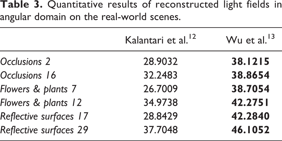
Table 3 lists the numerical results of the super-resolution approaches on the real-world scenes. The approach by Wu et al.¹³ shows better performance in terms of PSNR. Figure 5 shows some representative cases that contain complex occlusions or darkened scene. The networks proposed by Kalantari et al.¹² were specifically trained for Lambertian regions, and thus tend to fail in the reflective surfaces, such as lamplight in the Plants 12 case. In addition, due to the depth estimation-based framework, the synthetic views have ghosting and tearing artifacts in the occlusion boundaries, such as the red flower in the IMG 1328 case and the twig located in yellow box in the Flowers 6 case. The error map also reflects the reconstruct method performance, especially in some special regions.

Table 3.

Quantitative results of reconstructed light fields in angular domain on the real-world scenes.

	Kalantari et al.¹²	Wu et al.¹³
Occlusions 2	28.9032	38.1215
Occlusions 16	32.2483	38.8654
Flowers & plants 7	26.7009	38.7054
Flowers & plants 12	34.9738	42.2751
Reflective surfaces 17	28.8429	42.2840
Reflective surfaces 29	37.7048	46.1052

Figure 5.

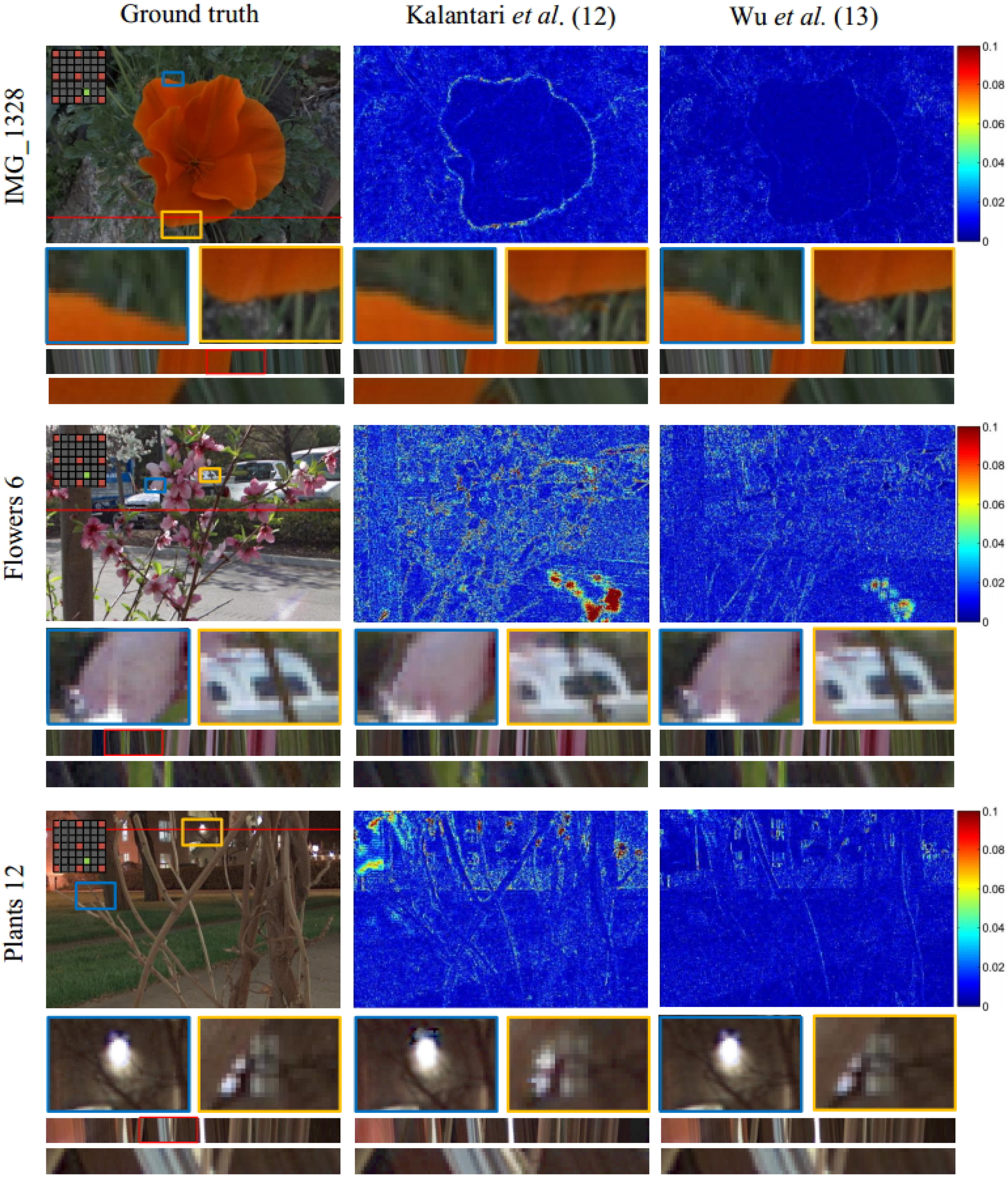
Comparison of synthetic views produced by Kalentari et al.’s approach¹² and Wu et al.’s approach¹³ on real-world scenes. The results show the ground truth images, error maps of the synthetic results in the Y channel, close-up versions of the image portions in the blue and yellow boxes, and the EPIs located at the red line shown in the ground view. The EPIs are upsampled to an appropriate scale in the angular domain for better viewing. The lowest image in each block shows a close-up of the portion of the EPIs in the red box.

Figure 6 shows the depth maps estimated by Tao et al.’s approach²⁴ and Wang et al.’s approach²⁵ using input low angular resolution (3 × 3) light field, super-resolved light fields (7 × 7) by Wu et al.,¹³ and ground truth high-resolution (7 × 7) light field. The quality of estimated depth maps are significantly improved using super-resolved light fields.

Figure 6.

Comparison of depth maps estimated by Tao et al.²⁴ and Wang et al.²⁵ using light fields of different angular resolutions on the Reflective surfaces 29.

Spatial super-resolution results

In this section, we mainly evaluate two spatial super-resolution methods as mentioned previously on several data sets including synthetic and real-world scenes. For the light field data sets, we evaluate these methods in the scaling factor of × 4. We keep the central image of the light field unchanged and the rest of the low resolution (LR) source images $I_{s}^{L}$ are obtained by downsampling the high resolution (HR) images which act as the ground truth for computing PSNR value. The HR image located in the center is regarded as the reference image, that is, $I_{r}^{H}$ . We utilize the bicubic interpolation, PaSR, and iPADS methods on the different data sets.

Synthetic scenes

We test the synthetic light field data from the HCI data sets.²⁶ The super-resolution scaling factor is ×4, which evaluates the performance of the proposed framework. The spatial resolution of the original light field image is 768 × 768, and the angular resolution is 9 × 9. The spatial resolution of the input light fields is downsampled by a factor of 4. Through these methods, we super-resolve the spatial resolution for a factor of ×4.

Figure 7 shows several super-resolution patches cropped from the six simulations. Because of the iterative operation, it is obvious that the patches generated by iPADS method contain better high-frequency details than those generated by bicubic interpolation and PaSR method, especially, for patches with large depth variations. Table 4 shows a quantitative evaluation (PSNR) of the super-resolution approaches on synthetic scenes. The results of iPADS method produce the highest quality of all the methods. The bicubic interpolation is a simple upsampling method. We get these results as the reference.

Figure 7.

Comparison of spatial super-resolution results produced by PaSR method¹² and iPADS method¹³ on synthetic scenes.

Table 4.

Quantitative results of reconstructed light fields on the synthetic scenes of the HCI data sets.^a

	Buddha	Papillon	StillLife
Bicubic	29.8126	32.1981	21.9496
PaSR²⁰	32.0326	36.4879	25.4685
iPADS²¹	33.7775	38.4358	25.8911

PaSR: PatchMatch-based super-resolution; iPADS: Patch- And Depth-based Synthesis.

^aThe spatial super-resolutions scaling factor is ×4.

Table 5 shows the numerical results of depth maps. We calculate RMSE value with the ground truth depth map. We can conclude that the smaller the value is, the more accurate will be the depth map. The spatial super-resolution method does improve the accuracy of estimated depth map, when comparing with the method of bicubic upsampling. Figure 8 provides a further verification. The noisy point in the background decreases as the RMSE value goes down.

Table 5.

RMSE values of the estimated depth using the approaches by Wang et al.²⁵ on synthetic scenes of HCI data sets.

	Buddha	Papillon	StillLife
Bicubic	0.3186	0.2039	0.3718
PaSR²⁰	0.2968	0.1549	0.3049
iPADS²¹	0.2021	0.0685	0.2902
GT Light Fields	0.0854	0.0490	0.0998

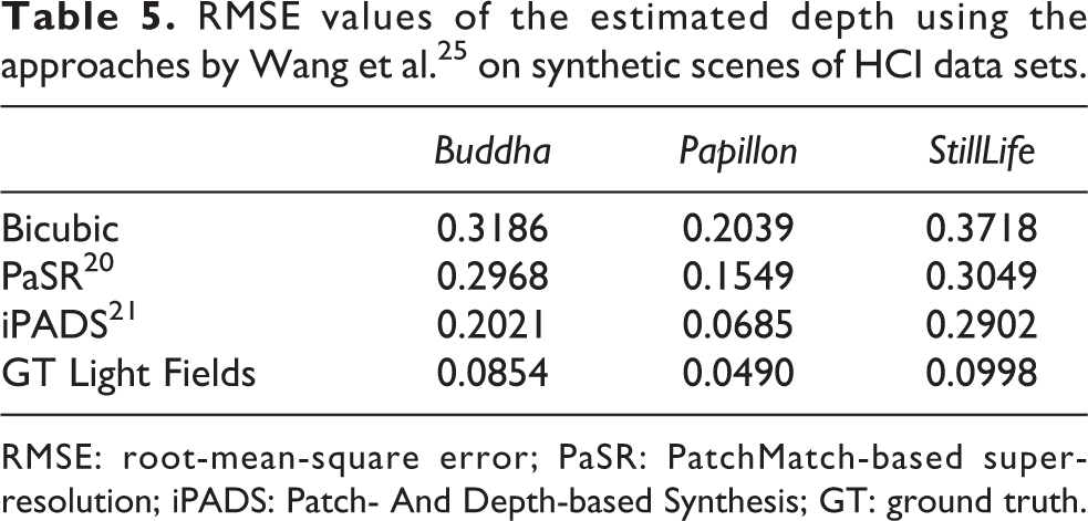
RMSE: root-mean-square error; PaSR: PatchMatch-based super-resolution; iPADS: Patch- And Depth-based Synthesis; GT: ground truth.

Figure 8.

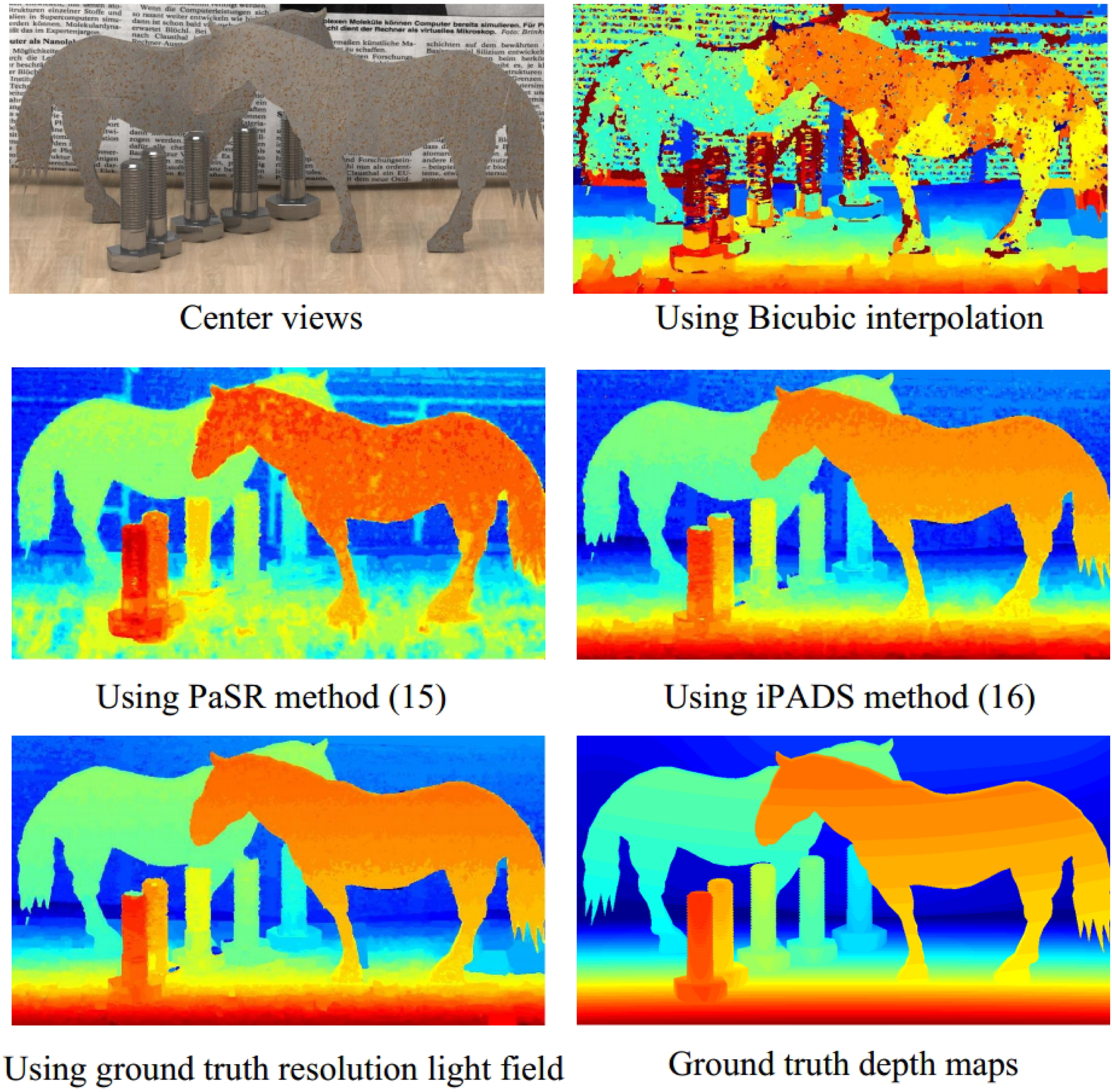
Comparison of depth maps estimated by Wang et al.’s approach²⁵ using light fields of different spatial resolutions on the Horses. Spatial super-resolution results produced by PaSR method¹² and iPADS method¹³ on synthetic scenes. The spatial super-resolutions scaling factor is ×4. PaSR: PatchMatch-based super-resolution; iPADS: iterative Patch- And Depth-based Synthesis.

Real-world scenes

The Stanford Lytro Light Field Archive²⁷ is also used for the evaluation on real-world scenes. We first downsample the light field by a factor of 4 in the spatial domain, and then utilize the mentioned PaSR method to reconstruct the light field. Table 6 lists the numerical results of the super-resolution methods on the real-world scenes. Each PSNR value is obtained by averaging over the PSNRs of all side views. The PSNR values are obtained using both iPADS and PaSR method. The PSNRs for iPADS method are higher than those for PaSR method in each data set. The direct interpolation method, such as bicubic interpolation, has the lowest values among all the methods.

Table 6.

Quantitative results of reconstructed light fields in spatial domain on the real-world scenes.

	Bicubic	PaSR¹¹	iPADS¹²
Occlusions 2	25.9651	31.4563	32.0949
Occlusions 16	26.0196	30.9683	31.7601
Flowers & plants 7	26.3130	30.6409	32.0742
Flowers & plants 12	27.5439	31.0064	33.0185
Reflective surfaces 17	27.0124	32.7958	33.1532
Reflective surfaces 29	27.4583	30.2019	32.9482

PaSR: PatchMatch-based super-resolution; iPADS: Patch- And Depth-based Synthesis.

Figure 9 shows some representative cases.²⁷ The Flower 3 scene contains complex occlusions, and the Reflective 29 scene contains metallic pans, which have non-Lambertian surfaces. The results of bicubic interpolation have serious blur and the iPADS method can restore the high-frequency details.

Figure 9.

Comparison of spatial super-resolution results produced by bicubic interpolation, PaSR method,¹² and iPADS method¹³ on real-world scenes. PaSR: PatchMatch-based super-resolution; iPADS: iterative Patch- And Depth-based Synthesis.

For a more intuitive understanding of what Table 6 means, we provide the depth estimation results of the case, Reflective 29, as shown in Figure 10. The figure shows the depth maps estimated by Wang et al.’s approach²⁵ using input bicubic directly interpolation light field, super-resolved light fields by iPADS method²¹ and ground truth original resolution light field, respectively. The quality of estimated depth maps is also significantly improved using super-resolved light fields.

Figure 10.

Comparison of depth maps estimated by Wang et al.²⁵ using light fields of different spatial resolutions on the Reflective surfaces 29.

Spatio-angular super-resolution results

In this section, we super-resolved the light field both in angular and spatial domains, simultaneously. We hope that we can get a better depth estimation result. Because the spatial super-resolution algorithm can tolerate the larger parallax, usually reach up to 15 pixels in the reference image level, we first carry on super-resolution in the spatial domain. Once we obtain the super-resolved spatial light field, we synthesize angular views through reconstructed high-resolution spatial images.

We utilize the MonasRoom from HCI data set as an example, the input light field of the whole precess is 3 × 3 views in the angular resolution, and 192 × 192 pixels in the spatial resolution. The output is 9 × 9 views in the angular resolution and 768 × 768 pixels in the spatial resolution. The pipleline of spatio-angular super-resolution is shown in Figure 11. To obtain the final spatio-angular super-resolution result (as shown in Figure 11 (d)), we first handle it in spatial domain (Figure 11 (c)), and then take super-resolution in angular domain (Figure 11 (b)).

Figure 11.

The pipeline of the spatio-angular super-resolution process. (a) is the input light field with sparse view in angular domain and low-resolution in spatial domain. (c) is the super-resolved light field in spatial domain. And then we carry on super-resolution in angular domain (b) to obtain the final spatio-angular super-resolution result (d).

Figure 12 shows the depth maps estimated by Wang et al.²⁵ The input light field has different resolutions. The subfigures (a), (b), (c), and (d) of Figure 12 are depth maps, and their inputs are Figure 11 (a), (b), (c) and (d), respectively. We notice that the depth map using spatio-angular super-resolution result (Figure 12 (d)) is similar to the depth map using ground truth light field. What’s more, the depth map using spatio-angular super-resolution result should be very close to the ground truth depth map. So our strategy of estimating depth map is very advisable. Table 7 further proves the effectiveness of this strategy, and the super-resolution of the light field can indeed improve the accuracy of the depth map significantly.

Figure 12.

Comparison of depth maps estimated by Wang et al.²⁵ using light fields of different resolutions on the Monas Room.

Table 7.

RMSE values of the estimated depth using LR light field, SR result in the angular domain, SR in the spatial domain, and GT light field.

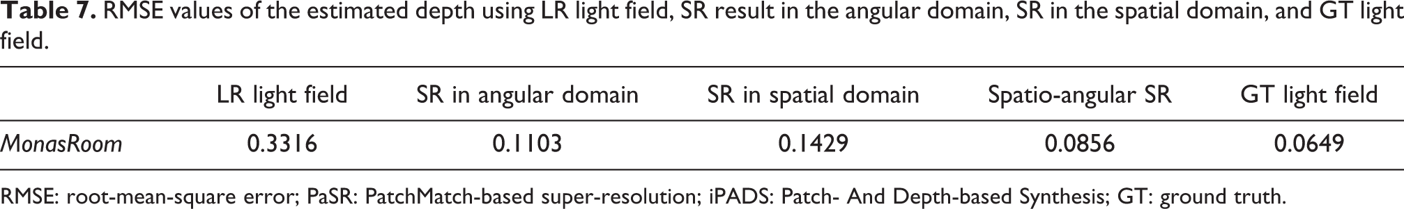
	LR light field	SR in angular domain	SR in spatial domain	Spatio-angular SR	GT light field
MonasRoom	0.3316	0.1103	0.1429	0.0856	0.0649

RMSE: root-mean-square error; PaSR: PatchMatch-based super-resolution; iPADS: Patch- And Depth-based Synthesis; GT: ground truth.

Conclusions

We have presented an idea that uses an super-resolved light field (including angular and spatial domains) to improve the quality of depth estimation. A straightforward way is to estimate a depth map using input low-resolution light field, and render novel views or interpolate images in spatial domain using depth image based rendering (DIBR) techniques. However, this approach always leads to error accumulation when we recompute depth maps. We therefore investigate approaches that directly minimize the quality of super-resolved light fields rather than depth maps. We evaluate this idea on synthetic scenes as well as real-world scenes which contain non-Lambertian and reflective surfaces. The experimental results demonstrate that the quality of depth map is significantly improved using the super-resolved light field.

Footnotes

Authors’ note

This article was presented in part at the CCF Chinese Conference on Computer Vision, Tianjin, 2017. This article was recommended by the program committee.

Declaration of conflicting interests

The author(s) declared no potential conflicts of interest with respect to the research, authorship, and/or publication of this article.

Funding

The author(s) disclosed receipt of the following financial support for the research, authorship, and/or publication of this article: This work was supported by the National Key Foundation for Exploring Scientific Instrument (Grant No. 2013YQ140517) and the NSF of China (Grant Nos. 61522111 and 61531014).

References

Levoy

Hanrahan

. Light field rendering. In: Proceedings of the 23rd annual conference on Computer graphics and interactive techniques. ACM, 1996, pp. 31–42.

Ihrke

Restrepo

Mignard-Debise

. Principles of light field imaging: briefly revisiting 25 years of research. IEEE Signal Process Mag 2016; 33(5): 59–69.

Lippmann

. Epreuves reversibles donnant la sensation du relief. J Phys Theor Appl 1908; 7(1): 821–825.

Lytro, 2017. [Online]. Available: https://www.lytro.com/.

RayTrix. 3D light field camera technology, 2017. [Online]. Available: http://www.raytrix.de/.

Pujades

Devernay

Goldluecke

. Bayesian view synthesis and image-based rendering principles. In: CVPR. IEEE, 2014, pp. 3906–3913.

Shi

Hassanieh

Davis

. Light field reconstruction using sparsity in the continuous fourier domain. ACM TOG 2014; 34(1): 12.

Vagharshakyan

Bregovic

Gotchev

. Image based rendering technique via sparse representation in shearlet domain. In: ICIP. IEEE, 2015, pp. 1379–1383.

Yoon

Jeon

Yoo

. Learning a deep convolutional network for light-field image super-resolution. In: ICCV Workshops. IEEE, 2015, pp. 24–32.

10.

Zhang

Liu

Dai

. Light field from micro-baseline image pair. In: CVPR. IEEE, 2015, pp. 3800–3809.

11.

Wanner

Goldluecke

. Variational light field analysis for disparity estimation and super-resolution. IEEE TPAMI 2014; 36(3): 606–619.

12.

Kalantari

Wang

Ramamoorthi

. Learning-based view synthesis for light field cameras. ACM Trans Graph (TOG) 2016; 35(6): 193.

13.

Zhao

Wang

. Light field reconstruction using deep convolutional network on EPI. In: CVPR. IEEE, 2017, pp. 12–21.

14.

Stanford (New) Light Field Archive, 2008. [Online]. Available: http://lightfield.stanford.edu/lfs.html.

15.

Eigen

Puhrsch

Fergus

. Depth map prediction from a single image using a multi-scale deep network. In: Advances in Neural Information Processing Systems, NIPS, 2014, pp. 2366–2374.

16.

Krizhevsky

Sutskever

Hinton

. Imagenet classification with deep convolutional neural networks. In: Advances in Neural Information Processing Systems, NIPS, 2012, pp. 1097–1105.

17.

Dong

Loy

. Learning a deep convolutional network for image super-resolution. In: ECCV. Springer, 2014, pp. 184–199.

18.

Jia

Shelhamer

Donahue

. Caffe: convolutional architecture for fast feature embedding. In: ACM MM. ACM, 2014, pp. 675–678.

19.

Zhao

Liu

. How depth estimation in light fields can benefit from angular super-resolution? In: CCCV. Springer, Singapore, 2017, pp. 12–21.

20.

Boominathan

Mitra

Veeraraghavan

. Improving resolution and depth-of-field of light field cameras using a hybrid imaging system. In: ICCP. IEEE, 2014, pp. 1–10.

21.

Wang

Liu

Heidrich

. The light field attachment: turning a DSLR into a light field camera using a low budget camera ring. IEEE Trans Visual Comput Graph (TVCG) 2016; 23(10): 2357–2364.

22.

Bishop

Zanetti

Favaro

. Light field superresolution. In: IEEE international conference on Computational photography (ICCP-2009). IEEE, pp. 1–9.

23.

Zhang

Wang

Shechtman

. Plenopatch: patch-based plenoptic image manipulation. IEEE TVCG 2017; 23(5): 1561–1573.

24.

Tao

Hadap

Malik

. Depth from combining defocus and correspondence using light-field cameras. In: ICCV. IEEE, 2013, pp. 673–680.

25.

Wang

Efros

Ramamoorthi

. Occlusion-aware depth estimation using light-field cameras. In: ICCV. IEEE, 2015, pp. 3487–3495.

26.

Wanner

Meister

Goldlücke

. Datasets and benchmarks for densely sampled 4d light fields. In: Vision, Modeling & Visualization, Citeseer, 2013, pp. 225–226.

27.

Stanford Lytro Light Field Archive, 2017. Available at: http://lightfields.stanford.edu/.

How depth estimation in light fields can benefit from super-resolution?

Abstract

Keywords

Introduction

Depth estimation using super-resolved light fields

Angular super-resolution for light fields

CNN architecture

Training detail

Spatial super-resolution for light fields

Depth estimation for light fields

Experimental results

Angular super-resolution results

Synthetic scenes

Real-world scenes

Spatial super-resolution results

Synthetic scenes

Real-world scenes

Spatio-angular super-resolution results

Conclusions

Footnotes

Authors’ note

Declaration of conflicting interests

Funding

References