Sage Journals: Discover world-class research

Abstract

This article proposes a novel approach for the two-wheel-steer four-wheel-drive vehicle path tracking based on force control. Both the kinematic and dynamic models are used to calculate the virtual inputs based on a model predictive control algorithm. By using these virtual inputs as the constraints of a real-time sequential quadratic programming optimization, the optimal real inputs such as the drive forces and the steering angles are obtained. Note that the system is discretized when designing the control algorithm. The novelty is that all the forces are taken into account in the dynamic model, and the controller uses optimal steering angles and drive forces to obtain the minimum path offset. The integrated algorithms are then used in tracking a predefined path. Simulation results are provided to demonstrate the effectiveness and applicability of the proposed approach.

Keywords

Ground vehicle force control path tracking model predictive control sequential quadratic programming

Introduction

This article addresses the problem of path tracking applicable to field vehicles. While there are a number of successfully developed path tracking algorithms currently in operation as well as presented in the literature, the demand on extremely high precision path tracking at moderately high speeds is ever increasing. In order to realize better path tracking capabilities, it is of paramount importance to deal with the disturbances that affect the ability to track a path accurately. Among the disturbances are gravitational forces that act on the vehicle when it travels along terrain that slopes towards a side; the inability of the ground to provide the necessary reactionary forces to hold the vehicle on the path, for example, due to sandy or soft soil; and in some cases such as construction, mining and agriculture, the forces due to the machine engaging the ground.

In order to design sound control algorithms, it is essential to develop system models that accurately represent the ground vehicle being modeled. The two primary modeling methods used, namely, the kinematic models and the dynamic models have their own advantages and disadvantages. A kinematic model is developed by ignoring the inertial effects and on the assumption that velocities can be used as inputs. On the contrary, a dynamic model is developed by taking into account all the inertial effects and considering forces as the inputs. Undoubtedly, a dynamic model is an accurate representation of what goes on in real life provided the modeling can be done accurately.

In the current research, the vehicle path tracking is mainly based on the kinematic models due to their simplicity. Kinematic-based control algorithms are developed using offset model derived from the vehicle kinematic model. Normally, the kinematic model is approximated by the bicycle model or the tricycle model in which the steering angle of the front wheel is used to orientate the vehicle.^1
–3 In order to improve the robustness and reliability of the controller, the slip effects are incorporated in the kinematic modeling. Among the many controller design method available are sliding mode control (SMC), back-stepping control (BSC), and model predictive control (MPC). Zhou et al.⁴ proposed a new robust SMC method which is implemented by considering the dynamic characteristics of the vehicle. A more elaborate way to deal with wheel slip was presented by Taghia and Katupitiya,⁵ in which the authors dealt with the slip through the use of a slip observer, then an SMC is used to achieve a successful path tracking control. In the research of Fang et al.⁶ a BSC based controller is designed which considers the slip effects as additive unknown parameters to the ideal kinematic model. Lenain et al.⁷ proposed an MPC algorithm to control the vehicle’s path following while the vehicle is subjected to sliding, and in its follow-up study,⁸ a slip estimator is used in an MPC in combination with a Kalman filter which led to keeping the tracking error within ±15 cm.

These researches have shown that the controllers designed based on kinematic models perform just as good as the controllers designed based on dynamic models provided the operating conditions do not make the dynamical effects dominant. However, it can be seen that an obvious difficulty in kinematic model-based control algorithms is the incorporation of wheel slip, which is primarily due to the difficulties in measuring them. Thus, this assumption is valid only for ground vehicles operating on rather undisturbed ground at low speeds, in which situation the slip forces and slip velocities are not considerable and can be treated as disturbances. For the situations where the vehicles are expected to operate at higher speed or on slippery ground, it is essential to use a dynamic model.^9,10 Regardless of the type of model used, the disturbances that are affecting the motion of the vehicle must be incorporated and taken into account in the model.¹¹ Thus, a more direct way of taking the slip effects into account is to use a dynamic model in which the slip effects can be incorporated as slip forces where the slip forces are either measurable or can be estimated.

In recent years, more researches on dynamic model-based path tracking implementation have been presented.^12
–14 The controllability of the vehicles can be significantly improved by allowing more freedom in the control efforts. In two-wheel-steer four-wheel-drive (2WS4WD) vehicles, this can be achieved by allowing the independent control of all drive forces and steering angles. The 2WS4WD system is an overactuated system and one way of obtaining a solution is to use robust control algorithm in combination with optimization that can be implemented in real time. Yang et al.¹⁵ proposed a hybrid optimal fault-tolerant control approach which combines the linear-quadratic control method, and the Lyapunov method is proposed for a path tracking system. The dynamic model is developed and applied in an objective function, which is optimized by a particle swarm optimization (PSO) algorithm to obtain the optimal drive and steering motions for tracking the planned path precisely.¹⁶ To analyze the effect of the optimization method, the genetic algorithm and the PSO algorithm are compared in real-time path tracking.¹⁷ Among all the optimization methods available, the sequential quadratic programming (SQP) can be effectively used to solve the nonlinear constrained problems, which is the type of optimization associated with the dynamic model-based path tracking implementation.^18,19

In this article, we will be using a complete dynamic model in x, y, and θ space, taking into account all the forces exerted on the vehicle by the ground and all inertial forces.²⁰ Given that the vehicle presented in this study is a four-wheeled vehicle, with the ability to independently steer two of the steered wheels and with the ability to independently drive all four wheels, the significant external forces acting on the vehicle occur at the wheels. The forces at the wheels can be categorized into two different varieties: the longitudinal forces and the lateral forces. If a wheel is driven, the longitudinal force becomes a resultant drive force, and if the vehicle is idling, the longitudinal force becomes a rolling resistance. The lateral forces on the other hand are the forces that hold the vehicle on its intended path. When the lateral forces are insufficient, the vehicle drifts off course. In path tracking, the requirement therefore is to ensure sufficient lateral forces are generated so that the vehicle is kept on its path at all times.

As mentioned before, the vehicle being controlled has four drive forces and two steering angles to be controlled. This also means that there is no link such as the tie rod coupling the steering angles of the two wheels being steered. As such, the steering of the two wheels can be independently controlled. The wheels can also be driven completely independently and therefore requires four drive forces. In total, there are six control inputs. The configuration of six inputs can significantly improve the vehicle’s performance in overcoming the complex disturbances compared to the kinematic model-based vehicles. However, it also leads to an overactuated system problem.

Thus, as the contribution in this work, an integrated MPC algorithm that combines a solution obtained using MPC method applied to a kinematic model and a solution obtained using MPC applied to a dynamic model is presented. These results are further combined in an optimization algorithm to obtain the real inputs such as the drive forces and the steering angles. The MPC applied to the kinematic model provides a set of constraints used in the optimization. The MPC applied to the dynamic model provides a set of virtual accelerations that will also be used as further constraints. Given that the system is an overactuated system, a new objective function is proposed and an SQP-based optimization method is used to solve the control allocation issue.

The article is organized as follows. “Vehicle system modeling” section describes the models needed by the controller, including the vehicle kinematic model, dynamic model, offset model, and wheel model. “Control algorithm and its implementation” section presents the control algorithm, including the integrated MPC algorithm and the SQP optimization method. In “Results and discussion” section, the simulation results are discussed in detail and compared with different control algorithms. Finally, this article is concluded in the last section.

Vehicle system modeling

This section presents the model of the vehicle system, which consists of three submodels: kinematic model, dynamic model, and wheel model. The kinematic model considers the vehicle’s steering angle and velocities, while the dynamic model is subjected to the contact forces generated by the ground. Based on the kinematic and dynamic models, two offset models are proposed for the path tracking problem. As a part of the dynamic model, the wheel model presented in the end describes the actual forces acting on each wheel.

Vehicle kinematic model

Model description

As shown in Figure 1, the vehicle kinematic model is considered as a bicycle model in that the steered wheels at the front are represented with a single wheel at point C and the rear wheels are represented by a single wheel at point D. The length of the vehicle is illustrated in the figure where the front length L_f and the rear length L_r are measured with respect to the center of gravity G. In this model, V_l and V_r are the longitudinal velocity and lateral velocity of the vehicle at point G, respectively. Considering the 2WS4WD vehicle, in its kinematic model, the front wheel is steerable and the steering angle is presented as δ, while the rear wheel is nonsteerable. O_t is defined as the instantaneous center of rotation of the vehicle. V_fw and V_rw are the resultant velocities of the front wheel and the rear wheel, respectively. α_f represents the slip angle of the front wheel. The positive direction of both the steering angle and slip angle is set to be clockwise.

Figure 1.

Kinematic model and its offset model.

In order to facilitate the description of the vehicle kinematic states, a state vector q_k is defined as $q_{k} = [x_{k}, y_{k}, θ_{k}]$ , in which (x_k , y_k ) is the position of center of gravity G in the global coordinate frame, while θ_k is the orientation of the vehicle longitudinal axis. Note that all variables are defined in continuous-time domain and the subscript k implies the kinematic model. Referring to Huynh et al.,²¹ the kinematic equations are expressed as

\begin{matrix} {\dot{x}}_{k} = V_{l} cos θ_{k} - V_{r} sin θ_{k} \\ {\dot{y}}_{k} = V_{l} sin θ_{k} + V_{r} cos θ_{k} \\ {\dot{θ}}_{k} = \frac{V_{l}}{L_{f}} tan (δ - α_{f}) + \frac{V_{r}}{L_{f}} \end{matrix}

Kinematic model-based offset model

In order to develop the kinematic model-based controller, the kinematic model-based offset model (KBOM) must be developed. As shown in Figure 1, l_os denotes the offset error between the center of gravity G and the closest point on the reference path, while θ_os denotes the heading error. Particularly, we have |l_os | = |GP| and θ_os = θ_k − θ_d , where point P is the reference point and θ_d is the desired orientation at P. Point P can be obtained by comparing the distances from CG to all the point on reference path.²² For the path tracking system, the KBOM can describe the relationship between errors and velocities, which is written as

\begin{matrix} {\dot{l}}_{o s} = V_{l} \cdot sin θ_{o s} + V_{r} \cdot cos θ_{o s} - V_{r d} \\ {\dot{θ}}_{o s} = \frac{V_{l}}{L_{f}} tan (δ - α_{f}) + \frac{V_{r}}{L_{f}} - ω_{d} \end{matrix}

where V_rd and ω_d are the desired lateral velocity and angular velocity at reference point P, respectively.

To be applied in the MPC algorithm, the KBOM needs to be linearized. In this offset model, for a controlled vehicle, we define that the heading error θ_os should satisfy a range [−10°, 10°], and we define V_r ⋅ cosθ_os ≈ V_r . This assumption is valid when the vehicle is controlled by the dynamic controller. Moreover, as the second assumption, the amount of slip at the wheels α_f can be ignored and the desired lateral velocity V_rd is set to be zero at this stage. Because at this stage, the kinematic model is used as a virtual model of the vehicle. Later in the dynamic modeling, the slip forces are incorporated to make the vehicle model more realistic. Based on the above assumptions, the KBOM in equation (2) can be simplified as

\begin{matrix} {\dot{l}}_{o s} = V_{l} \cdot sin θ_{o s} + V_{r} \\ {\dot{θ}}_{o s} = \frac{V_{l}}{L_{f}} tan (δ) + \frac{V_{r}}{L_{f}} - ω_{d} \end{matrix}

From the simplified KBOM, the state variables, x ₁ and x ₂, and the new input u are defined as follows

\begin{matrix} x_{1} = l_{o s} \\ x_{2} = V_{l} \cdot sin θ_{o s} + V_{r} \\ u = V_{l} \cdot cos θ_{o s} (\frac{V_{l}}{L_{f}} tan (δ) + \frac{V_{r}}{L_{f}} - ω_{d}) \end{matrix}

Then, the model can be rewritten as

\begin{matrix} {\dot{x}}_{1} = x_{2} \\ {\dot{x}}_{2} = u_{k} + d \end{matrix}

where

\begin{array}{l} d = {\dot{V}}_{r} . \end{array}

In this model, the derivative of the lateral velocity V_r is considered as the measured disturbance within a small range. In the application of control algorithm, the value of d can be obtained relying on the feedback from the global position system (GPS) directly.

According to the control objective of the model, we define the state vector and output vector as X_k = [x ₁ x ₂]^T and Y_k = [x ₁ x ₂]^T, respectively. Then, the model can be obtained as a standard linear state space model ${\dot{X}}_{k} = A_{k} X_{k} + B_{k} u_{k}$ and Y_k = C_kX_k , where $A_{k} = [\begin{matrix} 1 & 0 \\ 0 & 0 \end{matrix}]$ , $B_{k} = [\begin{matrix} 0 \\ 1 \end{matrix}]$ , and $C_{k} = [\begin{matrix} 1 & 0 \\ 0 & 1 \end{matrix}]$ .

Vehicle dynamic model

In this section, the vehicle dynamic model and the offset model for force control are presented.

Model description

The vehicle dynamic modeling is illustrated in Figure 2. The 2WS4WD vehicle body is considered as a rigid body which has a constant mass M and inertia J. The vehicle is driven by four wheels, in which the front wheels are steerable while the rear wheels are nonsteerable. To simplify the derivations, the dynamic analysis is made at the center of gravity. θ is the orientation of the vehicle, and a_x , a_y , and γ represent the accelerations in x-direction, y-direction, and angular acceleration of the vehicle about a vertical axis, respectively. V_l and V_r represent the longitudinal and lateral velocity in the local coordinate frame, while a_l and a_r represent the longitudinal and lateral acceleration in the local coordinate frame. 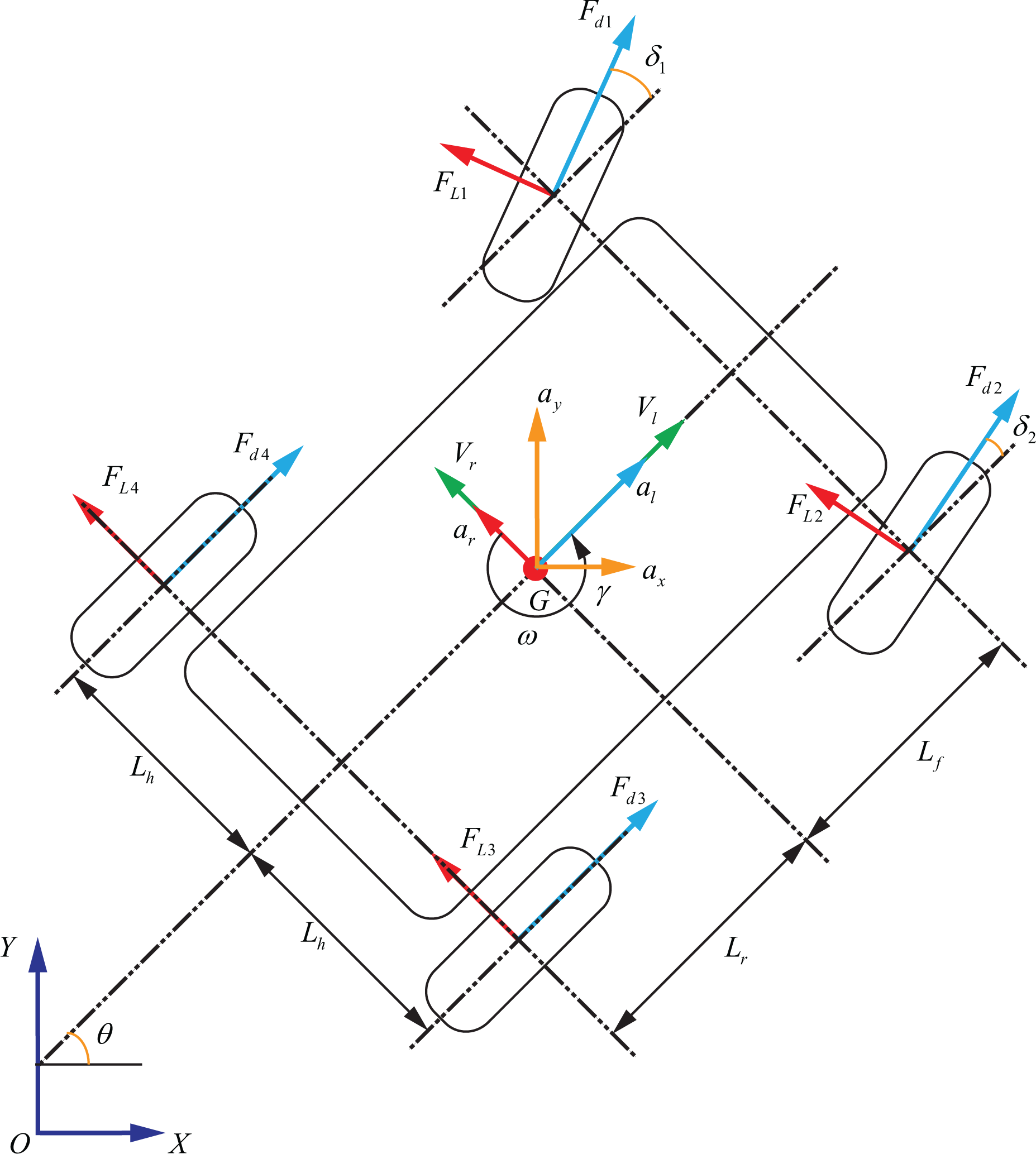$F_{d i} (i = 1, ..., 4)$ and $F_{L i} (i = 1, ..., 4)$ are the longitudinal forces and lateral forces at wheels, respectively. The two steering angles of each wheel are $δ_{i} (i = 1, ..., 4)$ .

Figure 2.

Dynamic model of the vehicle.

The dynamic equations of the 2WS4WD vehicle are written as

\begin{matrix} M a_{x} = \sum_{i = 1}^{4} (F_{d i} \cdot cos (θ + δ_{i}) - F_{L i} \cdot sin (θ + δ_{i})) \\ M a_{y} = \sum_{i = 1}^{4} (F_{d i} \cdot sin (θ + δ_{i}) + F_{L i} \cdot cos (θ + δ_{i})) \\ J γ = \sum_{i = 1}^{4} [L_{y i} \cdot (- F_{d i} \cdot cos δ_{i} + F_{L i} \cdot sin δ_{i}) \\ + L_{x i} \cdot (F_{d i} \cdot sin δ_{i} + F_{L i} \cdot cos δ_{i})] \end{matrix}

where $(L_{x i}, L_{y i})$ represents the location of each wheel in a coordinate system with its origin at center of gravity and positive x-axis forward. Note that in 2WS4WD vehicle, only two front wheels are steerable and the steering angles δ ₃ and δ ₄ are always zero in the model.

Offset model for the force control

In this work, we proposed an offset model specific to the ground vehicle force control which is named as offset model for the force control (OMFC) in this article. To analyze the error of the path tracking system more accurately, not only the offset error and the heading error but also their velocity errors and acceleration errors need to be considered. Thus, the OMFC is presented as shown in Figure 3.

Figure 3.

Offset model for the force control.

In this model, the reference point is still set as point P which means l_os and θ_os have the same definition of that in KBOM. Thus, the desired velocities V_ld , V_rd , and ω_d and accelerations A_ld , A_rd , and γ_d can be obtained directly from the reference path properties when P is targeted.

To begin with constructing this model, the derivative of l_os will firstly be considered. It is obvious that ${\dot{l}}_{o s}$ is the rate of change of |GP| which is subjected to the decomposed velocities in its direction. Hence, the first equation is written as

{\dot{l}}_{o s} = V_{l} \cdot sin θ_{o s} + V_{r} \cdot cos θ_{o s} - V_{r d}

The second derivative of l_os can be derived by taking time derivative of equation (7). Thus, the equation about ${\ddot{l}}_{o s}$ is written as

\begin{matrix} {\ddot{l}}_{o s} = A_{l} \cdot sin θ_{o s} + A_{r} \cdot cos θ_{o s} - A_{r d} \\ + {\dot{θ}}_{o s} (V_{l} \cdot cos θ_{o s} - V_{r} \cdot sin θ_{o s}) \end{matrix}

Secondly, according to the definition of heading error θ_os , its derivative ${\dot{θ}}_{o s}$ and second derivative ${\ddot{θ}}_{o s}$ are the relative angular velocity and acceleration subjected to reference point, which can be presented as

\begin{array}{l} {\dot{θ}}_{o s} = ω - ω_{d} \\ {\ddot{θ}}_{o s} = γ - γ_{d} \end{array}

In the force control path tracking system, the longitudinal velocity is also considered as a controllable variable subjected to the longitudinal acceleration. Thus, a longitudinal velocity error V_los is defined which denotes the error between the actual longitudinal velocity and the desired longitudinal velocity obtained from the reference path. Hence, the equation of V_los and its derivative are written as

\begin{matrix} V_{l o s} = V_{l} - V_{l d} \\ {\dot{V}}_{l o s} = A_{l} - A_{l d} \end{matrix}

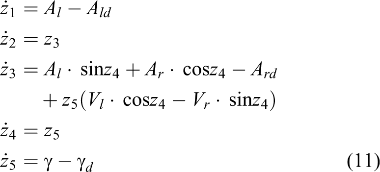
To be applied in the MPC algorithm, the OMFC should be written in state equation form. We define state vector $Z_{f} = [z_{1} z_{2} z_{3} z_{4} z_{5}]^{T}$ , where z ₁ represents the longitudinal velocity of the vehicle, z ₂ and z ₃ represent the offset error and its rate of change, respectively and z ₄ and z ₅ represent the heading error and its rate of change, respectively. By substituting model equations (7) to (10), the state equations can be written as

{\dot{z}}_{1} = A_{l} - A_{l d} {\dot{z}}_{2} = z_{3} {\dot{z}}_{3} = A_{l} \cdot sin z_{4} + A_{r} \cdot cos z_{4} - A_{r d} + z_{5} (V_{l} \cdot cos z_{4} - V_{r} \cdot sin z_{4}) {\dot{z}}_{4} = z_{5} {\dot{z}}_{5} = γ - γ_{d}

It is obvious that this model is nonlinear, where ${\dot{z}}_{3}$ has a trigonometric relationship with z ₄ and z ₅, while the reference accelerations A_ld , A_rd , and γ_d are considered as the measured disturbances in the model. Thus, linearization method for this model is proposed based on the idea of feedback linearization. Since the heading error and its derivative are changing smoothly and can feedback from the state variables, the reference accelerations can be obtained from the reference path properties. We define a virtual input vector $V_{f} = [v_{1} v_{2} v_{3}]^{T}$ to replace the nonlinear part in the model

v_{1} = A_{l} - A_{l d} v_{2} = A_{l} \cdot sin θ_{o s} + A_{r} \cdot cos θ_{o s} - A_{r d} + {\dot{θ}}_{o s} (V_{l} \cdot cos θ_{o s} - V_{r} \cdot sin θ_{o s}) v_{3} = γ - γ_{d}

where θ_os and ${\dot{θ}}_{o s}$ are equal to the current states of z ₄ and z ₅, respectively. In the OMFC, the outputs can be written in a vector $Y_{f} = [z_{1} z_{2} z_{4}]^{T}$ . Then, by substituting the definitions of Z_f , Y_k , and V_f , the linear model can be obtained as a standard linear state space model ${\dot{Z}}_{f} = A_{f} Z_{f} + B_{f} V_{f}$ and Y_f = C_fZ_f .

Wheel model

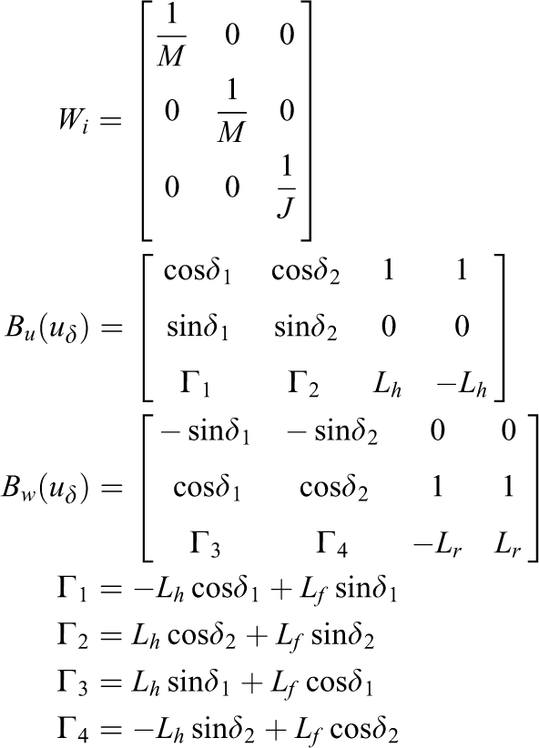
The wheel model is used to describe the drive forces and lateral forces mentioned in the vehicle dynamic model (6). For the drive forces, in this article, we assume that an effective drive unit has been used to generate the drive force needed at each wheel. Based on this assumption, the drive forces F_di are considered as inputs in the force control system. For the lateral forces, according to Woods and Katupitiya,²⁰ it is determined by not only the steering angle but also the actual velocity direction of each wheel. However, the wheel’s actual velocity direction is not a directly controllable variable. Thus, to obtain the sound simulation of the wheel, the lateral force is described subjected to the wheel kinematic properties as well as dynamic properties in the proposed wheel model.

As shown in Figure 4, the lateral forces F_Li occur perpendicular to the plane of the wheel and are a result of the wheels slipping in the lateral directions. The longitudinal slip forces are the forces that occur in the nominal rolling direction of each wheel. The lateral force has a linear relationship with the slip angle α_i when it is within [−5°, 5°]. The relationship is determined by the load at each wheel F_Ni and a lateral slip friction coefficient k_Li which is expressed as

F_{L i} = {\begin{array}{l} k_{L i} F_{N i} α_{i}, & | α_{i} | \leq 5 \\ 5 F_{N i} α_{i}, & α_{i} > 5 \\ - 5 F_{N i} α_{i}, & α_{i} < - 5 \end{array}

Figure 4.

Wheel model.

where k_Li is the lateral slip friction coefficient of the wheel. F_Ni is the load at each wheel which can be calculated by distributing the vehicle’s weight at each wheel. The equations of F_Ni are written as

\begin{array}{l} F_{N 1, 2} = \frac{M g L_{f}}{2 (L_{f} + L_{r})} \\ F_{N 3, 4} = \frac{M g L_{r}}{2 (L_{f} + L_{r})} \end{array}

As shown in Figure 4, the slip angle $α_{i} (i = 1, 2, 3, 4)$ is determined by the steering angle δ_i and the side slip angle β_i which is written as

α_{i} = β_{i} - δ_{i}

where the side slip angle β_i can be calculated by equation (16) according to the dynamic model shown in Figure 4

\begin{array}{l} β_{1} = {tan}^{- 1} (\frac{V_{r} + ω L_{f}}{V_{l} - ω L_{h}}) \\ β_{2} = {tan}^{- 1} (\frac{V_{r} + ω L_{f}}{V_{l} - ω L_{h}}) \\ β_{3} = {tan}^{- 1} (\frac{V_{r} + ω L_{f}}{V_{l} - ω L_{h}}) \\ β_{4} = {tan}^{- 1} (\frac{V_{r} + ω L_{f}}{V_{l} - ω L_{h}}) \end{array}

Control algorithm and its implementation

This section presents the control algorithms in detail. First, the integrated MPC controller is based on an embedded integrator MPC algorithm. The model predictive controller will deliver the virtual control inputs that will control the vehicle in a stable way. Embedded in the virtual control inputs are the real inputs such as the two steering angles and the four drive forces. Then, an SQP is used to carry out optimal control allocation so that the actual inputs to be applied to the physical system can be found. This is achieved by using the virtual control inputs as constraints in the SQP optimization process. A detailed flowchart depicting how all parts of this approach fit together is given later in this section.

Embedded integrator MPC

The MPC algorithm is commonly used to obtain the outputs by solving an online optimization. It has an extensive applicability and strong reliability in controlling different types of systems such as linear system, time-varying or constrained systems. However, one issue is that the MPC algorithm would lead to a large amount of computation in the controller when calculating the optimal solution. For the linear system, because of the particularity of its model, it is probable to get an offline solution directly. An embedded integrator MPC algorithm is proposed and proved to be effective in controlling the linear system without disturbances.²³

Control design

To enable us to develop this model predictive controller, the two offset models KBOM and OMFC presented earlier are written in their general form as

\begin{matrix} \dot{X} = A_{c} X + B_{c} U_{c} \\ Y_{c} = C_{c} X \end{matrix}

where the models presented are continuous-time models. X represents the state vector matrix. U _c is the virtual input vector. Y _c represents the output matrix which is part of the state vector X and can be obtained directly by multiplying the state vector with the matrix C_c .

To apply the MPC algorithm in the real system, the model in equation (17) needs to be discretized. The discrete-time model is written as

\begin{matrix} X_{d} (k + 1) = A_{d} X_{d} (k) + B_{d} U_{d} (k) \\ Y_{d} (k) = C_{d} X_{d} (k) \end{matrix}

where X_d (k), Y_d (k), and U_d (k) are the state vector, output vector, and virtual input vector, respectively. A_d , B_d , and C_d are the matrices after discretization.

Referring to Wang,²³ an augmented state-space model with an embedded integrator can be obtained by defining $Δ X_{d} (k) = X_{d} (k + 1) - X_{d} (k)$ and $Δ u (k) = U_{d} (k + 1) - U_{d} (k)$

\begin{matrix} [\begin{matrix} Δ X_{d} (k + 1) \\ Y_{d} (k + 1) \end{matrix}] = [\begin{matrix} A_{d} & o_{d}^{T} \\ C_{d} A_{d} & I \end{matrix}] [\begin{matrix} Δ X_{d} (k) \\ Y_{d} (k) \end{matrix}] \\ + [\begin{matrix} B_{d} \\ C_{d} B_{d} \end{matrix}] Δ u (k) \\ Y_{d} (k) = [\begin{matrix} o_{d} & I \end{matrix}] [\begin{matrix} Δ X_{d} (k) \\ Y_{d} (k) \end{matrix}] \end{matrix}

where o_d is a zero matrix and I is the identity matrix with the same dimension of Y_d .

Then, the matrix form of augmented model (19) can be simplified by defining $x (k) = [X_{d} {(k)}^{T} Y_{d} {(k)}^{T}]^{T}$ and written as

\begin{matrix} x (k + 1) = A x (k) + B Δ u (k) \\ y (k) = C x (k) \end{matrix}

where

A = [\begin{matrix} A_{d} & o_{d}^{T} \\ C_{d} A_{d} & I \end{matrix}], B = [\begin{matrix} B_{d} \\ C_{d} B_{d} \end{matrix}], C = [\begin{matrix} o_{d}^{T} & I \end{matrix}]

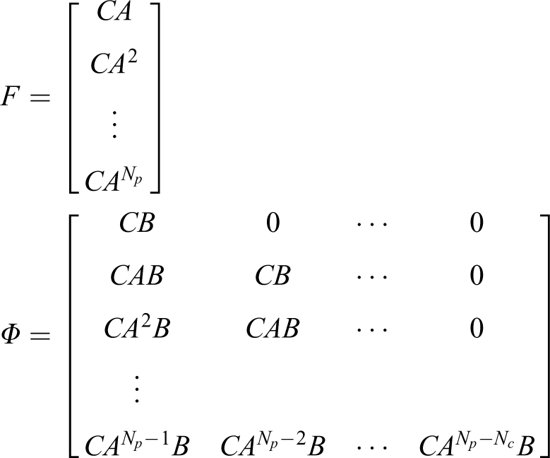
Following the basic idea of MPC, the future outputs can be derived by the linear model proposed earlier. Then, these predictive outputs are compared with the desired outputs. By minimizing the error between the two outputs and the future inputs, the optimal inputs can be obtained. Here, we assume that k_i is the sample time, while y(k_i + n|k_i ) denotes the predictive outputs at time k_i + n based on the states at time k_i . N_c and N_p represent the control horizon and the prediction horizon, respectively. To simplify the derivation, we define the predictive outputs Y and the future inputs ΔU as follow

\begin{array}{l} Y = {[\begin{matrix} y (k_{i} + 1 | k_{i}) & y (k_{i} + 2 | k_{i}) & ... & y (k_{i} + N_{p} | k_{i}) \end{matrix}]}^{T} \\ Δ U = {[\begin{matrix} Δ u (k_{i}) & Δ u (k_{i} + 1) & ... & Δ u (k_{i} + N_{c} - 1) \end{matrix}]}^{T} \end{array}

Thus, the relationship between predictive outputs Y and the future inputs ΔU can be presented by the following equation

\begin{array}{l} Y = F x (k_{i}) + Φ Δ U \end{array}

where

\begin{matrix} F = [\begin{matrix} C A \\ C A^{2} \\ ⋮ \\ C A^{N_{p}} \end{matrix}] \\ Φ = [\begin{matrix} C B & 0 & \dots & 0 \\ C A B & C B & \dots & 0 \\ C A^{2} B & C A B & \dots & 0 \\ ⋮ \\ C A^{N_{p} - 1} B & C A^{N_{p} - 2} B & \dots & C A^{N_{p} - N_{c}} B \end{matrix}] \end{matrix}

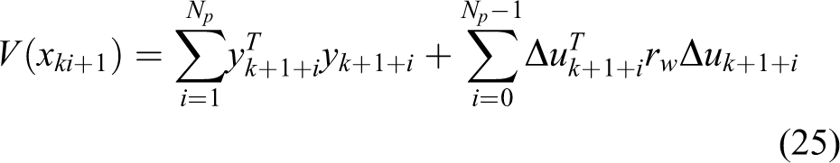
Then the objective function J is defined as

\begin{array}{l} J = (R_{s} - Y)^{T} (R_{s} - Y) + Δ U^{T} \bar{R} Δ U \end{array}

where R_s is the target vector, and $\bar{R}$ is a weighting matrix of ΔU.

By differentiating J and equating it to zero, the optimal solution ΔU* is obtained; however, only the first increment is applied as the control inputs. Thus, the control inputs are Δu(k_i )* and presented as follows

\begin{array}{l} Δ u {(k_{i})}^{*} = \overset{N_{c}}{\overset{︷}{{[1 0 ... 0]}^{T}}} Δ U^{*} = K_{1} - K_{2} x (k_{i}) \end{array}

where

K_{1} = \overset{N_{c}}{\overset{︷}{{[1 0 ... 0]}^{T}}} (Φ^{T} Φ + \bar{R}) - 1 (Φ^{T} R_{s})

K_{2} = \overset{N_{c}}{\overset{︷}{{[1 0 ... 0]}^{T}}} (Φ^{T} Φ + \bar{R}) - 1 (Φ^{T} F)

Finally, the virtual inputs U ^* can be calculated by integrating the optimal solution Δu(k_i )^*. In this work, by substituting the virtual inputs calculated by this MPC algorithm and the current states into equations (4) and (12), the reference steering angle δ and the desired accelerations $A_{v i r} = [a_{l R} a_{r R} γ_{R}]^{T}$ can be obtained, respectively.

Stability proof

The stability proof is derived based on Lyapunov’s method.²⁴ Referring to Wang,²³ a novel Lyapunov function is defined specifically for the optimization-based MPC algorithm. In order to facilitate the judgment of monotonicity, an intermediate function is defined.

Remark 3.1

For both KBOM and OMFC, they are following a typical linear model, and the target vector R_s is always zero. The first term in the objective function (22) penalizes the error between R_s and Y. Since the objective function is a typical quadratic form, it is obvious that the optimal solution of ΔU can make its output sequence converge to zero. Thus, the last element of the predictive output sequence Y has to be smaller than its initial element, which is expressed as

y_{k + N_{p}} \leq y_{k + 1}

Theorem 3.1

Given that the objective function J is minimized subjected to U = U ^* and the stability constraint $y_{k + N_{p}} \leq y_{k + 1}$ from the optimal input sequence $Δ u_{k},..., Δ u_{k + N_{p} - 1}$ , the closed-loop MPC system is asymptotically stable.

Proof

The MPC algorithm is realized by receding optimization and the future input $Δ u (k_{i}), Δ u (k_{i} + 1),..., Δ u (k_{i} + N_{p} - 1)$ at time k_i is optimized by minimizing the objective function J_ki . We define that the Lyapunov function V(x_ki ) is equal to the minimum of the objective function J_ki subjected to the optimal future inputs. Then, the Lyapunov function can be written as

V (x_{k i}) = min J_{k i} = \sum_{i = 1}^{N_{p}} y_{k + i}^{T} y_{k + i} + \sum_{i = 0}^{N_{p} - 1} Δ u_{k + i}^{T} r_{w} Δ u_{k + i}

where $Δ u_{k},..., Δ u_{k + N_{p} - 1}$ are the optimal future inputs and $y_{k},..., y_{k + N_{p}}$ are the corresponding future outputs sequence. The gain matrix r_w is nonnegative.

Then, the Lyapunov function at the next sample time k_i + 1 can be written as

\begin{matrix} V (x_{k i + 1}) = \sum_{i = 1}^{N_{p}} y_{k + 1 + i}^{T} y_{k + 1 + i} + \sum_{i = 0}^{N_{p} - 1} Δ u_{k + 1 + i}^{T} r_{w} Δ u_{k + 1 + i} \end{matrix}

Now we define $\bar{V}$ , which is formed by evaluating V(x _ki+1) with a defined input sequence which is obtained by shifting the optimal input sequence of V(x_ki ) one step forward and setting its last input $Δ u_{k + N_{p}}$ as zero. It is obvious that for any nonoptimal input sequence, the value of objective function must be greater than or equal to $V (x_{k i + 1})$ . Therefore,

\begin{array}{l} V (x_{k i + 1}) \leq \bar{V} \end{array}

then

\begin{array}{l} V (x_{k i + 1}) - V (x_{k i}) \leq \bar{V} - V (x_{k i}) \end{array}

Since $\bar{V}$ shares the same future input sequence and the predictive output sequence with V(x_ki ) for the sample time k_i + 1, …, k_i + N_p − 1, it can be easily derived that the difference between these two functions is

\begin{array}{l} \bar{V} - V (x_{k i}) = y_{k + N_{p}}^{T} y_{k + N_{p}} - y_{k + 1}^{T} y_{k + 1} - Δ u_{k}^{T} r_{w} Δ u_{k} \end{array}

As given in theorem 3.1, $y_{k + N_{p}} \leq y_{k + 1}$ , it can be obtained that

\begin{array}{l} \bar{V} - V (x_{k i}) \leq - Δ u_{k}^{T} r_{w} Δ u_{k} \end{array}

Therefore, when the gain matrix r_w is positive, the derivative of the Lyapunov function is

\begin{array}{l} V (x_{k i + 1}) - V (x_{k i}) \leq - Δ u_{k}^{T} r_{w} Δ u_{k} < 0 \end{array}

which can prove the asymptotic stability of the system.

As is stated in remark 3.1, the stability constraint $y_{k + N_{p}} \leq y_{k + 1}$ is satisfied. Thus, the stability of MPC algorithm applied in this system is proved. Since y is defined as $y = [l_{o s} θ_{o s}]^{T}$ in the system, it can be proved that l_os and θ_os can reach zero by applying the proposed MPC algorithm.

Control allocation

For the force control of the ground vehicle, the desired acceleration vector A_vir delivered from the integrated MPC controller should be produced jointly by the drive forces F_di (i = 1, &, 4), the steering angles δ_i (i = 1, 2), and the lateral forces F_Li (i = 1, …, 4) at each wheel. The reference steering angle δ will be used to locate the actual steering angles δ_i (i = 1, 2). In these variables, the drive forces and the steering angles are directly controllable, while the lateral forces are generated from the wheel model. Thus, two input vectors are defined, in which $u_{f} = [u_{f 1} u_{f 2} u_{f 3} u_{f 4}]^{T}$ denotes the drive forces at each wheel and $u_{δ} = [u_{δ 1} u_{δ 2}]^{T}$ denotes the steering angles of two front wheels. The lateral forces are considered as disturbances and defined as $w_{f} = [w_{f 1} w_{f 2} w_{f 3} w_{f 4}]^{T}$ . Thus, the actual acceleration $A_{act} = [a_{l c} a_{r c} γ_{c}]^{T}$ can be expressed as

\begin{array}{l} A_{act} = W_{i} (B_{u} (u_{δ}) u_{f} + B_{w} (u_{δ}) w_{f}) \end{array}

where

\begin{array}{l} W_{i} = [\begin{matrix} \frac{1}{M} & 0 & 0 \\ 0 & \frac{1}{M} & 0 \\ 0 & 0 & \frac{1}{J} \end{matrix}] \\ B_{u} (u_{δ}) = [\begin{matrix} cos δ_{1} & cos δ_{2} & 1 & 1 \\ sin δ_{1} & sin δ_{2} & 0 & 0 \\ Γ_{1} & Γ_{2} & L_{h} & - L_{h} \end{matrix}] \\ B_{w} (u_{δ}) = [\begin{matrix} - sin δ_{1} & - sin δ_{2} & 0 & 0 \\ cos δ_{1} & cos δ_{2} & 1 & 1 \\ Γ_{3} & Γ_{4} & - L_{r} & L_{r} \end{matrix}] \\ Γ_{1} = - L_{h} cos δ_{1} + L_{f} sin δ_{1} \\ Γ_{2} = L_{h} cos δ_{2} + L_{f} sin δ_{2} \\ Γ_{3} = L_{h} sin δ_{1} + L_{f} cos δ_{1} \\ Γ_{4} = - L_{h} sin δ_{2} + L_{f} cos δ_{2} \end{array}

The control allocation problem reduces to making the actual accelerations A _act to coincide as much as possible with the desired accelerations A _vir calculated by the MPC. In actual operation, to improve the calculation efficiency and stability, a slack variable s ∈ ℝ³ is defined by

\begin{array}{l} s = A_{act} - A_{vir} \end{array}

Sequential quadratic programming

SQP can be powerful to solve constrained nonlinear programming problems. The control allocation issue can be achieved by solving the SQP problem which involves an objective function subject to the equality and inequality constraints. Referring to Johansen et al.,¹⁹ the slack variable s which guarantees feasibility by allowing probable errors of the inputs is taken into account in the objective function.

In this work, the objective function is defined by minimizing (u_f, u_δ, s)

\begin{array}{l} J (u_{f}, u_{δ}, s) = u_{f}^{T} Q_{f} u_{f} + u_{δ}^{T} Q_{δ} u_{δ} + s^{T} Q_{s} s \\ s . t . s = A_{act} - A_{vir} \\ s^{-} \leq s \leq s^{+} \\ u_{f}^{-} \leq u_{f} \leq u_{f}^{+} \\ u_{δ}^{-} \leq u_{δ} \leq u_{δ}^{+} \end{array}

where the first term in this function represents the magnitude of the drive forces. Similarly, the second term represents the magnitude of the steer angle. The third term can penalize the slack variable s, which makes the actual generalized forces to coincide as much as possible with the commanded forces τ. The matrices Q_f ∈ I ^4×4, Q_δ ∈ I ^2×2, and Q_s ∈ I ^3×3 are used to adjust the objective function. The maximum and minimum of the input variables and slack variable are specified by the constraints.

Consider the general constraints of the 2WD4WD vehicle, the drive forces should satisfy

\begin{array}{l} | F_{d i} | \leq F_{dmax}, | Δ F_{d i} | \leq Δ F_{dmax} \end{array}

where ΔF _dmax denotes the variation of the drive force F_d within the sample time Δt.

Thus, the bound of the drive forces can be expressed as

\begin{array}{l} u_{f}^{+} = min [F_{d}^{*} + Δ F_{dmax}, F_{dmax}] \\ u_{f}^{-} = max [F_{d}^{*} - Δ F_{dmax}, - F_{dmax}] \end{array}

where $F_{d}^{*}$ are the drive force inputs at the last sample time.

For the steering angle, the search range is around reference steering angle δ delivered from the integrated MPC controller. We define the radius of the search range is Δδ and the maximum of the steering angles is δ _max. Thus, we can obtain the definition of $u_{δ}^{+}$ and $u_{δ}^{-}$ as

\begin{array}{l} u_{δ}^{+} = min [δ + Δ δ, δ_{max}] \\ u_{δ}^{-} = max [δ - Δ δ, - δ_{max}] \end{array}

Closed-loop control of the vehicle system

The detailed flowchart of system is presented in Figure 5. In this work, the reference path, which contains the location, the desired velocity profiles, the desired acceleration profiles, and the desired curvature profiles, has been generated offline and provided to the integrated MPC controller as well as the offset models. Based on the offset states delivered by the two offset models, two groups of virtual inputs including the reference steering angle δ and desired accelerations $[a_{l R} a_{r R} γ_{R}]$ are obtained. By substituting these virtual inputs and the lateral forces of each wheel from the wheel model in the constraints of the following optimization, the optimal solution of actual inputs including two steering angles and four drive forces can be obtained through the calculation of SQP. Note that the lateral forces are assumed to be smoothly varying and cannot change much in one sample time. To improve the computational efficiency of SQP, the lateral forces substituted in the SQP come from the last sample time. After the optimization, all actual inputs are substituted in the wheel model to calculate the lateral forces of each wheel. Then, all these forces and steering angles are substituted in the vehicle dynamic model. Through the integration, all the vehicle states including the position, kinematic, and dynamic states are obtained.

Figure 5.

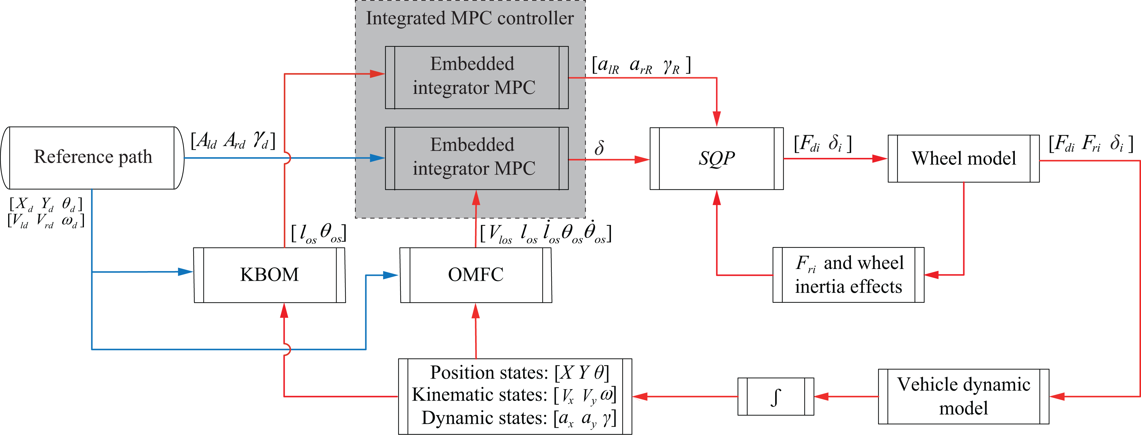
Overall flow chart for the closed-loop control of the vehicle system.

Results and discussion

In this section, the whole system mentioned earlier is simulated. Firstly, the simulation setup including the reference path and the parameters of system are introduced. Then, the simulation results are presented and discussed in detail. To indicate the advantage of the integrated MPC approach, a comparison has been made with the kinematic-based MPC algorithm implemented in the path tracking.

Simulation setup

To test the effect of the 2WS4WD vehicle system, a reference path has been generated based on a seven-order Bézier curve referring to Dai and Katupitiya.¹³ As shown in Figure 6, the path is presented in Figure 6(a), while other properties of the reference path are illustrated in Figure 6(b) to (d) which denote the path curvature, reference velocities, and accelerations, respectively. In Figure 6(a), the start point is on the reference path and defined as the origin of the global coordinate frame. The drive direction of the reference path is in the clockwise direction. In Figure 6(b), we can see that the curvature of each curved segment is less than 0.2 m⁻¹ and the fourth curved segment is the sharpest cornering of all. Figure 6(c) shows that the reference longitudinal velocity is set to around 3 m s⁻¹ and the desired lateral velocity is zero.

Figure 6.

(a) Reference path, (b) the curvature of the reference path, (c) the reference velocities, and (d) the reference accelerations.

The initial heading is set equal to the direction of the tangent to the reference path at the start point so that both the initial offset error and heading error are zero. To test the longitudinal velocity adjustment ability of the controller, the initial longitudinal velocity is set to be 0.5 m s⁻¹. While other initial velocities and accelerations are all set to zero. The system has been simulated in MATLAB using the full dynamic model of 2WS4WD vehicle, following the parameters listed in Table 1.

Table 1.

Parameters used in the simulations.

Parameter	Meaning	Value	Parameter	Meaning	Value
M	Mass of the vehicle body	200 kg	J	Inertia of the vehicle body	100 kg m²
L_f	Length of the vehicle body	0.85 m	L_r	Length of the vehicle body	0.85 m
L_h	Half width of the vehicle body	0.5 m	R_w	Radius of the wheel	0.25 m
F _dmax	Maximum drive force	1000 N	ΔF _dmax	Maximum variation of F_d within Δt	0.5 N
δ _max	Maximum steering angle	45°	Δδ _max	Search range of the steering angle	0.5°

Simulation result

The path tracking result is shown in Figure 7. In Figure 7(a), we can see that the actual path stays close to the reference path. The offset error and the heading error presented in Figure 7(b) are less than 5 cm and 8°, respectively.

Figure 7.

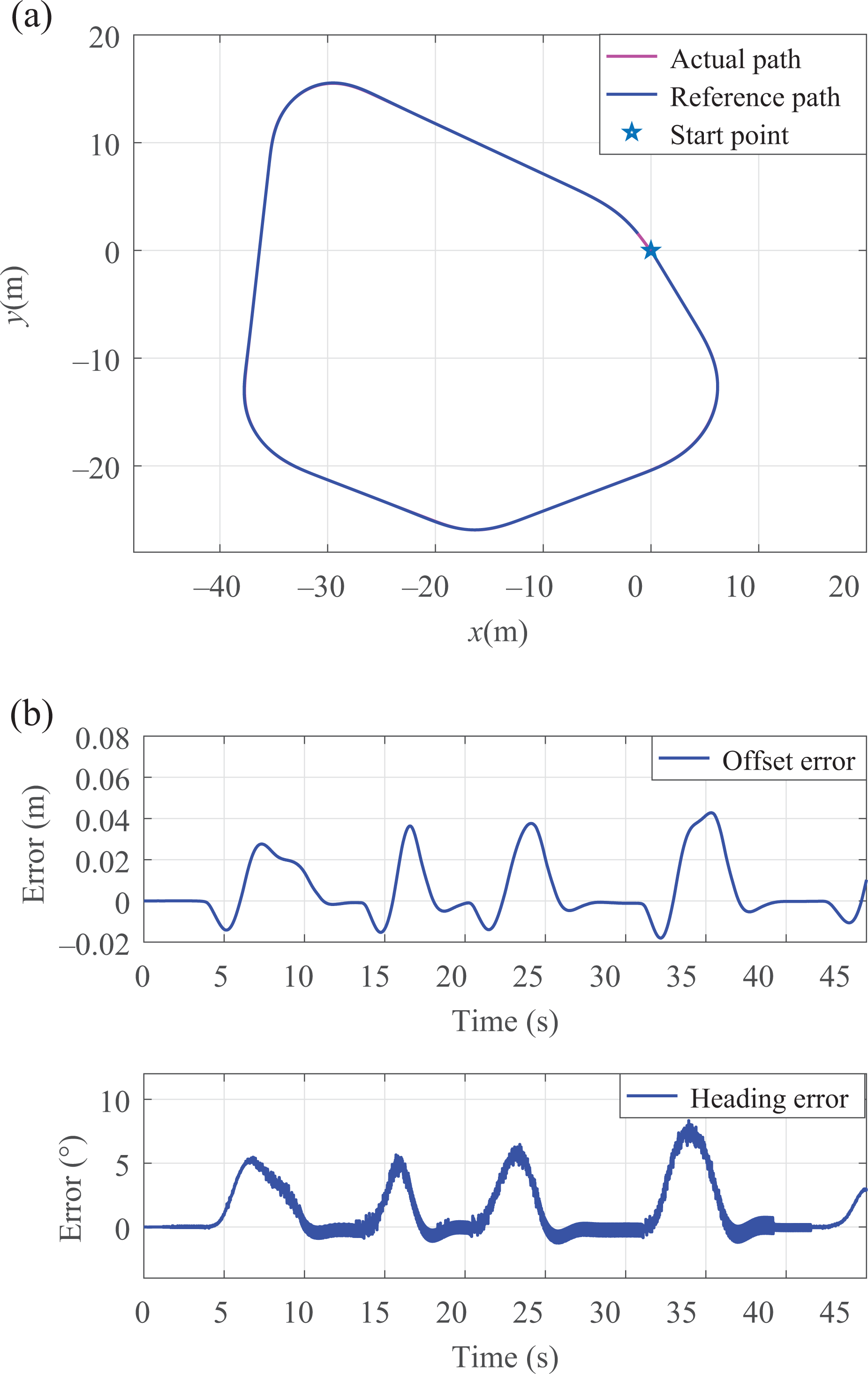
(a) Path tracking result and (b) path tracking errors.

As shown in Figure 8, the reference steering angle undergoes smooth changes along the path which demonstrates that the kinematic-based MPC part in the integrated MPC controller is reliable. For the actual steering angles, they are searching around the reference steering angle. It can be seen that the steering angles stay around zero when the path is straight and reach a negative value at cornering. Note that all cornering on this path were turning towards right. Hence, the actual steering angles of both sides have provided the correct orientation of the path tracking.

Figure 8.

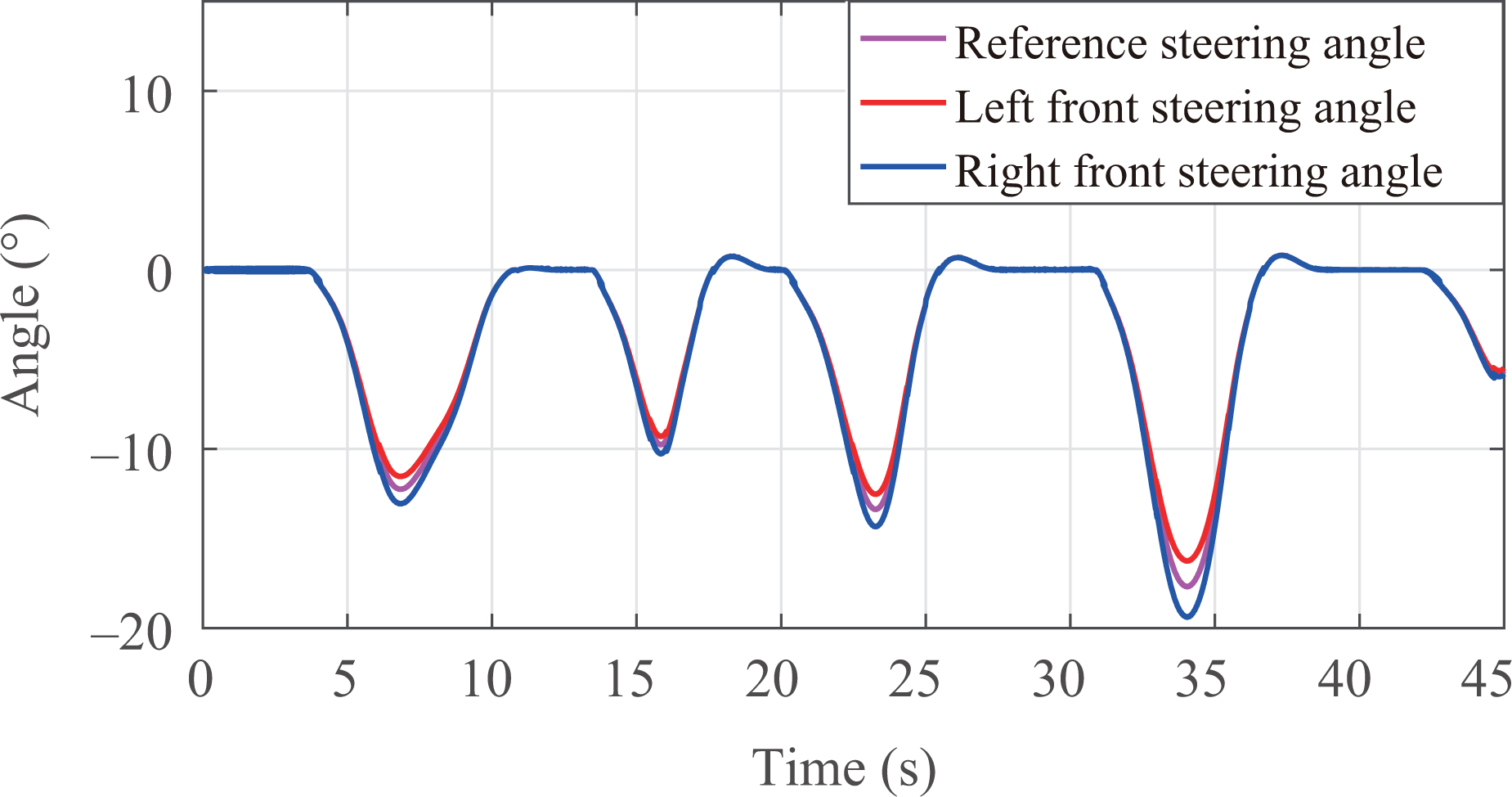
Steering angles.

In order to analyze the force control effect, the actual forces on each wheel are illustrated in Figure 9. According to Figure 9(a) and (d), the drive forces which are applied at outside wheels (i = 1, 4) increase first and then decrease when the vehicle is turning to the right. At the end of the turning, the drive forces at outside wheels reach a negative value and then return to zero, which is a result of compensatory behavior to combat the heading errors. For the inside wheels (i = 2, 3) presented in Figure 9(b) and (c), the drive forces show a behavior to the contrary of that of the outside wheels. The differential drive forces between the outside and inside wheels can provide the angular acceleration when the vehicle is turning.

Figure 9.

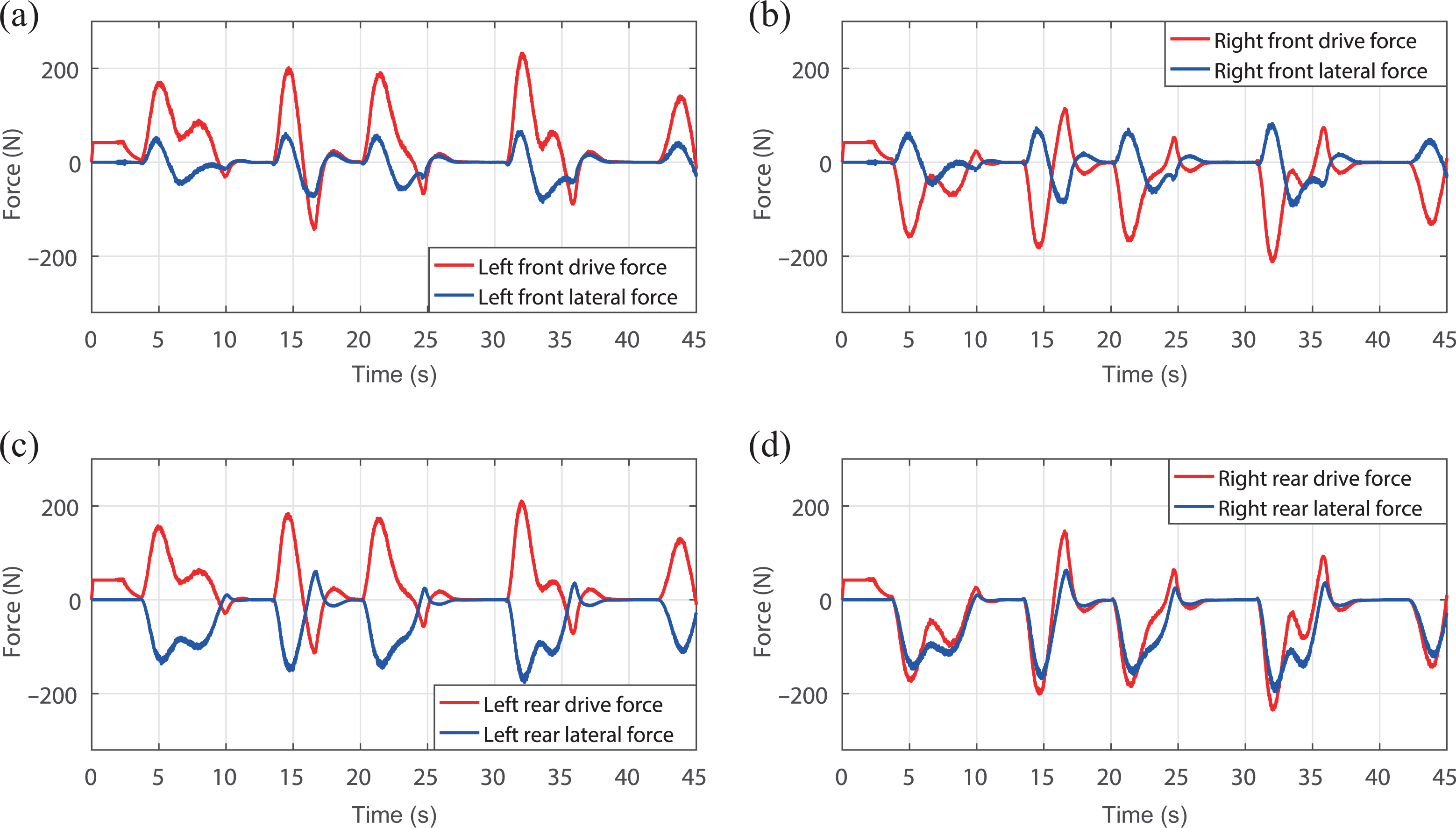
Actual forces on each wheel, (a) forces on left front wheel, (b) forces on right front wheel, (c) forces on left rear wheel, and (d) forces on right rear wheel.

The lateral forces of rear wheels shown in Figure 9(c) and (d) show smooth changes at each cornering, providing the necessary centripetal acceleration. It is because the rear wheels are nonsteerable, and the slip angles of rear wheels are equal to their corresponding side slip angles which are only related to the resultant velocity directions of each wheel. For the front wheels, it can be seen in Figure 9(a) and (b) that the lateral forces vary from −80 N to 80 N. It is because the lateral forces on the front wheels are not only based on the resultant velocity directions but also decided by the steering angles presented earlier.

Figure 10 illustrates the kinematic and the dynamic properties of the path following result. In the plots, reference velocities are the properties of the predefined path, while the virtual accelerations are the control inputs calculated by the MPC. The comparison between virtual and actual accelerations can illustrate the effect of control allocation.

Figure 10.

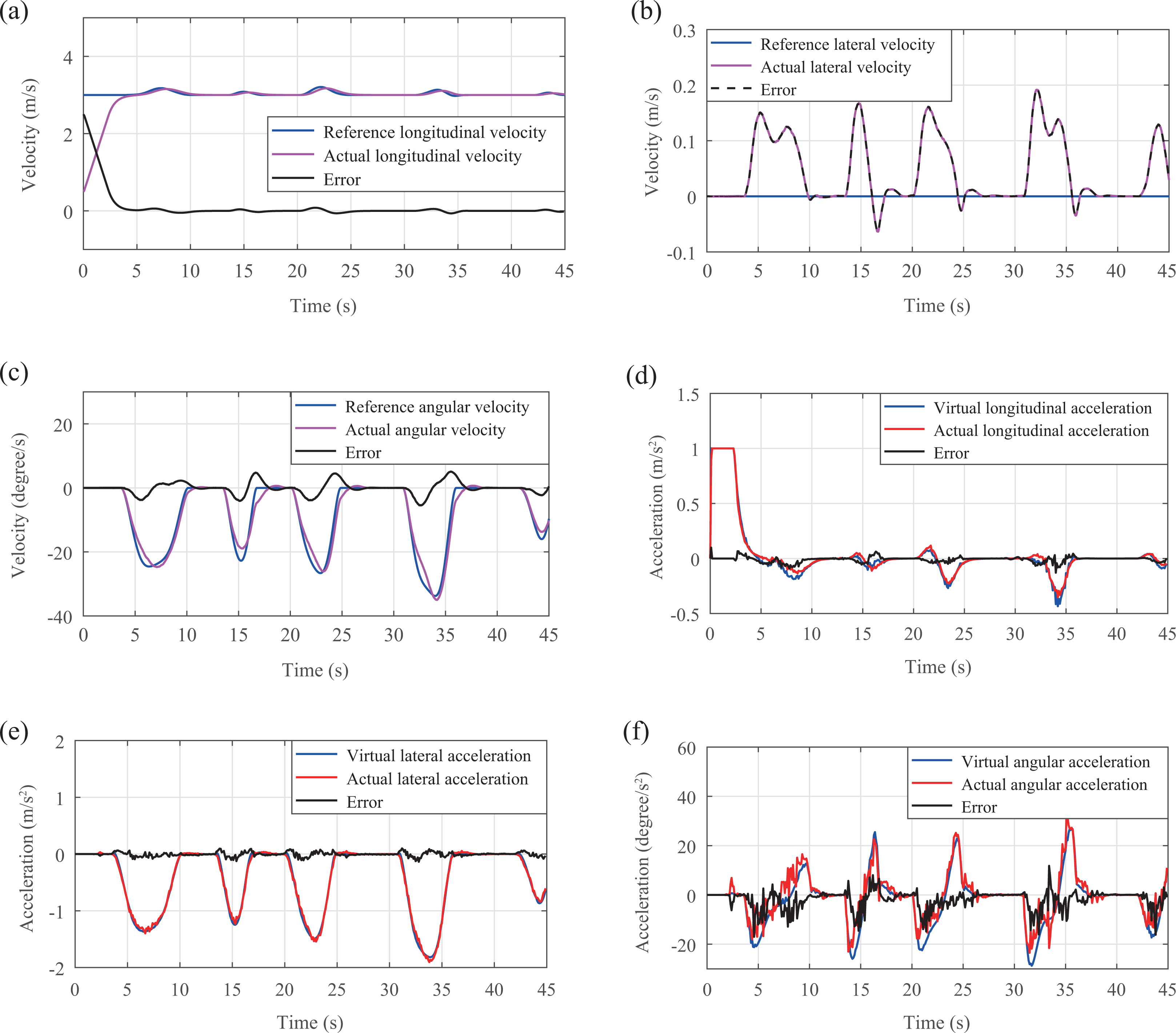
Kinematic and dynamic properties, (a) longitudinal velocity, (d) longitudinal acceleration, (b) lateral velocity, (e) lateral acceleration, (c) angular velocity, and (f) angular acceleration.

In Figure 10(a), the actual longitudinal velocity of the vehicle starts increasing from 0.5 m s⁻¹ to 3 m s⁻¹ in 3 s and then keeps stable around 3 m s⁻¹ following the reference longitudinal velocity. The velocity shown in Figure 10(b) is the lateral velocity at rear wheels, from which we can see the slip velocity of the vehicle is less than 0.2 m s⁻¹ which is less than 7% of the longitudinal velocity. Thus, the slip motion of the vehicle is under controllable range. Figure 10(c) shows that the angular velocity is smoothly following the reference, demonstrating the stability during turning. In Figure 10(d) and (e), the longitudinal and lateral accelerations are illustrated. In this simulation, the actual acceleration is generated by applying F_d , F_L , and δ to the dynamic model. As is shown in the plots, the actual accelerations basically track the virtual accelerations with its errors less than 0.1 m s⁻². Thus, the SQP-based control allocation method is proved to be effective in longitudinal and lateral directions. For the angular acceleration shown in Figure 10(f), the error between actual and virtual accelerations is chattering within −15 to 10 ° s⁻² at each cornering. It is caused by the slack variables defined in the objective function of SQP. Comparing Figure 10(c) and (f), the effect of the acceleration error is basically eliminated in the process of integrating which illustrates that the control allocation is useful in the rotating direction. From all the above, the effectiveness of proposed control allocation method is demonstrated. Since the actual velocities can track their references when applying the virtual inputs calculated by the MPC, the Lyapunov stability of the system is achieved.

In order to verify the performance of SQP-based optimizer, Figure 11 is presented which contains the iteration and optimality of the optimizer. Figure 11(a) illustrates that the iteration of each sampling time varying between 5 and 35 and its average is 20, which means the optimizer converges rapidly during the whole process. Based on the Karush-Kuhn-Tucker (KKT)-optimality conditions, the Lagrange function values in Figure 11(b) show that SQP-based optimizer is always convergent.

Figure 11.

Performance of the SQP-based optimizer, (a) iterations of SQP and (b) optimality of SQP. SQP: sequential quadratic programming.

Comparison

In this section, a comparison is made between two different control approaches, namely, the kinematic model-based MPC and the one presented in this article as integrated MPC, which combines kinematic and dynamics of the vehicle. The kinematic-based MPC is based on the controller presented by Taghia et al.²⁵ Simulation of these two approaches is presented and discussed in the following.

Offset and heading errors for both control approaches are shown in Figure 12(a) and (b), respectively. The red lines denote the kinematic-based MPC, while the blue lines denote the integrated MPC. The comparison began from 6 s when the two vehicles are operating in the same velocity of 3 m s⁻¹. Based on the figures, we can see the offset error of the kinematic-based MPC may reach 0.2 m at cornering segments and no matter at the straight segments or the cornering segments, and vibrations would occur with an average range ±0.03 m. While the offset error of the integrated MPC is less than 0.05 m at cornering segments and shows a smooth changing during the operation especially in the straight segments, the offset error can be reduced and the vehicle can follow the path accurately. In Figure 12(b), the heading error of the kinematic model-based MPC can reach 20 at the fourth cornering, while the heading error of the integrated MPC reaches 6° at most which is much smaller than that of the kinematic model-based MPC. It is clear that the integrated MPC approach presented in this article has a better control effect than the kinematic-based MPC in path tracking.

Figure 12.

Error comparison between integrated MPC and kinematic-based MPC, (a) offset error comparison and (b) heading error comparison. MPC: model predictive control.

Conclusions

In this article, a control approach that combines an integrated MPC and an SQP-based control allocation method is presented to control the ground vehicle path tracking system. The stability of proposed method is proved based on the Lyapunov’s method. In this system, all the inputs are considered based on dynamic model. The lateral forces and slip motions can be measured via the wheel model. The simulation result shows that all the virtual inputs obtained from the MPC controller are reasonable and can be accurately tracked by the actual accelerations generated from the actual inputs. By applying the actual inputs obtained from the SQP optimization, the vehicle can track the reference path closely as well as keep its velocities stable. Compared with a kinematic-based MPC algorithm, the result shows a significant improvement in errors. Thus, the new control approach is proved to be effective and reliable in controlling the ground vehicle to track a predefined path. The contribution of this work is to provide a feasible solution which combines kinematic-based and dynamic-based methods to realize the precise path tracking of a 2WS4WD vehicle. In the future work, the robustness of the MPC will be considered to overcome the unpredicted force disturbances from the ground. Also, the experiments will be carried out to verify the validity of the proposed methods.

Footnotes

Authors’ note

This work is carried out at the School of Mechanical and Manufacturing Engineering, University of New South Wales, Sydney NSW 2052, Australia.

Acknowledgements

The authors would like to appreciate for the facility and assistance provided by the Group of robotics and autonomous systems, University of New South Wales.

Declaration of conflicting interests

The author(s) declared no potential conflicts of interest with respect to the research, authorship, and/or publication of this article.

Funding

The author(s) disclosed receipt of the following financial support for the research, authorship, and/or publication of this article: This work is supported by the China Postdoctoral Science Foundation (grant no 2016M600910) and the Fundamental Research Funds for the Central Universities (grant nos 2015JBC022 and 2017JBM051).

References

Guo

Yang

. Intelligent vehicle trajectory tracking based on neural networks sliding mode control. In: 2014 International conference on informative and cybernetics for computational social systems (ICCSS) (ed FY

Wang

), Qingdao, Shandong, China, 9–10 October 2014, pp. 57–62. NY, USA: IEEE.

Pacheco

Luo

. Testing PID and MPC performance for mobile robot local path-following. Int J Adv Robot Syst 2015; 12: 1–13.

Urrea

Muñoz

. Mobile robot based on the selection of fuzzy behaviours for following trajectories in crops. Int J Adv Robot Syst 2016; 13(3): 1–10.

Zhou

Wang

. Robust sliding mode control of 4WS vehicles for automatic path tracking. In: Proceedings of 2005 IEEE intelligent vehicles symposium, Las Vegas, NV, USA, 6–8 June 2005, pp. 819–826. NY, USA: IEEE.

Taghia

Katupitiya

. Wheel slip identification and its use in the robust control of articulated offroad vehicles. In: Proceedings of 2013 Australasian conference on robotics and automation (ed J

Katupitiya

), Sydney, Australia, 2–4 December 2013, pp. 1–9. Australia: Australian Robotics and Automation Association (ARAA).

Fang

Fan

Thuilot

. Trajectory tracking control of farm vehicles in presence of sliding. Robot Auton Syst 2006; 54(10): 828–839.

Lenain

Thuilot

Cariou

. Model predictive control for vehicle guidance in presence of sliding: application to farm vehicles path tracking. In: Proceedings of 2005 IEEE international conference on robotics and automation (ICRA), Barcelona, Spain, 18–22 April 2005, pp. 885–890. NY, USA: IEEE.

Lenain

Thuilot

Cariou

. High accuracy path tracking for vehicles in presence of sliding: application to farm vehicle automatic guidance for agricultural tasks. Auton Robot 2006; 21(1): 79–97.

Alfi

Farrokhi

. Hybrid state-feedback sliding-mode controller using fuzzy logic for four-wheel steering vehicles. Vehicle Syst Dyn 2009; 47(3): 265–284.

10.

Lucet

Lenain

Grand

. Dynamic path tracking control of a vehicle on slippery terrain. Control Eng Pract 2015; 42: 60–73.

11.

Peng

. On one approach to constraining the combined wheel slip in the autonomous control of a 4ws4wd vehicle. IEEE Trans Control Syst Technol 2007; 15(1): 168–175.

12.

Oyelere

. The application of model predictive control (mpc) to fast systems such as autonomous ground vehicles (agv). IOSR J Comput Eng 2014; 16(3): 27–37.

13.

Dai

Katupitiya

. Path planning and force control of a 4WD4WS vehicle. In: Proceedings of Australasian conference on robotics and automation (ed D

Oetomo

), Sydney, Australia, 2–4 December 2014, pp. 1–10. Australia: Australian Robotics and Automation Association (ARAA).

14.

Ono

Hattori

Muragishi

. Vehicle dynamics integrated control for four-wheel-distributed steering and four-wheel-distributed traction/braking systems. Vehicle Syst Dyn 2006; 44(2): 139–151.

15.

Yang

Cocquempot

Jiang

. Optimal fault-tolerant path-tracking control for 4WS4WD electric vehicles. IEEE Trans Intell Transp Syst 2010; 11(1): 237–243.

16.

Dai

Katupitiya

. Online path tracking and motion optimization of a 4WS4WD vehicle. In 2015 IEEE/RSJ international conference on intelligent robots and systems (IROS) (ed J

Zhang

), Hamburg, Germany, 28 September–2 October 2015, pp. 4133–4139. NY, USA: IEEE.

17.

Roberge

Tarbouchi

Labonté

. Comparison of parallel genetic algorithm and particle swarm optimization for real-time UAV path planning. IEEE Trans Ind Inform 2013; 9(1): 132–141.

18.

Simmons

. Control allocation techniques using existing and novel quadratic programming algorithms. Auburn, Alabama, USA: Master’s Thesis of Auburn University, 2003, pp. 35–45.

19.

Johansen

Fossen

TI,

Berge

. Constrained nonlinear control allocation with singularity avoidance using sequential quadratic programming. IEEE Trans Control Syst Technol 2004; 12(1): 211–216.

20.

Woods

Katupitiya

. Modelling of a 4WS4WD vehicle and its control for path tracking. In: 2013 IEEE Symposium on computational intelligence in control and automation (CICA), Singapore, Singapore, 16–19 April 2013, pp. 155–162. NY, USA: IEEE.

21.

Huynh

Katupitiya

Kwok

. Derivation of an error model for tractor-trailer path tracking. In: 2010 International conference on intelligent systems and knowledge engineering (ISKE), Hangzhou, China, 15–16 November 2010, pp. 60–66. NY, USA: IEEE.

22.

Timings

Cole

. Minimum maneuver time calculation using convex optimization. J Dyn Syst Meas Control 2013; 135(3): 031015.

23.

Wang

. Model Predictive Control System Design and Implementation using Matlab®. New York, NY, USA: Springer Science & Business Media, 2009.

24.

Khalil

. Nonlinear Systems, 3rd ed. Upper Saddle River, NJ: Prentice-Hall, 2002.

25.

Taghia

Wang

Lam

. A sliding mode controller with a nonlinear disturbance observer for a farm vehicle operating in the presence of wheel slip. Auton Robot 2017; 41(1): 71–88.

Force control of two-wheel-steer four-wheel-drive vehicles using model predictive control and sequential quadratic programming for improved path tracking

Abstract

Keywords

Introduction

Vehicle system modeling

Vehicle kinematic model

Model description

Kinematic model-based offset model

Vehicle dynamic model

Model description

Offset model for the force control

Wheel model

Control algorithm and its implementation

Embedded integrator MPC

Control design

Stability proof

Remark 3.1

Theorem 3.1

Proof

Control allocation

Sequential quadratic programming

Closed-loop control of the vehicle system

Results and discussion

Simulation setup

Simulation result

Comparison

Conclusions

Footnotes

Authors’ note

Acknowledgements

Declaration of conflicting interests

Funding

References