Sage Journals: Discover world-class research

Abstract

In this article, a dynamical model for controlling an omniwheel mobile robot is presented. The proposed model is used to construct an algorithm for calculating control actions for trajectories characterizing the high maneuverability of the mobile robot. A description is given for a prototype of the highly maneuverable robot with four omniwheels, for which an algorithm for setting the coefficients of the PID controller is considered. Experiments on the motion of the robot were conducted at different angles, and the orientation of the platform was preserved. The experimental results are analyzed and statistically assessed.

Keywords

Omniwheel mobile robot dynamical model PID controller experimental investigations

Introduction

Highly maneuverable mobile robots are widely used as service robots, transportation robots, footballer robots, and so on; see the litereature^1

–9 for a detailed analysis of the robots’ designs and experience of their applications. Also there are publications described dynamical theory with the effects of slip.^10,11 Maneuverability is an important property of mobile robots, since more maneuverable robots have advantages under limited space conditions. One of the ways to ensure a high maneuverability of the robot is to use omniwheels,^12,13 which, when properly arranged, allow the robot to move in any direction without reorientation. Recently, many scientists have been engaged in developing various kinematic schemes of omniwheel robots and their control algorithms,^14,15 including spherical robots, when the platform with omniwheels is placed inside a spherical shell.^16,17

In spite of a large number and variety of publications devoted to omniwheel mobile robots, no experimental results have been presented to demonstrate their maneuverability. Most articles present only the results of numerical simulations, while the examples given in them are in fact those of simple trajectories of motion. The aim of this article is to evaluate the experimental trajectories of an omniwheel mobile robot preserving its orientation and to consider the particularities of implementation of control for the execution of complicated maneuvers.

The nonholonomic model of an omniwheel

We recall that such a wheel has rollers fastened on the periphery (outer rim), so that only one of the rollers of the wheel is in contact with the supporting surface. Each roller rotates freely about the axis which is fixed relative to the plane of the disk, and the wheel can roll in a straight line which makes a fixed angle with the plane of the wheel. For Mecanum wheels, the roller axis is fastened at an angle of 45° to the plane of the wheel, whereas for most omniwheels, the roller axis lies in the plane of the wheel. The simplest nonholonomic model of an omniwheel is a flat disk for which the velocity of the point of contact with the supporting surface is directed along a straight line which forms a constant angle δ with the plane of the wheel (see Figure 1).

Figure 1.

The schematic and the nonholonomic model of an omniwheel.

Let τ and n be the tangent and normal vectors to the plane of the wheel at the point of contact, such that the vector τ × n is directed vertically upward, and let α be the unit vector along the axis of attachment of the rollers. Then, the constraint equation is

(V_{Q}, α) = 0

where V _Q is the velocity of the point of contact. If V _O is the velocity of the center of the wheel and ψ is the angle of the wheel’s rotation (measured counterclockwise when viewed from the tip of the vector n ), then the constraint equation can be rewritten as

(V_{O} + h \dot{ψ} τ, α) = 0

where h is the radius of the wheel. It is convenient to solve this equation for $\dot{ψ}$ , whence

\dot{ψ} = - \frac{1}{s h} (V_{O}, α), s = (α, τ) = sin δ

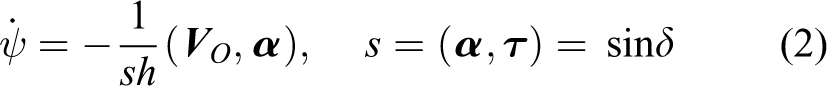
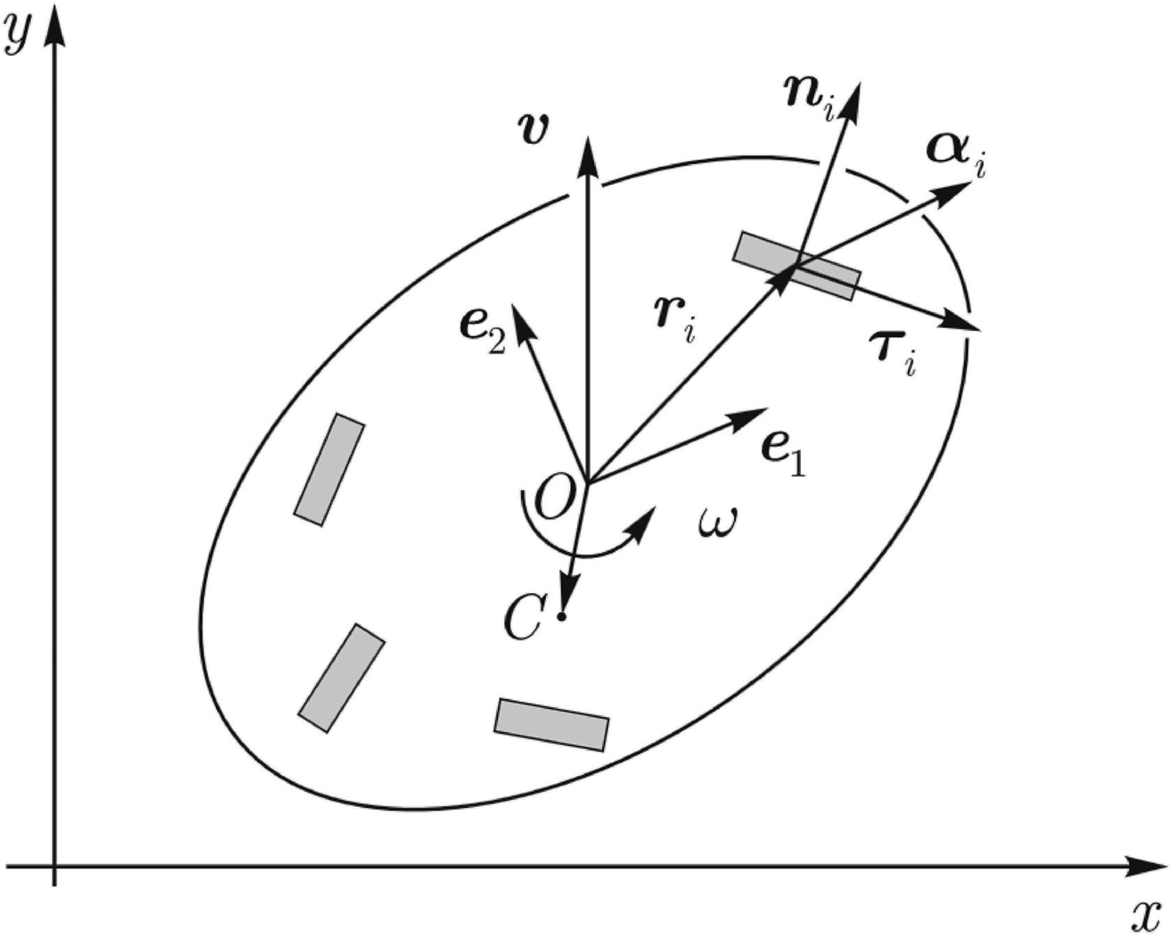
Since the vector α is defined up to the sign, one may assume without loss of generality that s ≥ 0.

An omniwheel mobile robot

We obtain the equations of motion for an omniwheel mobile robot rolling on a horizontal plane and consisting of a platform (framework), to which an arbitrary number of wheels is attached in such a way that their axes are fixed relative to the platform (Figure 2).

Figure 2.

Schematic of an omniwheel mobile robot.

Choose a moving coordinate system $O e_{1} e_{2}$ rigidly attached to the platform. Let x, y, and ϕ denote the coordinates of the origin O and the angle of rotation of the axes e ₁ and e ₂ about the fixed coordinate system, respectively. The vectors $r_{i}, τ_{i}, α_{i}, i = 1, \dots, n$ , specifying the position, plane, and direction of the roller axis of each wheel are constant in the moving axes. Let $v = (v_{1}, v_{2})$ denote the velocity of the origin O of the moving coordinate system which is referred to the moving axes, and let ω be the angular velocity of the platform. Then, the constraint equation (2) defining the direction of the velocities of the contact points can be written as

f_{i} = {\dot{ψ}}_{i} + G_{i}, G_{i} = \frac{1}{s_{i} h_{i}} (v + ω J r_{i}, α_{i}), J = (\begin{matrix} 0 & - 1 \\ 1 & 0 \end{matrix})

The vector $ω J r_{i}$ in the three-dimensional space corresponds to the vector product of the form ω × r _i, where ω = (0, 0, ω).

With no constraints imposed, the kinetic energy of the system consists of the kinetic energy of the platform

T_{0} = \frac{1}{2} m_{0} v^{2} + \frac{1}{2} I_{0} ω^{2} + m_{0} ω (J R_{o c}, v)

where m₀ is the mass of the framework, I₀ is its moment of inertia relative to the point O, and R _oc is the vector OC ( C is the center of mass of the platform) and the kinetic energy of each of the wheels

T_{i} = \frac{1}{2} m_{i} (v + ω J r_{i}, v + ω J r_{i}) + \frac{1}{2} I_{i} {\dot{ψ}}_{i}^{2} + \frac{1}{2} {\tilde{I}}_{i} ω^{2}

where m_i is the mass of the ith wheel, and I_i and ${\tilde{I}}_{i}$ are the central moments of inertia of the wheel relative to the axis and the diameter, respectively. Here and in the sequel, we assume that the centers of mass of the wheels lie on their axes, and the mass distribution of the wheel possesses axial symmetry, that is, the central tensor of inertia of the wheel has the form $I_{i} = diag (I_{i}, {\tilde{I}}_{i}, {\tilde{I}}_{i})$ . For the total kinetic energy, we finally obtain

\begin{matrix} T = T_{0} + \sum_{i = 1}^{n} T_{i} = \frac{1}{2} m v^{2} + \frac{1}{2} I ω^{2} + m ω (J r_{c}, v) + \frac{1}{2} \sum_{i} I_{i} {\dot{ψ}}_{i}^{2} \end{matrix}

where

$m = m_{0} + \sum_{i} m_{i}$ is the total mass of the system

I = I_{0} + \sum_{i} m_{i} r_{i}^{2} + {\tilde{I}}_{i}

is the total moment of inertia relative to the point O, and

r_{c} = m^{- 1} (m_{0} R_{o c} + \sum_{i} m_{i} r_{i})

is the center of mass of the entire system.

In this approach, we neglect the inertia of the rollers.

We write for this system the equations of motion in quasivelocities with undetermined multipliers in the form

\begin{matrix} {(\frac{\partial T}{\partial v})}^{\cdot} + ω J \frac{\partial T}{\partial v} = \sum_{k} λ_{k} \frac{\partial f_{k}}{\partial v} = \sum_{k} λ_{k} \frac{\partial G_{k}}{\partial v}, \\ {(\frac{\partial T}{\partial ω})}^{\cdot} + (J v, \frac{\partial T}{\partial v}) = \sum_{k} λ_{k} \frac{\partial f_{k}}{\partial ω} = \sum_{k} λ_{k} \frac{\partial G_{k}}{\partial ω}, \\ {(\frac{\partial T}{\partial {\dot{ψ}}_{i}})}^{\cdot} = λ_{i} + M_{i}, i = 1, \dots, n \end{matrix}

where M_i is the moment of forces applied to the axes of the wheels.

From the last equation and the constraint equation (3), we find the undetermined multipliers in the form

λ_{i} = - I_{i} {\dot{G}}_{i} - M_{i} = - \frac{I_{i}}{s_{i} h_{i}} (\dot{v} + \dot{ω} J r_{i}, α_{i}) - M_{i}

Substituting them into the first two equations and adding the kinematic relations governing the motion of the moving axes $O e_{1} e_{2}$ , we obtain a complete system of equations of motion in the form

(Γ + m E) \dot{v} + m \dot{ω} (J r_{c} + R) + m ω J (v + ω J r_{c}) = - \sum_{i} μ_{i} α_{i}, \hat{I} \dot{ω} + m (J r_{c} + R, \dot{v}) + m ω (v, r_{c}) = - \sum_{i} μ_{i} (J r_{i}, α_{i}), \dot{x} = v_{1} cos ϕ - v_{2} sin ϕ, \dot{y} = v_{1} sin ϕ + v_{2} cos ϕ, \dot{ϕ} = ω, Γ = \sum_{i} \frac{I_{i}}{s_{i}^{2} h_{i}^{2}} α_{i} \otimes α_{i}, R = m^{- 1} \sum_{i} \frac{I_{i}}{s_{i}^{2} h_{i}^{2}} (J r_{i}, α_{i}) α_{i}, \hat{I} = I + \sum_{i} \frac{I_{i}}{s_{i}^{2} h_{i}} {(J r_{i}, α_{i})}^{2}, μ_{i} = \frac{M_{i}}{s_{i} h_{i}}

where E is the identity matrix.

Recall that the tensor product of the vectors a and b is defined as follows

a \otimes b = ∥ a_{i} b_{j} ∥

Note that the matrix Γ is degenerate if and only if all vectors α _i are parallel to each other; otherwise, Γ is nondegenerate.

If the moments of forces μ_i applied to the wheel axes have the form $μ_{i} = ω {\bar{μ}}_{i}$ , where ${\bar{μ}}_{i}$ is independent of v and ω, then equation (5) admits the singular invariant measure.¹⁸

μ = \frac{1}{ω} d v_{1} d v_{2} d ω d x d y d ϕ

Arbitrariness in the choice of the origin and the rotation of the moving axes can be used in order to simplify either the equations of motion or the integrals of the system (if any).

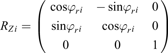
Description of a prototype of the omniwheel robot

The use of an omniwheel in designing mobile robots allows one to develop various designs. The most widespread are robots having three or four omniwheels,^1,4,7,10,11 but there exist mobile robots with six omniwheels.¹⁹ The design of the omniwheel can also be different.² First of all, this concerns the shape of the rollers, their number, the way of attachment to the rim, and the angle between the axis of rotation of the roller and the plane of the wheel.

The omniwheel mobile robot dealt with in this article is a prefabricated structure whose basis is an articulated platform (consisting of two semiplatforms) to which four omniwheels of Mecanum type (1) with actuators are fastened (the rollers on the wheels are arranged at an angle of 45° to the wheel’s axis). The semiplatforms of the robot are fastened to each other only in the central part, which allows the wheel pairs to move relative to each other in the vertical plane. This ensures constant contact of all four wheels with the supporting surface during the motion on a rough surface. Each of the wheels is equipped with an individual actuator, so that the most diverse combinations of directions and rotational velocities of the wheels can be given. Coupled with the special structure of the wheels, this enables fairly complicated motions of the mobile robot on the plane. Each wheel actuator has a feedback sensor (encoder), which makes it possible to keep track of the real rotational velocity of the wheel and to precisely maintain the given velocity of rotation by means of the PID controller. The platform has a control card, which includes a microcontroller with a control system, motor drivers, and wireless communication units.

An experimental model of the robot is shown in Figure 3.

Figure 3.

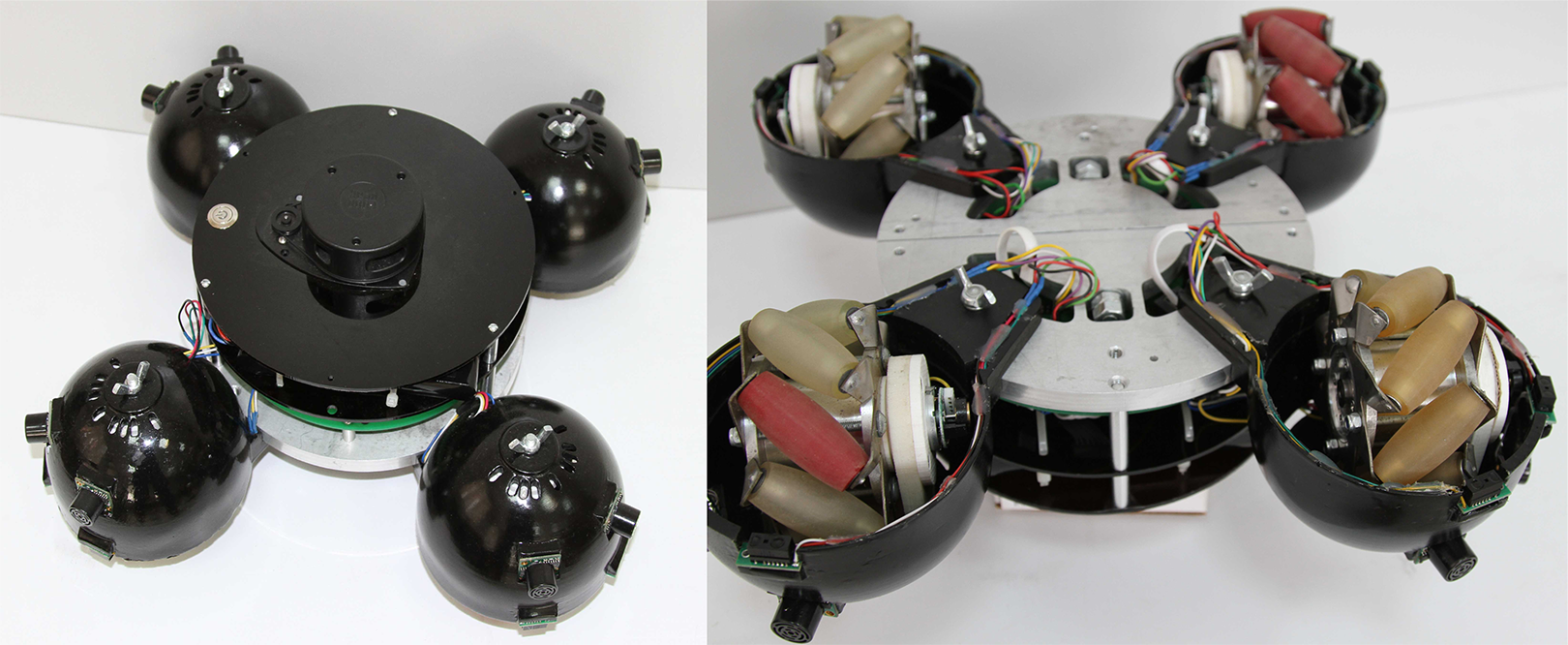
Experimental model of an omniwheel robot.

The control is implemented from a personal computer, for which special software has been developed. All control commands are transmitted via a wireless communication channel. The velocity values of each of the wheels and the direction of their rotation, which are precalculated depending on the given trajectory, are transmitted to the robot in one data package.

The developed design is defined by the vectors $r_{i}, α_{i}, and τ_{i}$ for each wheel, where i = 1, 2, 3, 4 is the index denoting the number of the corresponding wheel.

For the vector r _i, we introduce a matrix of rotation relative to the axis Z through the angle ϕ_i

R_{Z}_{i} = (\begin{matrix} cos ϕ_{r}_{i} & - sin ϕ_{r}_{i} & 0 \\ sin ϕ_{r}_{i} & cos ϕ_{r}_{i} & 0 \\ 0 & 0 & 1 \end{matrix})

where ϕ_ri is the angle between the axis x and the vector r _i. Then, the vector r _i is

r_{i} = (\begin{matrix} H \\ 0 \\ 0 \end{matrix}) \cdot R_{Z}_{i}

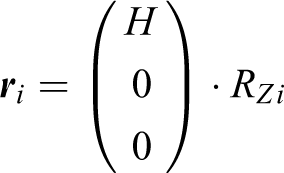
where H is the distance from the center of the platform to the center of the wheel.

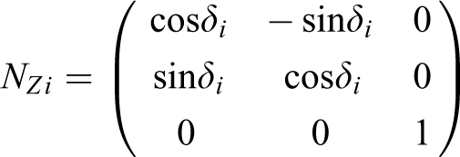
For the vector n _i, we introduce a matrix of rotation through angle δ_i

N_{Z}_{i} = (\begin{matrix} cos δ_{i} & - sin δ_{i} & 0 \\ sin δ_{i} & cos δ_{i} & 0 \\ 0 & 0 & 1 \end{matrix})

where δ_i is the angle between the vectors r _i and n _i. Then, the vector n _i is

n_{i} = (\begin{matrix} 1 \\ 0 \\ 0 \end{matrix}) \cdot N_{Z}_{i} \cdot R_{Z}_{i}

For the vector α _i, we introduce matrices of rotation through angle ξ_i

A_{Z}_{i} = (\begin{matrix} cos ξ_{i} & - sin ξ_{i} & 0 \\ sin ξ_{i} & cos ξ_{i} & 0 \\ 0 & 0 & 1 \end{matrix})

where ξ_i is the angle defining the type of wheel (left or right). For the left wheel, ξ = 45°, and for the right wheel, ξ = 135°. Then, the vector α _i is

α_{i} = (\begin{matrix} 1 \\ 0 \\ 0 \end{matrix}) \cdot A_{Z}_{i} \cdot N_{Z}_{i} \cdot R_{Z}_{i}

A diagram of a four-wheeled robot with denoted vectors and angles is presented in Figure 4.

Figure 4.

An example of how the vectors and angles are denoted for a four-wheeled omniwheel robot.

The design of the omniwheel robot is determined by the following geometrical parameters: the number of wheels N = 4, h = 0.0475 m, H = 0.16 m, ϕ₁ = 45°, ϕ₂ = 135°, ϕ₃ = 225°, ϕ₄ = 315°, δ₁ = δ₃ = −45°, δ₂ = δ₄ = 45°, ξ₁ = ξ₃ = 45°, and ξ₂ = ξ₄ = 135°. Further calculations will be performed for these parameter values.

Algorithm for selecting the parameters of a PID controller

A given rotational velocity of each wheel is reached by means of a PID controller. It adjusts the control actions for each motor depending on the load and ensures a constant rotational speed. For an efficient operation of the PID controller, it is necessary to select values of the coefficients of the PID controller, K_p, K_i, and K_d, for a specific object of regulation. There is a large body of published research on the use of PID controllers in mobile robots and there exist various methods for selecting its coefficients.^6,7

The PID controller of the omniwheel mobile robot presented here controls the off-duty ratio of the PWM signal applied to each motor. Synchronization with the preset value occurs with a frequency of 200 Hz.

The preliminary calculation of the parameters of the PID controller has been performed using a control system model developed in the Simulink software of the MATLAB software environment. A model of the control system is presented in Figure 5.

Figure 5.

Model of a control system developed in the Simulink software of the MATLAB software environment.

The required velocity of rotation is given in the speed demand unit in revolutions per minute. In the gearbox unit, one sets the value of the reduction ratio of the reduction gear, and in the wheel and axle unit, one specifies the radius of the installed wheel for the motor shaft to ensure the possibility of simulating the system with different loads. In the DC motor unit, one specifies the parameters of the simulated commutator DC motor. The speed controller unit contains a PID speed controller; Figure 6 shows a model of a speed controller.

Figure 6.

Model of a speed controller.

The following parameters of the Pololu 30 motor reducer have been used for simulation: metal Gearmotor 37D × 68 L with characteristics presented in Table 1.

Table 1.

Characteristics of the motor reducer.

Characteristics of the motor	Symbol	Value
Rated supply voltage	U_n	12 V
Rated torque	M_l	0.78 N ⋅ m
Ohmic resistance of the armature winding	R	4.6 Ω
Inductance of the armature winding	L	15.7 mH
Equivalent moment of inertia	J	0.0001 kg m²
Rated rotational speed	n	10500 r/min
Mechanical constant	C_m	0.01115 Nm/A
Electrotechnical constant	C_e	0.053 V ⋅ s
Reduction ratio of the reduction gear	i	30

For an efficient operation of the PID controller, it is necessary to select values of the coefficients of the PID controller, K_p, K_i, and K_d, for a specific object of regulation. One of the methods of tuning the PID controller is the method of undamped oscillations or the Ziegler–Nichols method²⁰

In the operating system, the integral gain and the derivative gain of the controller are set to zero (K_i = 0, K_d = 0), that is, the system is set to the proportional law of regulation.

By successively increasing K_p, one obtains undamped oscillations for K_p = K, with period T. In this case, the system is at the boundary of oscillatory stability.

The values of K and T are fixed. When critical oscillations arise, none of the variables of the system should reach the level of limitation. The settings of the controller are calculated from the values of T and K: K_p = 0.6K, K_i = 0.83T/K, and K_d = 0.075KT.

Using the abovementioned method for this system, the following values of the coefficients of the speed controller have been obtained: K_p = 16.2, K_i = 0.307, and K_d = 19.5.

This method is rather simple but does not always give very good results. After calculation of the parameters of the controller, it is usually necessary to perform its manual fine tuning to improve the quality of regulation. For this purpose, the following experiment has been conducted:

The rotational velocity of one of the robot wheels was set to 170 r/min for 3 s.

The values of the actual velocity from the encoder were preserved with a frequency of 10 Hz when the wheel was rotated in the air without load.

A graph of the rotational velocity was plotted and used to determine the quality and the rapidity of attaining the specified velocity value. The time of the transitional process, t_set, and the average quadratic deviation of σ from the specified value after t_set were measured.

The experiment was repeated for K_p = 14.2 … 18.2 with the step 0.1, K_i = 0.1 … 0.4 with the step 0.01, and K_d = 17.5 … 21.50 with the step 0.1.

By analyzing the values of t_set and σ for each experiment, the optimal values of the coefficients of the PID controller for which t_set and σ are minimal were selected: K_p = 17.1, K_i = 0.160, and K_d = 19.3. Figure 7 shows a graph of the transitional process of rotation of the wheel with the coefficients of the PID controller: K_p = 14.2, K_i = 0.1, and K_d = 17.5 (the dashed line); K_p = 17.1, K_i = 0.16, and K_d = 19.3 (the solid line); and K_p = 18.2, K_i = 0.4, and K_d = 21.5 (the doted line).

Figure 7.

Graph of the rotational velocity of the wheel at the instant of start with different coefficients of the PID controller.

Experimental investigations

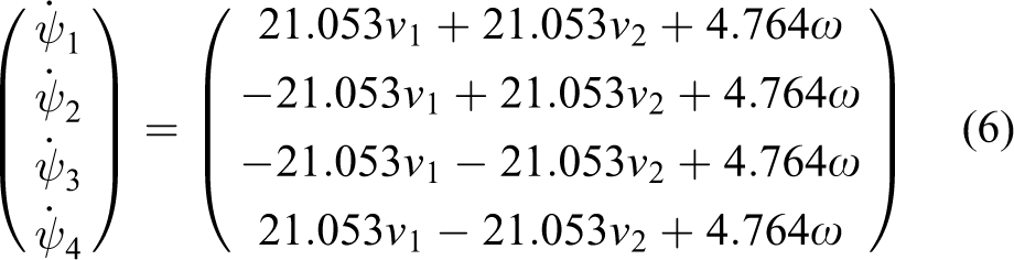
Since sensors of the angular rotational velocity are installed on the actuating motors and since we can ensure a sufficiently accurate control of the angular velocities of rotation of the omniwheels when using the PID controller, we choose the angular rotational velocities of the wheels as control actions. Then, given the geometrical characteristics and the condition of no slipping of the wheel rollers at the point of contact with the surface, the expression for calculation of the control actions looks as follows

(\begin{matrix} {\dot{ψ}}_{1} \\ {\dot{ψ}}_{2} \\ {\dot{ψ}}_{3} \\ {\dot{ψ}}_{4} \end{matrix}) = (\begin{matrix} 21.053 v_{1} + 21.053 v_{2} + 4.764 ω \\ - 21.053 v_{1} + 21.053 v_{2} + 4.764 ω \\ - 21.053 v_{1} - 21.053 v_{2} + 4.764 ω \\ 21.053 v_{1} - 21.053 v_{2} + 4.764 ω \end{matrix})

The high maneuverability of the omniwheel mobile robot is demonstrated by the following experiment. The robot moves along a straight-line trajectory for 2 s (the time value is determined by the limited space of the laboratory) with velocity V = 0.5 m/s at angles $θ = \frac{π}{6} n$ , n = 0…12, where n is the number of the experiment. The motion was started from rest, without rotating the platform of the robot: v₁ = V cosθ, v₂ = V sinθ, ω = 0, and ϕ = const. Each experiment was conducted three times under the same conditions, after which a statistical processing of data was performed.

The experiments were conducted in a laboratory equipped with a Vicon motion capture system. This system makes it possible to determine the trajectory of the robot with an accuracy of 0.1 mm. Figure 8 shows the average trajectories of the robot (solid line) with confidence intervals for a probability of 95% (the grey area along the average trajectory) for angles from 0° to 360° with a step of 30°. The average trajectories were constructed for three experiments, which were conducted under the same conditions. The graph of the theoretical trajectory is shown in dashed line.

Figure 8.

Graphs of the trajectory of the omniwheel robot.

The figure also shows schematically the mobile robot before the start of motion (at the center of the coordinate system) and after its completion so that the change in its orientation during the motion is taken into account. The greatest deviation from the given angle of orientation was 8°.

Also were conducted experiments demonstrated the high maneuverability of an omniwheeled mobile robot. There were two series of experiments when the robot moved around a circle: in the first case, the robot moved along a circle with constant orientation (ω = 0, ϕ = const). Figure 9 shows the results of the experiment moving around the circle with radius R_c = 0.65 m. In the second case, the robot moved around the circle when the speed vector was directed tangentially to the circle and the robot turned around Z-axis in the moving coordinae system one time (ω = Ω, where Ω = V/R_c is the angular velocity and R_c is the the radius of the circle). The result of the experiment in case of V = 1 m/s and R_c = 0.65 m is shown in Figure 10.

Figure 9.

Graph of the trajectory of the omniwheel robot by moving on circle with constant orientation.

Figure 10.

Graph of the trajectory of the omniwheel robot by moving on circle with rotation.

Conclusions

The research results presented in this article allow the following conclusions to be drawn.

The developed omniwheel robot can move fairly accurately at different angles without changing its orientation. The maximal deviation from the original orientation was 8° for the motion along a line at an angle of 210°. The deviations of the motion of the robot from the theoretical trajectory can be explained by the fact that the robot has DC motors, which cannot ensure that the necessary torque is reached rapidly, particularly at low rotational velocities typical of the given direction of motion. This problem is also the main reason of derivation of mobile robot in case of movement around a circle with constant orientation. Also, the theoretical model is based on the condition of no slipping of the rollers, but in practice, this is a rather complicated problem, which is not always solvable.

In the future, using the results obtained, it will be possible to make this omniwheel robot move along complex trajectories,²¹ to implement a computer vision system to bypass obstacles,^22,23 navigation systems,²⁴ and to develop a group control system for these robots.

Footnotes

Authors’ note

The work of AA Kilin (“The nonholonomic model of an omniwheel and An omniwheel mobile robot” sections) was carried out within the framework of the state assignment of the Ministry of Education and Science of Russia (1.2404.2017/4.6). The work of Yu L Karavaev and V Klekovkin (“Description of a prototype of the omniwheel robot, Algorithm for selecting the parameters of a PID controller, and Experimental investigations” sections) was carried out within the framework of the state assignment of the Ministry of Education and Science of Russia (1.2405.2017/4.6).

Author contribution

The contribution is sponsored by VEGA MS SR No 1/0367/15 prepared project “Research and development of a new autonomous system for checking a trajectory of a robot.”

Declaration of conflicting interests

The author(s) declared no potential conflicts of interest with respect to the research, authorship, and/or publication of this article.

Funding

The author(s) received no financial support for the research, authorship, and/or publication of this article.

References

Taheri

Qiao

Ghaeminezhad

. Kinematic model of a four mecanum wheeled mobile robot. Int J Comput Appl 2015; 113(3).

Byun

Song

. Design and construction of continuous alternate wheels for an omnidirectional mobile robot. J Robot Syst 2003; 20(9): 569–579.

Lin

Shih

. Modeling and adaptive control of an omni-mecanum-wheeled robot. Int Control Autom 2013; 4(2): 166.

Samani

Abdollahi

Ostadi

. Design and development of a comprehensive omni directional soccer player robot. Int J Adv Robot Syst 2004; 1(3): 20.

Doroftei

Grosu

Spinu

. Omnidirectional mobile robot–design and implementation. Austria: Intech Open Access Publisher, 2007.

Zhao

Chen

Song

. Design of a control system for an autonomous vehicle based on adaptive-PID. Int J Adv Robot Syst 2012; 9(2): 44.

Han

Choi

Kim

. Design and control of mobile robot with mecanum wheel. In: ICCAS-SICE, Fukuoka, Japan, 2009, pp. 2932–2937.

Borisov

Kilin

AA,

Mamaev

. Dynamics and control of an omniwheel vehicle. Reg Chaot Dyn 2015; 20(2): 153–172.

Karavaev

Trefilov

. Deviation based discrete control algorithm for omni-wheeled mobile robot. Russ J Nonli Dyn 2013; 9(1): 91–100.

10.

Balakrishna

Ghosal

. Modeling of slip for wheeled mobile robots. IEEE Trans Robot Autom 1995; 11(1): 126–132.

11.

Stonier

Cho

Choi

. Nonlinear slip dynamics for an omniwheel mobile robot platform. In: IEEE International conference on robotics and automation 2007, pp. 2367–2372. DOI: 10.1109/ROBOT.2007.363673.

12.

Ilon

. Wheels for a course stable selfpropelling vehicle movable in any desired direction on the ground or some other base. Patent US no. 3.876.255, 8 April 1975.

13.

Rotacaster’s multi-directional wheels, http://www.rotacaster.com.au (accessed 15 May 2017).

14.

Komori

Matsuda

Terakawa

. Active omni wheel capable of active motion in arbitrary direction and omnidirectional vehicle. J Adv Mech Des Syst Manuf 2016; 10(6): JAMDSM0086–JAMDSM0086.

15.

Karavaev

Kilin

. Nonholonomic dynamics and control of a spherical robot with an internal omniwheel platform: theory and experiments. Proc Steklov Instit Math 2016; 295: 158–167.

16.

Karavaev

Kilin

. The dynamics and control of a spherical robot with an internal omniwheel platform. Reg Chaot Dyn 2015; 20(2): 134–152.

17.

Saleh

. Spherebot: Design and Testing of a Robot Inside of a Sphere. Bachelor’s Thesis, 2016, https://kth.diva-portal.org/smash/get/diva2:957832/FULLTEXT01.pdf (accessed 15 May 2017).

18.

Zobova

. Application of laconic forms of the equations of motion in the dynamics of nonholonomic mobile robots. Russ J Nonlin Dyn 2011; 7(4): 771–783.

19.

Moore

Flann

. Hierarchical task decomposition approach to path planning and control for an omni-directional autonomous mobile robot. 1999, Proceedings of the 1999 IEEE International Symposium on Intelligent Control/Intelligent Systems and Semiotics, 1999, pp. 302–307. IEEE.

20.

Ziegler

Nichols

. Optimum settings for automatic controllers. Trans ASME 1942; 64(11): 759–768.

21.

Moreno Arboleda

Bogorny

Patino

. SMoT+NCS: algorithm for detecting non-continuous stops. Comput Inform 2017; 36(2): 283–306.

22.

Božek

Lozkin

Gorbushin

. Geometrical method for increasing precision of machine building parts. Procedia Engineering 2016; 149: 576–580.

23.

Mazitov

Božek

Abramov

. Using bee algorithm in the problem of mapping. Procedia Engineering 2016; 149: 305–312.

24.

Pinter

Bozek

. Industrial robot control using inertial navigation system. In: Advanced materials research: 2nd international conference on materials and products manufacturing technology, Vol. 605–607, Guangzhou, 2013, pp. 1600–1604.

Experimental investigations of a highly maneuverable mobile omniwheel robot

Abstract

Keywords

Introduction

The nonholonomic model of an omniwheel

An omniwheel mobile robot

Description of a prototype of the omniwheel robot

Algorithm for selecting the parameters of a PID controller

Experimental investigations

Conclusions

Footnotes

Authors’ note

Author contribution

Declaration of conflicting interests

Funding

References