Sage Journals: Discover world-class research

Abstract

In this article, the dynamics model of a hexacopter equipped with a robotic arm has been formulated using Newton–Euler’s method and its stability was investigated. For disturbances emulation, a simplified pendulum method was used. This hexacopter configuration was not covered in scientific papers before. The resulting model is a nonlinear, coupled, and underactuated dynamics model, which includes aerodynamic effects and disturbances because of equipping the hexacopter with a robotic arm. The purpose of the presented article is to offer a comprehensive study of determining the inertia moments of the hexacopter using a simplified pendulum method, taking into consideration the effect of mass distribution and center of gravity changes, which are a result of the continuous movement of the manipulator during the hexacopter motion in the air. The experimental tests were made using SolidWorks application and were evaluated using LabVIEW in order to get a complete view of the disturbances, which were inserted into the dynamics model. The overall aircraft model was driven by four classical proportion, integral, and derivative controllers for the vehicle’s attitude and altitude of a desired trajectory in the space. These controllers were used to get a good understanding of how to evaluate and validate the model to make it an anti-disturbance model, in addition to their ease of design and fast response, but they require development in order to get optimal results. In future, a precise trajectory will be defined, and the controllers will be developed in order to get robust stability using nonlinear techniques and artificial intelligence.

Keywords

UAV hexacopter dynamics disturbances nonlinear control coupled and underactuated models Newton–Euler method compound-pendulum method parallel axis theory

Introduction

This work focuses on modeling and simulation of a hexacopter type unmanned aerial vehicle (UAV). Choosing a hexacopter is challenging in the field of control because it is a highly nonlinear, multivariable, and underactuated system. It has stationary flight and high maneuverability.¹ An underactuated system is a mechanical system in which the dimension of the configuration space exceeds that of the control input space, that is, with fewer control inputs than the degrees of freedom.² Modeling of such a system is not a trivial problem due to the coupled dynamics of the aerial vehicle.³

The contribution of this article lies in simplifying the dynamic modeling of the flying object equipped with a robotic arm. By deducing the equations of motion, with the inclusion of direct disturbances that represent the robotic arm movement, by the equations of force and moment, in comparison with other works of Lucia et al.³ and Alvarez-Munoz et al.,⁴ which relied on a complex mechanism through the mathematical modeling of certain arms of fixed design, and adding it to the flying object equations. This is considered limited, complex, and does not cover the changes that may occur in the air and weather conditions to which the aircraft is exposed in the air far from laboratory conditions.

The adopted disturbances in this research are produced based on compound-pendulum method^5

–8 and studied to cover all the random changes that may face the aircraft, and which cannot be considered as constants. This method gives a complete and clear picture of the disturbances that are affecting the inertia moment, center of gravity (CG), and mass distribution in the coordinate frame of the aircraft during its movement in the air. The experimental tests of disturbances were taken using SolidWorks application and were checked by mathematical calculations. This method, which was not mentioned in literature before, gives a complete handling of noise determination and formulates random disturbances’ functions⁹ that were inserted into the dynamics model of the hexacopter. Inertial moments amounts were studied according to the overall aircraft model,^10

–13 in addition to applying the theory of parallel axis of Huygens-Steiner,¹⁴ which is concerned with studying the new inertia moment of the studied part relative to new axis of study parallel to the axis of the part to be studied.

The contribution of this research lies in deducing a precise and detailed mathematical model of a hexacopter type aircraft in comparison with other researches like Alvarez-Munoz et al.¹⁵ that relied on assumptions and simplifications to make the modeling easier like mass distribution and other parameters in the body of the aircraft. The equations of motion of the whole system were designed using the Newton–Euler formulation for translational and rotational dynamics of a rigid body.^16
–18 The disturbances are presented as an environment for outdoors simulation, which is omitted in most of the scientific literature.^3,4,15 This article is structured as follows: initially, kinematics and dynamics are described. Then, equations of motion are derived for modeling and disturbances analysis. Finally, proportion, integral, and derivative (PID) controllers and simulation results are presented. The future work will focus on developing attitude, position, and altitude robust controllers to obtain proper strategies for autopilot stabilization and trajectory control.

The hexacopter reference frames

This section describes the dynamical model of the UAV hexacopter. The structure of the hexacopter and the engineering design are illustrated in Figure 1. In order to describe the hexacopter motion, only two reference frames are necessary: the earth inertial frame (E-frame) and the body-fixed frame (B-frame). The motion of an aircraft is always planned by using geographical maps, so it is useful to define an earth-fixed frame tangent to the earth surface. One of such a frame is the system that uses the North, East, and Down (NED) coordinates.^3,18 The origin of this reference frame is fixed in one point located on the earth surface, and the (X, Y, Z) axes are directed to the NED, respectively. This earth-fixed frame is seen as an inertial frame in which the absolute linear position (x, y, z) of the hexacopter is defined.

Figure 1.

Hexacopter UAV structure and frames. UAV: unmanned aerial vehicle.

The mobile frame (X _B, Y _B, Z _B) is the body-fixed frame that is centered in the hexacopter CG and oriented as shown in Figure 1. The angular position of the body frame with respect to the inertial one is defined by Euler angles: roll φ, pitch θ, and yaw ψ. These together form the vector: $σ = {[φ θ ψ]}^{T}$ where, the inertial frame position of the vehicle is given by vector $ξ = {[x y z]}^{T}$ .^17,19,20 The transformation from the body frame to the inertial frame is realized by using the well-known rotation matrix $C_{b}^{n}$ defined in Julián and Colorado¹⁹ and Magnussen and Skjonhaug,²⁰ which is orthogonal and ${C_{b}^{n}}^{T} = {C_{b}^{n}}^{- 1} = C_{n}^{b}$ . In addition, the transformation matrix for angular velocities from the body frame to the inertial one is S as mentioned in Favorin¹¹

S = [\begin{matrix} 1 & sin φ tan θ & cos φ tan θ \\ 0 & cos φ & - sin φ \\ 0 & sin φ sec θ & cos φ sec θ \end{matrix}]

where $\dot{σ} = S \cdot Ω$ , $\dot{ξ} = C_{b}^{n} \cdot V$ , the angular velocity Ω is defined by the vector $Ω = {[p q r]}^{T}$ , and the linear velocity is defined by the vector $V = {[u v w]}^{T}$ in the body frame. It is important to observe that S can be defined if and only if $θ \neq \frac{π}{2} + π k : k \in Z$ . This is the main effect of Euler’s formulation that leads to the gimbal lock, typical situation in which a degree of freedom is lost,^21,22 which is not considered here.

Aerodynamic forces and moments in axial flight

The hexacopter UAV systems are quite complex, and their movements are governed by several factors either mechanical or aerodynamic. Our aim is to provide the mathematical equations driving the dynamical behavior of the hexacopter by means of a generalization of the Quadcopter model presented in Sjoholm and Biel.²³ The motion of a rigid body can be decomposed into translational and rotational components. Therefore, in order to describe the dynamics of the hexacopter, the Newton–Euler equations that govern linear and angular motion are used. In order to get equations of motion of the entire system, the following assumptions have been made: The hexacopter is a rigid body, and it has a symmetrical structure. This leads to the following equations

[\begin{matrix} m I_{3 \times 3} & 0_{3 \times 3} \\ 0_{3 \times 3} & J \end{matrix}] {[\begin{matrix} \dot{V} \\ \dot{Ω} \end{matrix}]}_{B} + {[\begin{matrix} Ω \times (m V) \\ Ω \times (J Ω) \end{matrix}]}_{B} = {[\begin{matrix} \sum F \\ \sum M \end{matrix}]}_{B}

where I _3×3 is a 3×3 identity matrix, 0_3×3 a 3×3 zero matrix, m Є R is the hexacopter total mass, and J Є R ³ is the diagonal inertia matrix.

Force analysis

Thrust force

The main force affecting the aircraft movement is the thrust force resulting from the motors and propellers that lift the aircraft in the air. The model consists of six motors, and according to the suggested engineering model in Figure 1, the motors in the model are parallel and perpendicular to the aircraft surface, so we conclude that the total thrust force vector of the aircraft is T and it is the sum of the propellers thrust force vectors $\sum_{i = 1}^{6} T_{i}$ . The main rotor thrust T orientation is expressed in terms of the lateral and longitudinal cyclic tilt angles a and b,¹⁶ as shown in Figure 2.

Figure 2.

Thrust vector.

Then, the main rotor thrust can be expressed as a vector in the body-fixed frame as

T = \frac{1}{\sqrt{1 - {sin}^{2} a {sin}^{2} b}} [\begin{matrix} sin a cos b \\ cos a sin b \\ cos a cos b \end{matrix}] \cdot | T |

By applying the small-angle assumption, T the total lift of the main hexacopter tilted in comparison to the motor shaft can be rewritten as $T = | T | \cdot {[\begin{matrix} a & b & 1 \end{matrix}]}^{T}$ .

Then, thrust and torque are¹⁶

T = ρ C_{T} A R^{2} ω^{2} and Q = ρ C_{Q} A R^{3} ω^{2}

where blade rotation is with angular velocity ω, C_T and C_Q are respectively thrust and torque coefficients, ρ is the air density, R is the blade radius, and A is the propelling disc area. The thrust and torque coefficients can be written as

C_{T} = \frac{1}{4} σ C_{L α} [\frac{2 θ_{b}}{3} - (γ_{c} + γ_{i})]

C_{Q} = \frac{1}{2} σ [C_{L α} (γ_{c} + γ_{i}) {\frac{θ_{b}}{3} - \frac{γ_{c} + γ_{i}}{2}} + \frac{C_{D}}{4}]

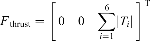
where σ is the rotor solidity, C_Lα is the lift slope coefficient, C_D is the drag coefficient, θ_b denotes the blade pitch angle, and γ_C and γ_i are the inflow factors. Finally, the total force of thrust generated by the six propellers is defined as

F_{thrust} = {[\begin{matrix} 0 & 0 & \sum_{i = 1}^{6} | T_{i} | \end{matrix}]}^{T}

Drag force

It is the opposing force to the traveling of the solid body in the air, which is resulting from the aerodynamic friction²³ and it is similar to the characteristics of the systems damping elements. This force is related to the air density and to the velocity and can be expressed by the following equation at the body’s frame: $F_{aero} = K_{T} \cdot V$ , where K_T is a diagonal matrix related to the aerodynamic friction constant by the parameter k_t.^16,20

Gravitational force

The gravity force is directed toward the center of earth during the aircraft trip in air; therefore, it is possible to describe the relation of gravity force within the frame of the aircraft body that is acting at the CG by the following equation,²⁰ where g is gravity constant

F_{grav} = m C_{n}^{b} [\begin{matrix} 0 \\ 0 \\ g \end{matrix}] = m \cdot g \cdot [\begin{matrix} sin θ \\ - sin \emptyset \cdot cos θ \\ cos \emptyset \cdot cos θ \end{matrix}]

Disturbance force

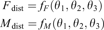
Other forces like the Coriolis force from the earth, the wind, and Euler forces are considered as a disturbance, summarized as F_dist

F_{dist} = {[\begin{matrix} F_{d 1} & F_{d 2} & F_{d 3} \end{matrix}]}^{T}

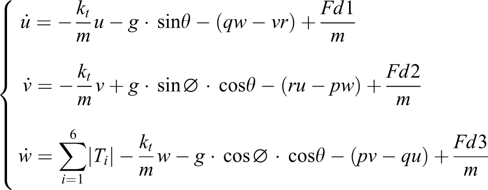
Therefore, the equations of motion that govern the translational motion based on Newton–Euler with respect to the body frame are

\begin{matrix} \sum F = F_{thrust} - F_{aero} - F_{grav} + F_{dist} \\ = m \cdot \dot{V} + Ω \times (m \cdot V) \end{matrix}

\begin{matrix} \sum F = [\begin{matrix} 0 \\ 0 \\ \sum | T_{i} | \end{matrix}] - [\begin{matrix} k_{t} u \\ k_{t} v \\ k_{t} w \end{matrix}] - m \cdot g \cdot [\begin{matrix} sin θ \\ - sin \emptyset \cdot cos θ \\ cos \emptyset \cdot cos θ \end{matrix}] + [\begin{matrix} F_{d 1} \\ F_{d 2} \\ F_{d 3} \end{matrix}] \\ = m [\begin{matrix} \dot{u} \\ \dot{v} \\ \dot{w} \end{matrix}] + m [\begin{matrix} q w - v r \\ r u - w p \\ p v - u q \end{matrix}], \end{matrix}

{\begin{matrix} \dot{u} = - \frac{k_{t}}{m} u - g \cdot sin θ - (q w - v r) + \frac{F d 1}{m} \\ \dot{v} = - \frac{k_{t}}{m} v + g \cdot sin \emptyset \cdot cos θ - (r u - p w) + \frac{F d 2}{m} \\ \dot{w} = \sum_{i = 1}^{6} | T_{i} | - \frac{k_{t}}{m} w - g \cdot cos \emptyset \cdot cos θ - (p v - q u) + \frac{F d 3}{m} \end{matrix}

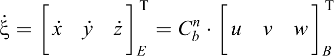
The equations of motion that governs the translational motion for the hexacopter with respect to the inertial (earth) frame are

\dot{ξ} = {[\begin{matrix} \dot{x} & \dot{y} & \dot{z} \end{matrix}]}_{E}^{T} = C_{b}^{n} \cdot {[\begin{matrix} u & v & w \end{matrix}]}_{B}^{T}

Moments analysis

The aircraft is affected by several types of moments: the thrust moment resulting from the motors, the motors inertia moment, the aerodynamic moment, and the disturbances moment. Supposing, the inertia matrix of the aircraft is J, the structure of the aircraft is symmetric, noticing that the aircraft is affected by disturbances from the robotic arm, and the controllers and the load are in the center. The moments acting around the center of the aircraft can be analyzed as follows.

Propeller moments

The M_thrust is a part of the external moments acting on the system, described by the propeller thrust $\sum_{i = 1}^{6} T_{i}$ generated by propellers, and the distance l from CG to the center of the propeller. The attitude of the vehicle in the air, that is, Euler angles $σ = {[φ θ ψ]}^{T}$ change by controlling the angular velocity of engines, that is, this moment can be expressed as: $M_{thrust} = {[\begin{matrix} M_{x} & M_{y} & M_{z} \end{matrix}]}^{T}$ , where $M_{x}, M_{y}, and M_{z}$ are the moments about the axes $X_{B}, Y_{B}, and Z_{B}$ in the body frame, noticing that the torque vectors across each other are in the same direction and the motors that are closest to each other have torque vectors in opposite directions as in Figure 3. This is the design requirement to keep the hexacopter from spinning out of control.^3,17,20 The moments generated by motors can be explained as follows as seen from Figure 3

M_{thrust} = [\begin{matrix} \frac{\sqrt{3}}{2} l (| T_{3} | - | T_{4} | - | T_{5} | + | T_{6} |) \\ \frac{1}{2} l (| T_{3} | - | T_{4} | + | T_{5} | - | T_{6} | + 2 | T_{1} | - 2 | T_{2} |) \\ ρ C_{Q} A R^{3} (ω_{1}^{2} + ω_{4}^{2} + ω_{6}^{2} - ω_{2}^{2} - ω_{3}^{2} - ω_{5}^{2}) \end{matrix}]

Figure 3.

Hexacopter architecture.

The aerodynamic moment

It is the moment resulting from the aerodynamic friction, and it affects negatively the total moment. The aerodynamic moment is expressed as: $M_{aero} = K_{R} \cdot Ω$ , where K_R is a diagonal matrix related to the rotational aerodynamic friction constant by the parameter K_r.^16,20

Disturbance moment

It is the total of the disturbances affecting the torque around the aircraft axes resulting from disturbances in the motors movement: the wind and the load in the aircraft

M_{dist} = {[\begin{matrix} M_{d 1} & M_{d 2} & M_{d 3} \end{matrix}]}^{T}

Therefore, the equations of motion that govern the rotational motion based on Newton–Euler with respect to the body frame are

\sum M = M_{thrust} - M_{aero} + M_{dist} = J \cdot \dot{Ω} + Ω \times (m \cdot Ω)

[\begin{matrix} M_{x} \\ M_{y} \\ M_{z} \end{matrix}] - [\begin{matrix} k_{r} p \\ k_{r} q \\ k_{r} r \end{matrix}] + [\begin{matrix} M_{d 1} \\ M_{d 2} \\ M_{d 3} \end{matrix}] = J [\begin{matrix} \dot{p} \\ \dot{q} \\ \dot{r} \end{matrix}] + [\begin{matrix} p \\ q \\ r \end{matrix}] \times J [\begin{matrix} p \\ q \\ r \end{matrix}]

\begin{array}{l} [\begin{matrix} \frac{\sqrt{3}}{2} l (| T_{3} | - | T_{4} | - | T_{5} | + | T_{6} |) \\ \frac{1}{2} l (| T_{3} | - | T_{4} | + | T_{5} | - | T_{6} | + 2 | T_{1} | - 2 | T_{2} |) \\ ρ C_{Q} A R^{3} (ω_{1}^{2} + ω_{4}^{2} + ω_{6}^{2} - ω_{2}^{2} - ω_{3}^{2} - ω_{5}^{2}) \end{matrix}] - [\begin{matrix} k_{r} p \\ k_{r} q \\ k_{r} r \end{matrix}] + [\begin{matrix} M_{d 1} \\ M_{d 2} \\ M_{d 3} \end{matrix}] \\ = [\begin{matrix} J_{x} \dot{p} + q r (J_{z} - J_{y}) \\ J_{y} \dot{q} + p r (J_{x} - J_{z}) \\ J_{z} \dot{r} + p q (J_{y} - J_{x}) \end{matrix}] \end{array}

\dot{p} = \frac{\sqrt{3}}{2 J_{x}} l (| T_{3} | - | T_{4} | + | T_{6} | - | T_{5} |) - \frac{k_{r}}{J_{x}} p - q r \frac{(J_{z} - J_{y})}{J_{x}} + \frac{M_{d 1}}{J_{x}}

\dot{q} = \frac{1}{2 J_{y}} l (| T_{3} | - | T_{4} | + | T_{5} | - | T_{6} | + 2 | T_{1} | - 2 | T_{2} |) - \frac{k_{r}}{J_{y}} q - p r \frac{(J_{x} - J_{z})}{J_{y}} + \frac{M_{d 2}}{J_{y}}

\dot{r} = \frac{ρ C_{Q} A R^{3}}{J_{z}} (ω_{1}^{2} + ω_{4}^{2} + ω_{6}^{2} - ω_{2}^{2} - ω_{3}^{2} - ω_{5}^{2}) - \frac{k_{r}}{J_{z}} r - p q \frac{(J_{y} - J_{x})}{J_{z}} + \frac{M_{d 3}}{J_{z}}

The equations of motion that governs the rotational motion for the hexacopter with respect to the inertial (earth) frame are

\dot{σ} = {[\begin{matrix} \dot{φ} & \dot{θ} & \dot{ψ} \end{matrix}]}_{E}^{T} = S \cdot {[\begin{matrix} p & q & r \end{matrix}]}_{B}^{T}

The suggested mathematical model as shown in the equations is characterized by nonlinearity, time variance, and close inner correlation among the system variables where any change in the input variables leads to changes in most of the output variables. Figure 4 shows a block diagram that contains the input and output variables of the dynamic model of the aircraft.

Figure 4.

Mathematical model of the hexacopter.

Control mechanism

The block diagram in Figure 4 shows the variables of the mathematical model of a multi-propeller aircraft. The control mechanism is through controlling the motors speed variables $ω_{1}, ω_{2} \dots ω_{6}$ by a defined style explained as follows:

There are three movements that describe all possible combinations of attitude: roll (rotation around the X-axis by angle φ), pitch (rotation around the Y-axis by angle θ), and yaw (rotation around the Z-axis by angle ψ). The roll control is obtained by changing the velocity of motors 3, 4, 5, and 6, and this movement is called lateral motion. Then, the pitch control is obtained by changing the velocity of all motors, resulting in the longitudinal motion. Finally, the yaw control is obtained by changing the velocity of all motors.

The change of motors speed for attitude control should be fixed and based on differential control strategy as seen in Figure 3 and equations of moments, that is, the pitch control around the Y-axis is obtained by changing the torques around this axis by increasing (T ₁, T ₃, T ₅) and decreasing another side (T ₂, T ₄, T ₆) using the following equation

ℓ \times cos 60 \times (| T_{3} | - | T_{4} | + | T_{5} | - | T_{6} |) + | T_{1} | - | T_{2} |

The roll control is obtained as follows

ℓ \times cos 30 \times (| T_{3} | - | T_{4} | - | T_{5} | + | T_{6} |)

while the yaw control is based on the torque difference between the neighboring motors

Q_{1} + Q_{4} + Q_{6} - Q_{2} - Q_{3} - Q_{5}

Altitude control is obtained by changing all motors’ velocity with a fixed change. This is based on the force equations in Z component, noticing that the thrust is equivalent to the square of the motors angular velocities. To increase the altitude, all motors velocities must be increased, and vice versa. The equation that governs the altitude is: $\sum_{i = 1}^{6} | T_{i} |$ . From the control problem based on Figure 4 and its control equations, which govern the attitude and altitude in space, the artificial vector $U = {[u_{p} u_{r} u_{y} u_{T}]}^{T}$ can be found. This simplifies the control of the system in pitch, roll, yaw, and altitude movements instead of using real motors’ velocities vector $ω = {[ω_{1} ω_{2} ω_{3} ω_{4} ω_{5} ω_{6}]}^{T}$ .¹⁷

Now we can put the equations that connect between artificial and real input vectors as follows, and Figure 5 shows the implementation

{\begin{matrix} \begin{matrix} ω_{1} = u_{T} + u_{p} + u_{y} \\ ω_{2} = u_{T} - u_{p} - u_{y} \\ ω_{3} = u_{T} + 0.5 \times u_{p} - 0.866 \times u_{r} - u_{y} \end{matrix} \\ \begin{matrix} ω_{4} = u_{T} - 0.5 \times u_{p} + 0.866 \times u_{r} + u_{y} \\ ω_{5} = u_{T} + 0.5 \times u_{p} + 0.866 \times u_{r} - u_{y} \\ ω_{6} = u_{T} - 0.5 \times u_{p} - 0.866 \times u_{r} + u_{y} \end{matrix} \end{matrix}

Figure 5.

Angular motor velocities calculation using the artificial vector.

Studying the disturbances of the arm movement in space

The block diagram in Figure 6 is the complete mathematical model of the hexacopter aircraft with the addition of disturbances block. These disturbances represent the existence of a robotic arm with a payload, which affects the overall dynamics model of the aircraft by adding moments and forces that represent noise and was defined previously in the aircraft’s equations of motion in “Aerodynamic forces and moments in axial flight” section. The disturbances that are affecting the aircraft’s CG change with time as a result of the change in the robotic arm angles in all directions, therefore making the motion equations variable with time. In this research, we suppose the representation of the arm movement with a related payload as a compound pendulum with the adoption of a mathematical procedure.^5

–8 This gives a complete and clear picture of the disturbances that are affecting the inertia moment and CG in the coordinate frame of the aircraft during its movement in the air. Since the used aircraft model is a multirotor UAV model, which is considered a solid body with a symmetric form, the parameters of the change in the disturbances functions of the motion equations can be defined according to the following general form based on the pendulum model. The shape of the aircraft was supposed approximately as a rectangle as shown in Figure 7. The pendulum motion takes place according to the angles of motion (θ₁, θ₂, θ₃) as illustrated in Figure 7, and these angles ranges are ( $0 < θ_{1} < 360, - 5 < θ_{2} < - 175, - 155 < θ_{3} < 155$ ). Assuming the weight of the payload is fixed, this leads to parameters change, the CG of the aircraft dynamics model, and the aircraft overall inertia moment, in addition to changes in the thrust resulting from the aerial motors as a result of the distance change between the CG of the aircraft dynamics model and each engine. The general form of disturbances can be expressed as follows⁹

\begin{matrix} F_{dist} = f_{F} (θ_{1}, θ_{2}, θ_{3}) \\ M_{dist} = f_{M} (θ_{1}, θ_{2}, θ_{3}) \end{matrix}

Figure 6.

Block diagram of the hexacopter dynamics system.

Figure 7.

General model of the pendulum movement disturbances.

The simplification based on the assumption that the pendulum motion occurs when the aircraft is fixed in the air in hovering position, therefore the aerodynamic effects resulting from airflow through the pendulum become neglected. In the following, the change in the overall CG and the inertia moment resulting from the pendulum motion will be studied mathematically and will be compared with the measurements resulting from the simulation depending on SolidWorks program and MATLAB program. Assuming the initial values of the pendulum angles are ( $θ_{1} = 0 °, θ_{2} = - 5 °, and θ_{3} = - 155 °$ ), and according to the physical characteristics defined in Figure 7, the pendulum parts are defined by the characteristics in Table 1, where the aircraft’s overall CG of is defined by the X _B, Y _B, Z _B coordinates. While each part of the pendulum has a local coordinate system coincide with the local CG related to that part as shown in Figure 8 in blue in comparison with the aircraft’s overall CG marked in black and white.

Table 1.

General specifications of the overall aircraft model.

M_b = 25.0 kg

M_J = 0.253 kg

M_l ₁ = 1.03 kg

M_l ₂ = 0.78 kg

M_l = 7.0 kg

Figure 8.

The workplace of the payload CG. CG: center of gravity.

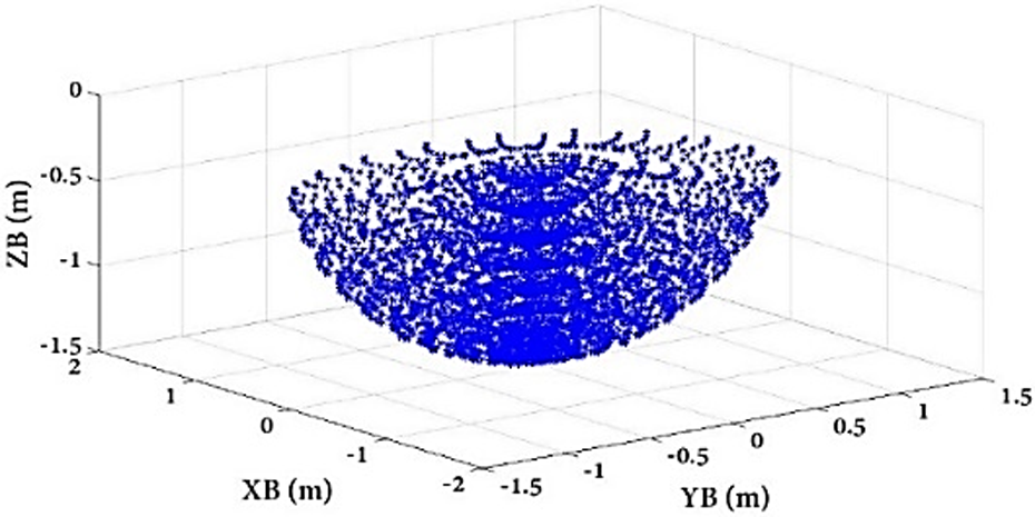
Studying the CG change

Through the study of the workspace changes of the pendulum motion in the 3-D space, the payload’s CG will draw in space a half sphere-like shape as in Figure 8. Due to these changes, the aircraft’s dynamics model CG will change accordingly through the axis of the aircraft body X _B, Y _B, Z _B, as shown in Figure 9. These changes as a whole are considered similar to half-sphere shape too. As it is noticed from the curves and as shown in Table 2, the maximum value is reached by the elements of the centers of gravity of the model. The process of studying the workspace of the movement of the centers of gravity was made using computerized simulation.

Figure 9.

The disturbances in the CG. (a) Disturbances along X _B, (b) disturbances along Y _B, (c) disturbances along Z _B and (d) disturbances in 3-D. CG: center of gravity.

Table 2.

Maximum values reached by the elements of the disturbances in the CG.

	X_B	Y_B	Z_B
Max (m)	0.2602	0.005475	0.3093
Min (m)	−0.3173	−0.2359	−0.2683

CG: center of gravity.

Studying the inertia moment

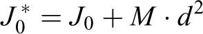
The inertia mass moment of complex shaped bodies is calculated using experimental methods, which in turn enter into many calculations within the equations of the aircraft dynamics. Here, we will adopt mathematical methods in addition to simulation in the process of estimating the moment, where the inertia moment of the overall aircraft model is given according to the formula described in the relation below, through which the mathematical study has been simplified by dividing the overall aircraft model into several parts and each part was studied separately. Where our goal is to determine the amount of inertia moment of the overall aircraft model according to the basic coordinate system X _B, Y _B, Z _B.¹⁰

J = J_{Body} + J_{Link1} + J_{Link2} + J_{Joint} + J_{Load}

where

J: Inertia moment matrix of the overall aircraft dynamics model;

J _Body: Inertia moment matrix of the aircraft body;

J _Joint: Inertia moment matrix of the joint;

J _Link1: Inertia moment matrix of the first link;

J_Link2: Inertia moment matrix of the second link; and

J_Load: Inertia moment matrix of the load.

Where the inertia moment matrix take, the general form shown in equation

J = [\begin{matrix} J_{x x} & - J_{x y} & - J_{x z} \\ - J_{y x} & J_{y y} & - J_{y z} \\ - J_{z x} & - J_{z y} & J_{z z} \end{matrix}]

The inertia for each part of the aircraft and the pendulum is studied according to several theories. Including the theory of parallel axis of Huygens-Steiner,¹⁴ which is concerned with studying the new inertia moment of the studied part relative to a new axis parallel to its axis and shifted from it by a specific distance, as in the equation below. Through our study, we will decide the inertia moment of each part of the overall model according to the coordinates system X _B, Y _B, Z _B.

J_{0}^{*} = J_{0} + M \cdot d^{2}

where $J_{0}^{*}$ is the new inertia mass moment around a new axis of rotation parallel to a local axis of rotation passing through the CG and shifted from it by a distance d. While M is the mass of the studied body, and d is the distance between the local axes of rotation of the body passing through its CG and the new axis under study. This parameter is important as it is constantly changing, because of the angles difference of the pendulum’s movement. This leads to a change in the coordinates of the new overall aircraft mass center and thus the emergence of ongoing changes in the inertia moment of the studied body with time according to the coordinate system axes of the overall aircraft dynamics model. When the coordinate system and axes between the studied part and the overall model are nonparallel, the inertia moment is then determined according to a rotation axis. This axis has different directions in angles (α, β, and γ) so that the direction of its axes at each value of the pendulum angles is parallel to the direction of the dynamics model coordinate system axis and passes through the mass center of the studied part by the mathematical relationship,^11
–13 as shown in Figure 10

J_{o} = J_{x x} α^{2} + J_{y y} β^{2} + J_{z z} γ^{2} - 2 J_{x y} α β - 2 J_{x z} α γ - 2 J_{y z} β γ

where J₀ : new inertia moment of the studied part according to new axes parallel to the output coordinates system by the angles α, β, and γ, as shown in Figure 10. While J_xx , J_yy , J_zz , J_xy , J_xz , and J_yz are the elements of the local inertia moment matrix of the studied part. The curves in Figures 11 to 16 illustrate the disturbances in the inertia moments of the aircraft overall dynamic model relative to the range of the pendulums angles change. As it is noticed from the curves and as shown in Table 3, the maximum value is reached by the elements of the inertia moments matrix of the model. Table 4 shows the errors between the calculated results based on SolidWorks program and the theoretical calculations of the values of specific samples of the pendulum angles in order to illustrate the difference between the derived values by simulation and the theoretical study.

Figure 10.

Angles of difference between the local axis of the studied body and the new axis.

Figure 11.

J_xx changes.

Figure 12.

J_yy changes.

Figure 13.

J_zz changes.

Figure 14.

J_xy changes.

Figure 15.

J_xz changes.

Figure 16.

J_yz changes.

Table 3.

Maximum values reached by the elements of the inertia moments matrix of the overall model.

	J_xx	J_yy	J_zz	J_xy	J_xz	J_yz
Max	25.21	43.06	47.31	5.872	7.179	7.44
Min	10.67	28.42	34.65	−6.24	−7.45	−7.02

Table 4.

Errors between the calculated results based on SolidWorks program and the theoretical calculations.

Moments of inertia $(kg \cdot {mm}^{2})$	No. 1	No. 2	No. 3
	θ₁° = 0	θ₁° = 72	θ₁° = 216
	θ₂° = −5	θ₂° = −158	θ₂° = −107
	θ₃° = −31	θ₃° = 46.5	θ₃° = −62
	Error (%)	Error (%)	Error (%)
J_xx	0.0000	0.2125	0.2131
J_yy	0.0026	0.1854	0.2225
J_zz	0.0017	0.2692	0.0955
J_yz	0.2319	1.6490	0.5049
J_xy	1.9312	2.0046	3.1939
J_xz	1.4129	0.3839	3.6553

These results can determine a clear vision of the disorders affecting the dynamics of the aircraft motion in space and help in implementing a model that is resistant to disturbances as much as possible in addition to designing an adaptive controller resistive to noise. Finally, we can analyze the general form of disturbances, which simulates the robotic arm motions and insert it into equations of motion specified in “Control mechanism” section. These disturbances were presented as shown in Figure 17 and were emulated based on the characteristics of the results of studies from the change of inertia moments and CG.

Figure 17.

Force and momentum disturbances resulted from the robotic arm.

We analyzed the correlation between all parameters of the hexacopter in Figure 18. The artificial input u_p is changed to 10 to control the pitch angle, and the control inputs remained fixed as follows: $u_{r} = u_{y} = 0, u_{t} = const .$ The correlation of the variables with each other makes the task of controllers design difficult, as it is noticeable in Figure 6 that the attitude variables φ, θ, and ψ are inversely related to the translational and rotational equations and therefore affect indirectly the translational and rotational motion of the aircraft. Moreover, here implementing an attitude control will affect the aircraft motion translationally and rotationally in the air. This appears obviously in the equations of motion. The curves in Figure 18 shows that controlling the pitch angle led to indirect effect on the other angles of rotational movement. The curves also show the rate of angle change, which enables us of understanding how to choose the controllers, which its response should be faster than the rate of angle change in order to avoid vibrations in the output of the aircraft. The oscillations resulted from the robotic arm connected to the hexacopter and appeared in all attitude’s variables and rates of angles because of the coupling characteristic, in addition to the nonlinearity problem that gives smooth shape to the curves affecting the accuracy of control. The scenario here is a hovering flight at an altitude of 10 m in the air. In this article, we developed a real dynamic model addressing the nonlinear, time variant, and underactuated problems because of the complexity of the dynamics. This requires precise trajectory control to stabilize the whole system and drive the hexacopter to a desired trajectory of Cartesian position, attitude and airspeed.

Figure 18.

Stability study of the hexacopter variables due to change of input u_p with the existence of disturbances.

PID controller design

In this article, we presented four linear and classical PID controllers, these controllers were adopted as it is distinguished by its ease of design and fast response, and its parameters were tuned using Ziegler Nichols algorithm²⁴ to get the best performance. The controllers speed here is considered suitable in a way that enables tracking the vibrations and changes in order to avoid the vibrations in the output of the aircraft as much as possible. The aim of these controllers is to control attitude and altitude of the vehicle at desired trajectory in space. A mathematical model of PID is described as following equation²⁴

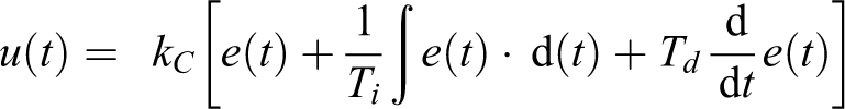
u (t) = k_{C} [e (t) + \frac{1}{T_{i}} \int e (t) \cdot d (t) + T_{d} \frac{d}{d t} e (t)]

Parameter k_c is the proportional gain, T_i is the integral time, and T_d is the derivative time. These parameters are defined, in order to get the best performance by decreasing vibrations, steady-state errors, and response time.

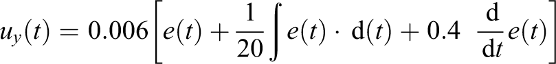
Figure 19 shows a block diagram of PIDs controlling hexacopter. The parameters of each PID used in control are defined in the following equations

u_{T} (t) = 24.19 [e (t) + \frac{1}{0.08299} \int e (t) \cdot d (t) + 0.01328 \frac{d}{d t} e (t)]

u_{p} (t) = 0.001 [e (t) + \frac{1}{6.1} \int e (t) \cdot d (t) + 0.1 \frac{d}{d t} e (t)]

u_{r} (t) = - 0.00103 [e (t) + \frac{1}{6.3} \int e (t) \cdot d (t) + 0.04073 \frac{d}{d t} e (t)]

u_{y} (t) = 0.006 [e (t) + \frac{1}{20} \int e (t) \cdot d (t) + 0.4 \frac{d}{d t} e (t)]

Figure 19.

The block diagram of a PID controller connected to the hexacopter model. PID: proportion, integral, and derivative.

To control a hexacopter an application was conducted by LabVIEW using Runge–Kutta 2 method with a fixed step of 0.05 s. Four PID controllers were implemented to stabilize the altitude and attitude as shown in Figures 20 to 24. The curves show the control signal and the fast response of the controllers with the existence of disturbances, which emulates the existence of an arm in a non-laboratory environment. These controllers avoid the occurrence of vibrations in the output variables of the flying object as possible. The tuning process has been achieved after many experimental trials. Our scenario is the hovering flight at the altitude of multilevels in the air. Future work focuses on developing a precise trajectory control by using robust techniques to stabilize the whole system and drive the hexacopter to the desired trajectory of Cartesian position, attitude, and airspeed. The system’s parameters, which has been used in the simulation model, are listed in Table 5. Correlations were analyzed for all parameters of motion equations.

Figure 20.

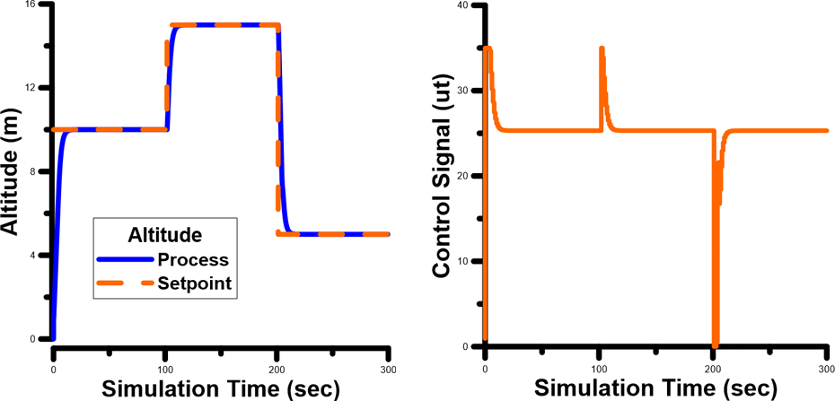
Stability response of altitude and control signal.

Figure 21.

Stability response of pitch angle and control signal.

Figure 22.

Stability response of roll angle and control signal.

Figure 23.

Stability response of yaw angle and control signal.

Figure 24.

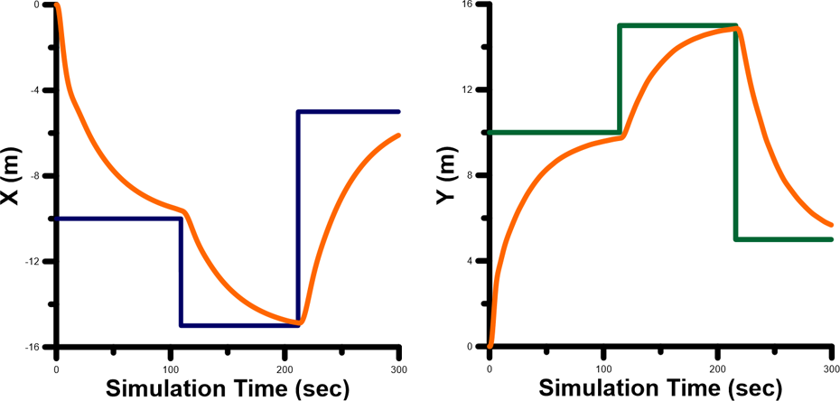
Stability response of X and Y coordinate systems.

Table 5.

Parameters used in the simulation.

m = 4 kg	g = 9.806 m/s²	l = 0.5 m
J_x, J_y = 3.8e⁻⁴ kg·m·s²/rad	R =0.15 m	k_t = 4.8e⁻³ kg·s/m
J_z = 7.1e⁻⁴ kg·m·s²/rad	A = 0.071 m²	k_r = 6.4e⁻⁵ kg·m·s/rad
C_T = 0.01458	C_Q = 1.037e⁻³	ρ = 1.293 kg/m³

Stability analysis

Curves in Figures 20 to 24 show the control signal and the quick response of the controllers with the existences of disturbances, which emulate the existence of an arm in non-laboratory environment. These controllers avoid the occurrence of vibrations in the output variables of the flying object as possible. Taking into consideration an analytic study of the controller’s stability based on studying the unity response with several different levels of altitude and attitude according to Table 6, we find that these controllers are suitable but not ideal and require development in order to get optimal results. Currently developing the controllers is going on in order to get robust stability through including nonlinear techniques and artificial intelligence.

Table 6.

Stability response of PID controllers.

PID controller	Response time (s)	Steady-state error
Altitude	22.5	−0.0911 (m)
Pitch	8.15	0.01955 (°)
Roll	5.72	0.0941 (°)
Yaw	5.58	0.00173 (°)

PID: proportion, integral, and derivative.

Conclusions

A real and complex dynamic model was considered, which addresses the nonlinearity, time variance, underactuation, and disturbance. This article gives a complete discussion of the determination of the moments of inertia by simplified pendulum method, in addition to taking into consideration the effects of mass distributions and CG change. These disturbances were inserted into the equations of motions, which also simulate a robotic arm motion while the aircraft model is flying in the sky. An application was conducted using SolidWorks and LabVIEW using Runge–Kutta 2 method. Correlations were analyzed for all parameters of motion equations. Four PID controllers were implemented to stabilize the altitude and attitude. These controllers’ parameters were tuned using Ziegler Nichols algorithm to get the best performance and avoid the occurrence of vibrations in the output variables of the flying object as possible. These controllers are suitable but not ideal and require improvement in order to get optimal results. Future work focuses on developing a precise trajectory control by using robust techniques to stabilize the whole system and leads the hexacopter to the desired trajectory of Cartesian position, attitude, and airspeed.

Footnotes

Declaration of conflicting interests

The author(s) declared no potential conflicts of interest with respect to the research, authorship, and/or publication of this article.

Funding

The author(s) disclosed receipt of the following financial support for the research, authorship and/or publication of this article: The contribution is sponsored by VEGA MŠ SR No 1/0367/15 prepared project, “Research and development of a new autonomous system for checking a trajectory of a robot” This publication is the result of implementation of the project: “UNIVERSITY SCIENTIFIC PARK: CAMPUS MTF STU - CAMBO” (ITMS: 26220220179) supported by the Research & Development Operational Program funded by the EFRR.

References

Schmidt

. Simulation and control of a quadrotor unmanned aerial vehicle. Master’s Theses, Lexington, USA, University of Kentucky U Knowledge, 2011.

Xin

Yannian

. Control design and analysis for underactuated robotic systems. Okayama: Okayama University Japan; London: Springer London, 2014. ISBN: 978-1-4471-6251-3.

Lucia

Tipaldi

GD,

Burgard

. Attitude stabilization of an aerial manipulator using a quaternion-based back-stepping approach. In: IEEE-2015 European Conference, University of Freiburg, Germany, 2–4 September 2015.

Alvarez-Munoz

Marchand

Guerrero-Castellanos

. Nonlinear control of a nano-hexacopter carrying a manipulator arm. In: IEEE-2015/RSJ International Conference on Intelligent Robots and Systems (IROS), Congress Center Hamburg, Germany, 28 September–2 October 2015.

Soule

Miller

. The experimental determination of the moments of inertia of airplanes. Report for National Advisory Committee for Aeronautics (NACA). Report no. 467, 01 January 1934. Washington, USA.

Gracey

. The experimental determination of the moments of inertia of airplanes by a simplified compound-pendulum method. Report for National Advisory Committee for Aeronautics (NACA). Report no. 1629, 01 June 1948. Washington, USA.

Pobedonoszeff

. An experimental method of determination of the moments of inertia of aeroplanes. Report no. 20l, 1935. Trans. CAHI, Moscow.

Miller

. An accurate method of measuring the moments of inertia of airplanes. Report for National Advisory Committee for Aeronautics (NACA). Report no. 351, 01 October 1930. Washington, USA.

Mathews

Walker

. Mathematical methods of physics, 2nd ed. New York: WA Benjamin, 1970.

10.

Malvestuto

Gale

. Formulas for additional mass corrections to the moments of inertia of airplanes. Report for National Advisory Committee for Aeronautics (NACA). Report no. 1187, 01 February 1947. Washington, USA.

11.

Favorin

. Моменты Инерции Тел: Справочник, 2nd ed. Moscow: Mashinostroenie, 1977.

12.

Arfken

Weber

Harris

. Mathematical methods for physicists: a comprehensive guide. Waltham, Massachusetts, USA: Academic press, 2011.

13.

Gernet

Ratobyl’skii

. Opredelenie Momentov Inertsii. Moscow: Mashinostroenie, 1969, p. 247.

14.

Kane

Levinson

. Dynamics, theory and applications (McGraw Hill Series in Mechanical Engineering), 1st ed. New York, USA: Mcgraw-Hill College, 1985.

15.

Alvarez-Munoz

Marchand

Guerrero-Castellanos

. Improving control of quadrotors carrying a manipulator arm. In: XVI Congreso Latinoamericano de Control Automatico (CLCA 2014), Mexico, 14–17 October 2014, p. 6.

16.

Sanca

Laura

Cerqueira

. Dynamic modeling with nonlinear inputs and backstepping control for a hexa-rotor micro-aerial vehicle. In: 2010 Latin American Robotics Symposium and Intelligent Robotics Meeting (LARS), Sao Bernardo do Campo, Brazil, 23–28 October 2010, pp. 36–42.

17.

Moussid

Sayouti

Medromi

. Dynamic modeling and control of a hexa-rotor using linear and nonlinear methods. Int J Appl Inform Syst (IJAIS) 2015; 05: 9–17.

18.

Moussid

Idalene

Sayouti

. Autonomous hexa-rotor aerial dynamic modeling and a review of control algorithms. Int Res J Eng Technol (IRJET) 2015; 05: 1197–1204.

19.

Julián

Colorado

. Towards miniature MAV autonomous flight: a modeling and control approach. Master thesis, Science in Robotics and Automation, Technical University of Madrid, Spain, 4 2009.

20.

Magnussen

Skjonhaug

. Modeling, design and experimental study for a quadcopter system construction. Master Thesis, Faculty of technology and science/University of Agder-Kristiansand S, Norway, 2011.

21.

Artale

Milazzo

CLR,

Ricciardello

. Mathematical modeling of hexa-copter. Appl Math Sci Kore Univ Enna Italy 2013; 7(97): 4805–4811.

22.

Chovancová

Fico

Chovanec

. Mathematical modeling and parameter identification of quadrotor (a survey). Proc Eng 2014; 96: 172–181.

23.

Sjoholm

Biel

Automatic control of a quadrotor in the smart building. Master Thesis, School of Engineering Sciences/KTH Royal Institute of Technology, Stockholm, Sweden, 2014.

24.

Astrom

Murray

. Feedback systems, vol 2(11b). Princeton, New Jersey, USA: Princeton University Press, 2012. ISBN: 978-0691135762.