
Abstract
Hydraulic actuated quadruped robot similar to BigDog has two primary performance requirements, load capacity and walking speed, so that it is necessary to balance joint torque and joint velocity when designing the dimension of single leg and controlling its motion. On the one hand, because there are three joints per leg on sagittal plane, it is necessary to firstly optimize the distribution of torque and angular velocity of every joint on the basis of their different requirements. On the other hand, because the performance of hydraulic actuator is limited, it is significant to keep the joint torque and angular velocity in actuator physical limitations. Therefore, it is essential to balance the joint torque and angular velocity which have negative correlation under the condition of constant power of the hydraulic actuator. The main purpose of this article is to optimize the distribution of joint torques and velocity of a redundant single leg with joint physical limitations. Firstly, a modified optimization criterion combining joint torques with angular velocity that takes both support phase and flight phase into account is proposed, and then the modified optimization criterion is converted into a normal quadratic programming problem. A kind of recurrent neural network is used to solve the quadratic program problem. This method avoids tremendous matrix inversion and fits for time-varying system. The achieved optimized distribution of joint torques and velocity is useful for aiding mechanical design and the following motion control. Simulation results presented in this article confirm the efficiency of this optimization algorithm.
Keywords
Introduction
The quadruped robot prototype is shown in Figure 1, whose structure and configuration could be described as follows: four symmetrical legs, four revolute joints and hydraulic actuators per leg, and a torso hinged by legs and equipped with computer, controller, and sensors. Since the robot’s motion such as walking, running, and hopping is produced mainly by legs’ movement, mechanism dimension design of the legs and control of the single leg are crucial for control of the whole robot. Figure 2 shows the single-leg design drawing in which there are four joints and actuators, three of which are in the sagittal plane and the rest one is in the lateral plane. The red lines in Figure 2 are the most important dimensions. As moment arms of actuating forces, they decide not only the maximum joint torques but also the maximum joint angular velocity on condition that the actuating force and velocity of the hydraulic actuator are limited. The design process as shown in Figure 3 presents firstly, optimizing the joint angular velocity and torques based on performance requirements, secondly, choosing proper mechanism dimensions that satisfy actuator performance limitations, and at last, testing and verifying its effectiveness according to simulation and experiment.
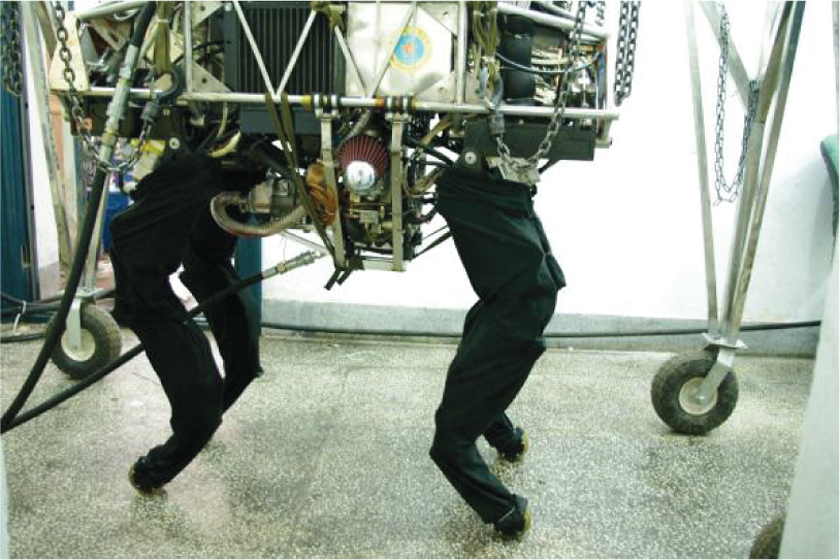
The quadruped robot.
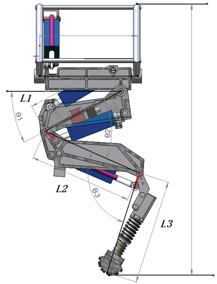
The single-leg model.

The design process of single-leg dimension.
In this article, one part of the design process shown in Figure 3, that is, single-leg optimization, is discussed. The main task of single-leg optimization is to optimize the inverse kinematics of the redundant single leg on the basis of performance requirements and distribute joint torques and angular velocity according to different requirements of every joint with joint physical limitations. There are two kinds of methods to solve inverse kinematics problem of redundant robots, that is, analytical method and optimization method. For a redundant robot, analytical solution of its inverse kinematics is generally expressed as a function of some variable parameters, such as joint angles 1,2 or the included angle between the robot and the reference plane. 3,4 Setting constraints is also used to solve the inverse kinematics problem. 5 If the number of constraints equals to the redundant degrees of freedom, analytical solutions of inverse kinematics could be acquired.
Because of the high nonlinearity and strong coupling, solving the inverse kinematics problem of redundant robot is tedious. Sometimes only those redundant robots with specific structure have analytical inverse kinematics. Moreover, analytical solution usually neglects the motion performance of the redundant robot and the advantages of redundant degrees of freedom. Resolving the redundant degrees of freedom properly will contribute to avoiding obstacles, 6 joint physical limits, 7 and singularities. 8 The redundant degrees of freedom could also be utilized to optimize various motion performance criteria. 9 –12 On that account, a number of researchers optimized the inverse kinematics of the redundant robot based on various performance criteria. The problems without inequality constraints have closed-form analytical solutions, while those with inequality constraints could obtain numerical solution by iterative method. One conventional solution is pseudo-inverse-type formulation. 13,14 Szkodny and Legowski 15 and Nie et al. 16 used interpolation method to solve inverse kinematics problem, but this method is subjected to heavy computation and accumulative error. Kokurin, 17 Liu et al., 18 and Jin et al. 19 used gradient projection method to solve inverse kinematics problem, but the definition of the gradient function decides that the results don’t always contain the optimal solution in essence. Other methods are also used to solve inverse kinematics problem, such as online learning algorithm, 20 quadratic programming, 21 quaternion method, 22 genetic algorithm, 23 and neural networks. 24 Thereinto, quadratic programming becomes a preferable algorithm because of its simpleness and real-time capability. The most widely adopted optimization criterion is the minimum velocity norm (MVN), that is, the optimization process results in minimum sum of squares of joint velocity. Its mathematical tractability makes online computation easy, while it neglects dynamical performance completely. 25 On the contrary, the optimization criterion, minimum torque norm (MTN), is also used in quadratic programming to minimize the sum of squares of joint torques. However, the joint-torque minimization scheme may lead to system instability, divergence from the desired values, and even sudden changes.
To solve or decrease the negative effects of aforementioned problems, Ma 26 proposed a balancing technique, that is, an optimization criterion consisting of joint-torque minimization and joint-velocity minimization. However, Ma made use of the conventional pseudo-inverse-type formulation, which has high computation complexity and risk of singularity. Unlike the pseudo-inverse-type formulation, Zhang et al. 27 proposed and investigated a constrained balancing minimization scheme (i.e. different-level simultaneous minimization scheme) to stabilize optimal motions of redundant manipulators. The proposed minimization scheme combines the minimum two-norm joint-velocity and joint-torque solutions via two weighting factors and incorporates the avoidance feature of joint physical limits as well. Note that such a different-level simultaneous minimization scheme is finally transformed into a quadratic program (QP) at the joint-acceleration level and solved by using a primal–dual neural network (PDNN) based on linear variational inequality (LVI). 28 –30
Differing from the robot manipulators, for legged robots, there are support phase and flight phase when they are walking. A single leg of legged robots not only supports the body in support phase but also swings forward to the foot placement point alternatively. On the basis of different task requirements, a single leg is demanded to provide sufficient support force meaning sufficient joint torques in support phase and provide sufficient foot velocity meaning sufficient joint velocity and lesser joint torques in flight phase (swing phase). On that account, it is needed to design an optimization criterion different from that proposed by Ma 26 and Zhang et al. 27 On the other hand, the optimization techniques used by Zhang et al., 27 that is, the PDNN based on LVI, have the advantages of briefness and tractability, so we adopt this algorithm in this article.
The rest of this article is organized into four sections. Firstly, the scheme formulation of the different-level simultaneous minimization scheme taking both support phase and flight phase into consideration is proposed for a single leg of quadruped robot with physical constraints. Then the scheme is reformulated into a QP problem similar to the process method in the literature. 27 And the QP problem is solved by using the LVI-based primal–dual neural network (LVI-PDNN) and its closed-loop LVI-based primal–dual neural network (CLVI-PDNN). Secondly, we propose a new kind of method named Mid-Value CLVI-PDNN based on LVI-PDNN in order to overcome its drawbacks. Thirdly, we illustrate the computer simulation results including observations and comparisons, which demonstrate the efficiency of the proposed method. At last, we conclude this article with final remarks.
The optimization criterion and QP formulation
Before presenting the optimization criterion, it is necessary to describe the single-leg system briefly. The kinematics of the single leg in the sagittal plane could be described as a nonlinear equation

in which

in which

in which

The dynamics of the single leg in the sagittal plane could be described as

where H(θ) denotes inertia matrix of the single leg,
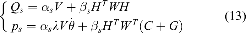
As mentioned in the previous section, an invariant optimization criterion in all time doesn’t fit for legged robots. Because of its unique characteristic, a piecewise optimization criterion corresponding to different phases is reasonable. The modified optimization problem combining of minimum two-norm joint velocity and torque is formulated as

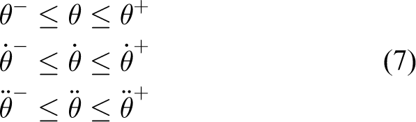
subjected to equations (4) and (5), and the joint physical limitations of the mechanism such as
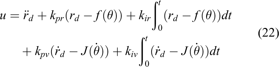
α and β are weight factors with subscripts s and f meaning support phase and flight phase. Their values fall in the interval [0 1] satisfying
Just like the conversion method proposed by Zhang et al.,
27
the optimization criterion in equation (6) could be converted into a standard QP programming. Because

where λ is a constant that determines the convergent rate. The equation

therefore, minimizing
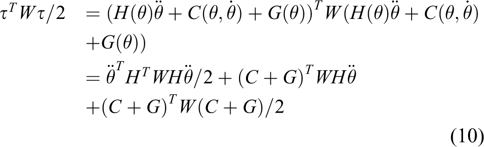
Similarly, it could be achieved that minimizing τ
T
Wτ/2 is equivalent to minimizing
According to the analysis above, the optimization problem described by equations (4)–(7) with different levels of angular velocity and joint torques scheme could be converted into a standard QP problem as below

with constraints

where

The QP problem could be further converted to an LVI problem equivalent to a piecewise linear system as follows

where PΩ(⋅) is a piecewise-linear projection operator as shown in Figure 4. y denotes the primal–dual decision variable vector. qs and qf denote the coefficient vectors. Matrices Ms and Mf are the augmented matrices with J


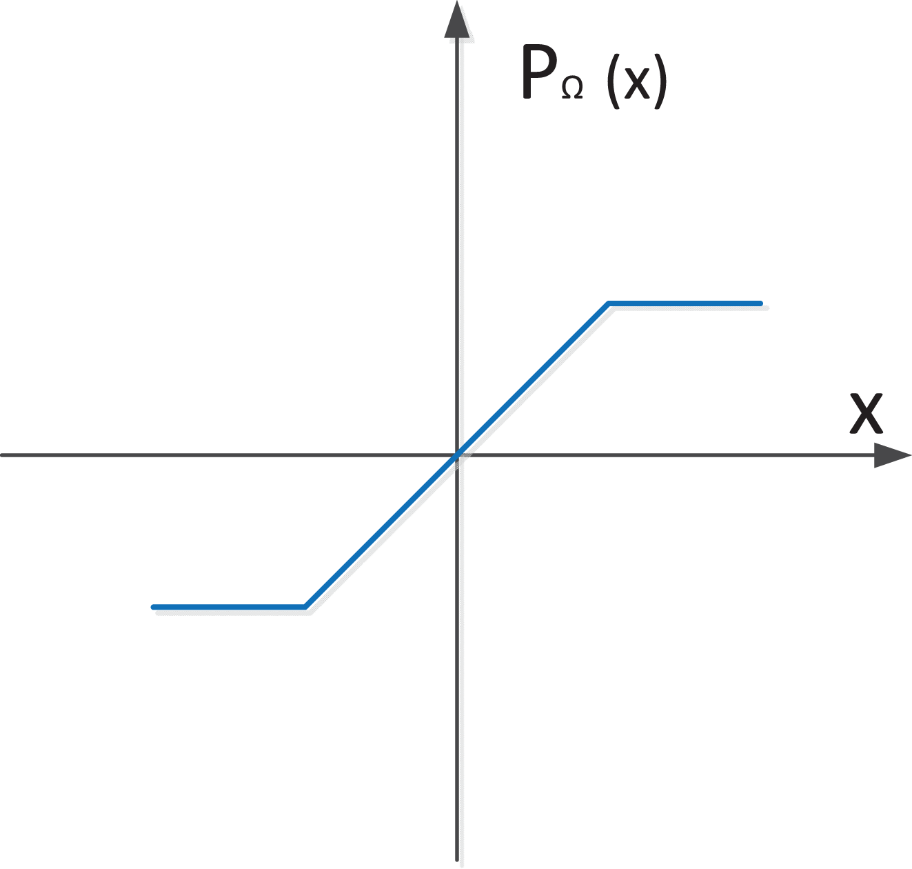
Piecewise-linear projection operator PΩ(⋅).
where x means the dual decision variable vector relevant to the equality constraints. The process of converting the constrained QP problem described in equations (11) and (12) to an equivalent LVI problem, then converting the LVI problem to an equivalent piecewise linear equation like equation (15), is no longer detailed in this article and one could refer to the literature 30 for details.
Zhang et al. 27 used LVI-PDNN to solve the QP problem. The dynamic equation of the neural network is reformulated following Zhang as below

where γ is a constant that could scale the convergence rate of the neural network system and should be selected as large as possible. The block diagram of the LVI-PDNN is shown in Figure 5. As aforementioned, since Zhang et al. solved the optimization problem for a manipulator robot, the problem of different phases of the robot needn’t be considered, while our quadruped robot has support phase and flight phase when moving forward.

Block diagram of LVI-PDNN. LVI-PDNN: LVI-based primal–dual neural network; LVI: linear variational inequality.
It is worth pointing out that the LVI-PDNN treats the QP optimization problem as a control problem and its structure is open loop actually. Consequently, the open-loop algorithm would probably be effective in some circumstances such as the manipulator robots, but it indeed loses efficacy when processing the optimization problem of the quadruped robot because it leads to divergent results. The divergency is perhaps caused by modeling uncertainty and switch between support phase and flight phase. Naturally, we try to adopt a closed form to avoid diverging. The original LVI-PDNN could be transformed to CLVI-PDNN that is shown in Figure 6. The part in the blue dotted line is the original LVI-PDNN. The part outside of the blue dotted line forms a closed loop, and the feedback could be achieved according to equations (1) and (2) as below
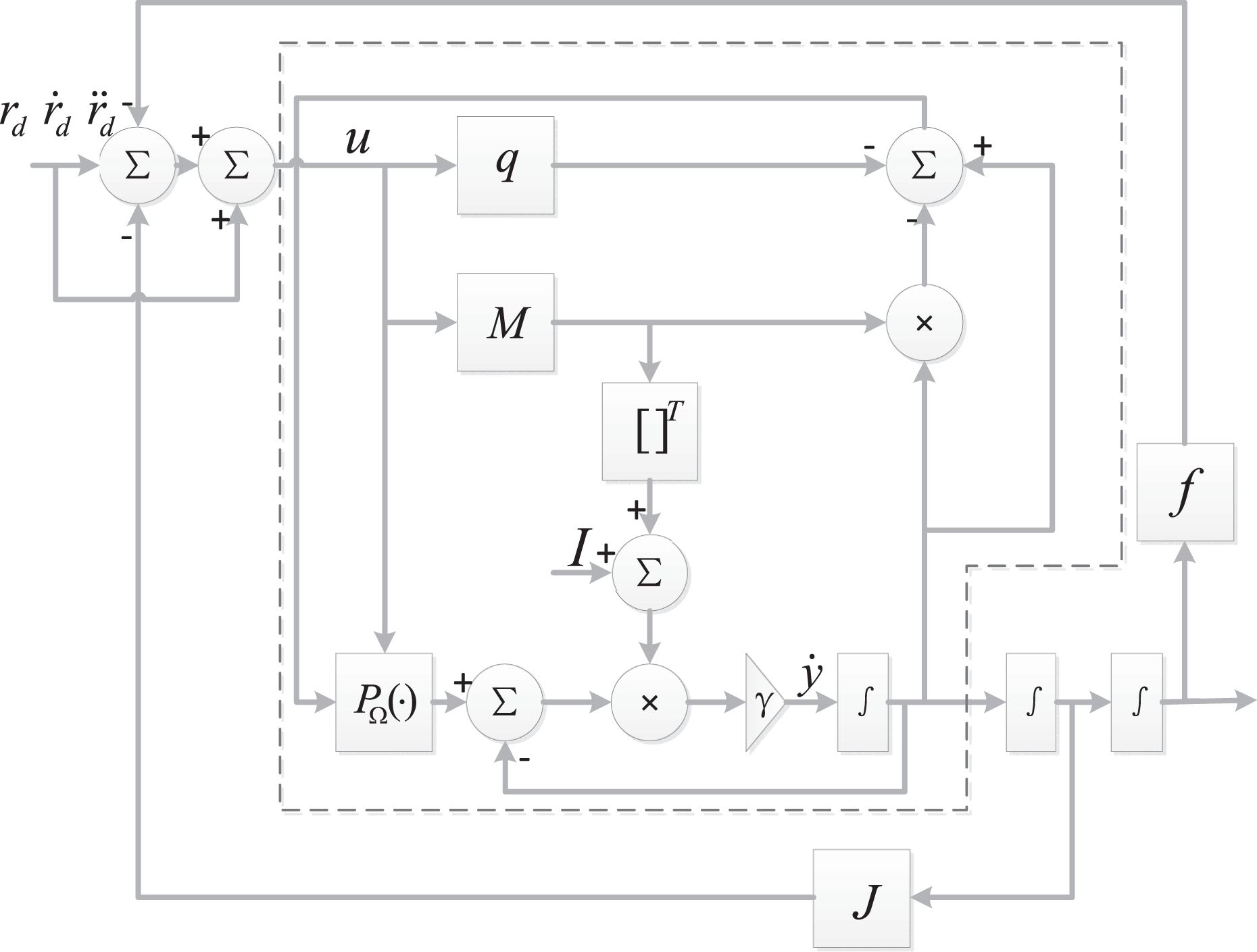
Block diagram of CLVI-PDNN. CLVI-PDNN: closed-loop LVI-based primal–dual neural network; LVI: linear variational inequality.
where u means the input of LVI-PDNN. rd,
Mid-value CLVI-PDNN optimization
As described in the previous section, the joint angles and velocity integrated from output of the QP solver, that is, joint angle acceleration, are introduced to the input as feedback for ensuring exponential convergency of the algorithm. However, the output of the CLVI-PDNN QP solver (joint angles) without integral threshold constructs undesired unreasonable configuration of the single leg as shown in Figure 7. Figure 7 shows that θ1 is expected to be an acute angle, while the output is an obtuse angle. Similarly, θ2 is expected to be an inferior angle but the output is a reflex angle. The result violates the joint physical constraints actually. We tried to achieve the desired valid configuration through tuning parameters of the CLVI-PDNN QP solver listed in Table 2. Unfortunately, it seems to be useless even though we tried our best. Another method that is naturally picked up is to set integral threshold as listed in Table 4. The joint physical constraints are rigid constraints that need to be satisfied prior. Consequently, it may weaken some soft constraints such as equality constraints. The results that are shown in the next section demonstrate the characteristic of this method, that is, the tremendous difference between the desired and actual trajectory of the foot in operation space.

The reasonable and undesirable leg configuration.
To prevent from violating the joint physical constraints, we define a slack variable ε = θ − θd, in which θd means a desired joint configuration of the single leg within the joint limitations listed in Table 4. A simple feedback control method could maintain stability of ε as below

where θ0 is the initial values of joint angles and kp is a positive coefficient matrix. The value of θd could be selected close to the mid-value of the motion range of the joints to avoid collision with the joint physical limitations. The block diagram of this algorithm is depicted in Figure 8. Because the selection of θd is close to the mid-value of joint motion range, this algorithm is named Mid-Value CLVI-PDNN.

The block diagram of Mid-Value CLVI-PDNN. CLVI-PDNN: closed-loop LVI-based primal–dual neural network; LVI: linear variational inequality.
Actually, we attempt to balance between the equality constrains and inequality constrains. That means on the one hand, the output of the QP solver doesn’t exceed the physical limitations ensuring a feasible solution in spite of non-optimal value. On the other hand, the difference between the desired and the optimized trajectory in operation space decreases as much as possible although violating the equality constrains to some extent. Nonetheless, the simulation results presented in the next section will show that the error of trajectory in operation space is rather negligible with respect to the size of the single leg. In a sense, the Mid-Value CLVI-PDNN QP solver and its output would be applicable in many scenarios that don’t require high accuracy such as legged robot walking in the field.
Although we insert a slack variable into the CLVI-PDNN QP solver, ε won’t damage the stability of the new QP solver because of its closed form described in equation (23). This characteristic could also be made out according to the simulation results in the next section. For some circumstances, such as high dimensions of the augmented matrix Ms and Mf, restricted performance of the onboard controller or computer, the discrete form of the QP solver proposed in this article may be more applicable for real-time control. We will deduce the discrete form of Mid-Value CLVI-PDNN and analyze its characteristics in another paper.
We apply the algorithm proposed in this article to a single leg as shown in Figure 2 and some simulation results will be presented in the next section.
Simulation
We operate the QP solver proposed in this article in Matlab to solve the two-norm optimization problem. It is supposed that a quadruped robot moves along a straight line on horizontal direction using trotting gait, and the single leg alternates between support phase and flight phase. Since two legs support the body all the time when the quadruped robot trots forward, every leg bears nearly half of the whole mass. The single leg has three joints in the sagittal plane, that is, hip joint, knee joint, and ankle joint. The physical parameters of the single leg are listed in Table 1, where M denotes the mass of the body. M1, M2, and M3 denote the masses of the three links of the single leg. L1, L2, and L3 denote the lengths of the three links.
Physical parameters of the single leg.
The parameters of the CLVI-PDNN are listed in Table 2. The parameters of the trotting gait are listed in Table 3. h denotes the height of the hip. hapex denotes the maximum height of the foot in flight phase. v is the desired velocity of the body. T is the gait cycle time interval. g is the gravitational acceleration. The body moves at a constant speed in sagittal plane with constant height h. Additionally, in flight phase, the trajectory of the foot on the horizontal direction is achieved by cubic spline interpolation, while the foot moves along sine curve on the vertical direction. The limitations of angular acceleration, angular velocity, and angles are listed in Table 4.
Parameters of the CLVI-PDNN.

CLVI-PDNN: closed-loop LVI-based primal–dual neural network; LVI: linear variational inequality.
Parameters of the trotting gait.
Physical limitations of joint.

The weight matrices V and W are used to distinguish different joints about joint torques and velocity, and they are set as
The joint angles integrated merely from the output of LVI-PDNN solver proposed by Zhang et al. 27 actually diverge in our simulation. The results obtained from the CLVI-PDNN QP solver without integral threshold are depicted in Figures 9 to 11. The results demonstrate that although the trajectory in operation space could match the desired value perfectly, the joint angles exceed its physical limitations. And that the joint angles could not return into the physical limitations no matter how to tune the parameters.

The results of unlimited CLVI-PDNN with

The results of unlimited CLVI-PDNN with

The results of unlimited CLVI-PDNN with
The results optimized by CLVI-PDNN QP solver with integral threshold to prevent joint angles from exceeding the physical limitations are shown in Figures 12 to 14. These results demonstrate severe distortion of the output of this QP solver compared to the desired trajectory in operation space, especially the enormous position error in horizontal direction. Although abiding by the CLVI-PDNN QP solver and restricted into the physical constraints, the results would lead to divergence between the optimized values and the desired values.
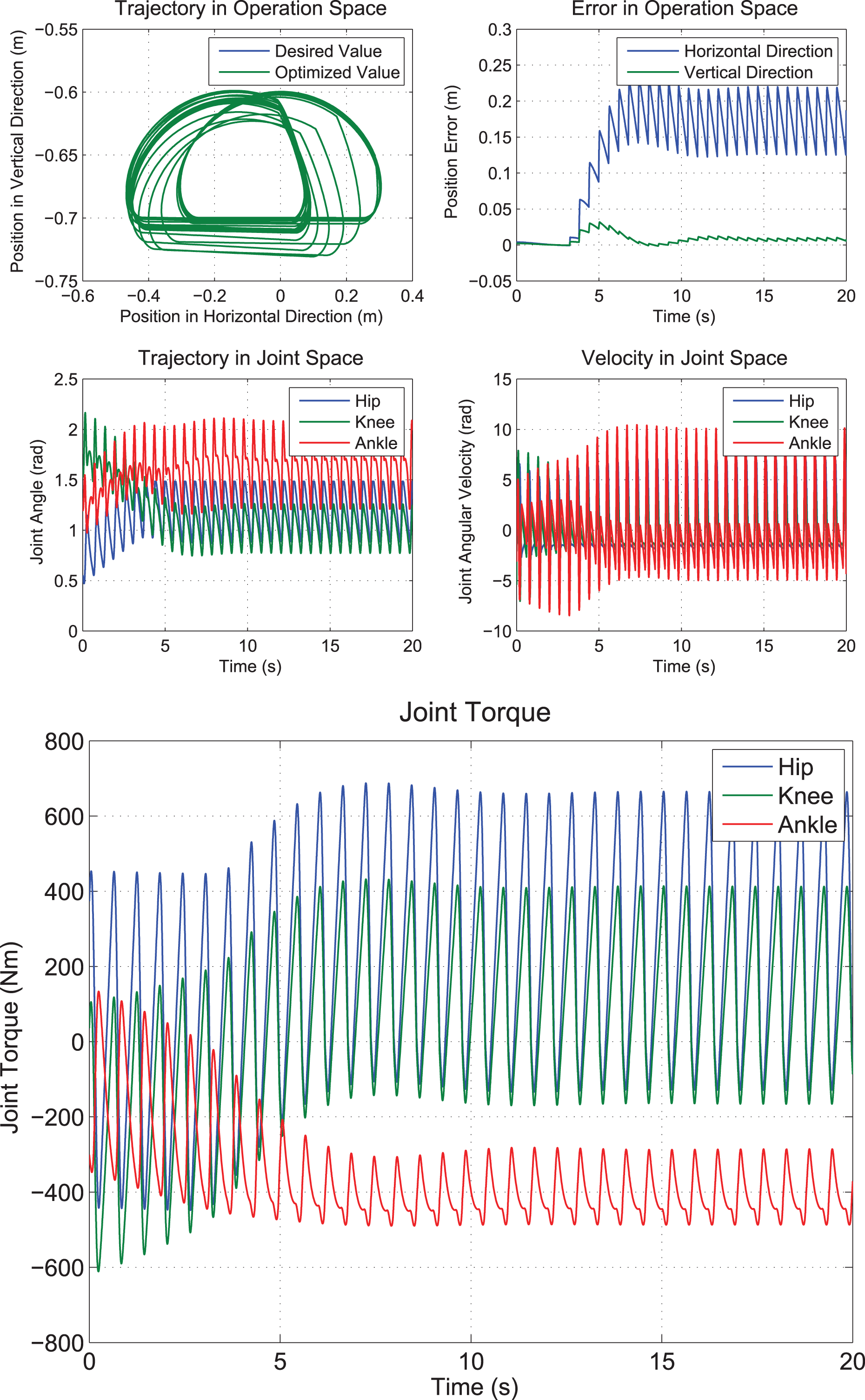
The results of limited CLVI-PDNN with

The results of limited CLVI-PDNN with

The results of limited CLVI-PDNN with
To solve the problems that emerge in the LVI-PDNN and CLVI-PDNN QP solvers, we propose the Mid-Value CLVI-PDNN QP solver in this article, whose results are illustrated in Figures 15 to 18. The results shown in Figures 15 to 17 are acquired with

The results of Mid-Value CLVI-PDNN with

The results of Mid-Value CLVI-PDNN with

The results of Mid-Value CLVI-PDNN with

The results of Mid-Value CLVI-PDNN with
Nevertheless, the Mid-Value CLVI-PDNN QP solver brings about several problems. One of the problems is that tuning the parameters such as V, W and αs, αf has less effect on the joint torques. In other words, the joint torques don’t reflect the desired variation tendency. The reason may be that the results are not the intuitional optimal solution relevant to the optimization criterion in equation (6), once inserting the slack variable ε = θ − θd. But when changing the value of θd, the joint torques change obviously as shown in Figure 18.
The simulation results illustrated in Figures 9 to 18 are summarized in Table 5. The parameters and performance of the QP solvers used in this article are all collected in the table. Unlimited CLVI-PDNN means the CLVI-PDNN QP solver without integral threshold, while Limited CLVI-PDNN means the CLVI-PDNN QP solver with integral threshold. The columns corresponding to V and W are the diagonal elements. The columns corresponding to ωmax and τmax mean the maximum joint angular velocity and maximum joint torque, where h, k, a in brackets denote hip joint, knee joint, and ankle joint, respectively. The columns corresponding to eh and ev denote the position error between the optimized value and the desired value in the horizontal and vertical directions, respectively. The order of magnitude of the position error is presented in the table. The last column indicates whether the optimized results violate the joint physical limitations.
Summary of the simulation results.

CLVI-PDNN: closed-loop LVI-based primal–dual neural network; LVI: linear variational inequality; h: hip joint; k: knee joint; a: ankle joint.
Conclusion
To solve the inverse kinematics of the redundant single leg of the quadruped robot, we propose a modified optimization criterion taking both support phase and flight phase of legged robot into account. Then the Mid-Value CLVI-PDNN QP solver is developed on the basis of LVI-PDNN proposed by Zhang et al. 27 The results illustrated in the previous section demonstrate efficiency of the Mid-Value CLVI-PDNN QP solver. However, we could conclude from the results that the Mid-Value CLVI-PDNN compromises between the LVI-PDNN and CLVI-PDNN, that is, acquiring proper joint angles with reasonable joint angular velocity at the cost of precision of the optimized trajectory compared to the desired motion trajectory in operation space. It is exactly what is neglected in the method proposed by Zhang et al., 27 but we do fail to get touch with the author to consult some better solutions or recommendations. Ever so matter-of-factly, the Mid-Value CLVI-PDNN doesn’t provide intuitional optimal solution relevant to the optimization criterion in equation (6) but a simple feasible solution. In addition, how to select the value of θd is of great importance to acquire valid output of this QP solver.
In application, the optimized solution is not only used for mechanism design but also the following motion control of the single leg further. Actually, the Mid-Value CLVI-PDNN QP solver could be used for other redundant robot leg or manipulator. And we will utilize this algorithm to solve the contact force distribution of the quadruped robot in the future.
Footnotes
Declaration of conflicting interests
The author(s) declared no potential conflicts of interest with respect to the research, authorship, and/or publication of this article.
Funding
The author(s) disclosed receipt of the following financial support for the research, authorship, and/or publication of this article: This research received grant from National Hi-tech Research and Development Program of China (grant no. 2015AA042202) and National Nature Science Foundation of China (grant no. 61473304).