Sage Journals: Discover world-class research

Abstract

This article presents an implementation of an adaptive control architecture, which provides the combined advantages of better dynamic performance compared to other conventional industrial controllers, and the use of widely available hardware in process industry. Adaptive control architecture uses proportional–integral action and dynamic computation of the controller’s gains (self-tuning regulator), to maintain performance specifications, even in the presence of parametric disturbances. This architecture offers advantages over other advanced embedded control systems implemented on industrial programmable logic controllers and other hardware platforms. Implementation of controllers on industrial hardware platforms is possible through the Object Linking and Embedding (OLE) for process control communication standard. The implementation for an adaptive controller here proposed was evaluated through experiments using first-order and overdamped second-order systems emulated by hardware-in-the-loop, with a programmable automation controller. Performance of the adaptive controllers was compared to that of conventional proportional–integral controllers, and effectiveness of the former over the latter was demonstrated through the experiments carried out.

Keywords

Self-tuning regulators PI controller recursive least squares programmable logic controllers OPC hardware-in-the-loop

Introduction

In industry applications, more than 95% of the used control loops are of the proportional–integral–derivative (PID) type.¹ PID controllers were introduced in industrial processes by the end of the 1930s.² The use of these controllers is extensive due to the following main advantages:

Their good performance in a wide variety of applications within industrial processes and manufacturing automation.

The fact that commercial PID controllers are relatively inexpensive.

PID controllers can be tuned using heuristic methods, although their performance is better when they are tuned with an analytic tool.

The work of existing technological platforms is to aid in the implementation of PID controllers, thus the adoption of different control strategies can represent technical and economic difficulties.

The use of PID controllers in industrial processes and manufacturing is comparatively less effective than using other controllers systems in the presence of nonlinear dynamics, disturbances, and parametric uncertainties (in sensors, in actuators, and in the process itself). That is to say, when it comes to industrial processes, performance of PID controllers can be unsatisfactory, poor, or even unstable. Another problem related to this fact is that operators in charge of supervising and adjusting the controllers are often insufficiently and inadequately trained. Operators with years of experience are skilled at tuning PID controllers intuitively, but it comes to working with more advanced control techniques they usually prove unable. Ender estimates that at least one-third of the PID control loops used around the world operate in manual mode, also other portion of the loops, and the gains are tuned by “trial and error.”³

The use of an adaptive control has been seen as an alternative to the use of control systems in the presence of parametric variations and disturbances since the end of the 1950s.⁴ The self-tuning regulator (STR) structure was specifically designed concurrently by different authors, and it is usually conceptualized, depending on its structure, as being direct or indirect or as being explicit or implicit.^5,6

The problems of performance due to changes in the process mentioned above and the need for manual adjustment of the gains by operators can be solved with the implementation of an advanced control technique in conjunction with the use of a conventional structure such as a PI controller. In this article, an STR-based approach is employed to adjust the parameters in the control system, and this system performs based on dynamic changes in the process to be controlled, as proposed by Paz Ramos et al.⁷

In the literature can be found mainly adaptive control applications in process control where the time constants are large; however, there are also applications of adaptive control to control actuators used in robotic applications⁸; nevertheless, they are implemented in specific purpose hardware platforms with which a closed architecture is usually used. Also, other adaptive control structures have been used in manipulator robots.^9
–11

Academic interest in PID controllers has gradually decreased, giving space to other control strategies, for example, fuzzy controllers, neuro-fuzzy controllers, sliding mode controllers, nonlinear controller and adaptive controllers, among others; however, these other control strategies have not been able to gain significant presence in industrial processes. The gap between research conducted by the industrial and the academic sectors on PID controllers and other control methods has received lot of attention in literature.^12
–14

Limitations of conventional control systems (PID controllers) have brought about the development and implementation of advanced control strategies in industrial processes. Some authors propose innovative algorithms in order to tune a PID controller; however, only simulation results are showed.¹⁵

Currently, the control of industrial processes has carried out through the use of computer-based platforms, such as distributed control systems (DCS), supervisory control and data acquisition, and/or direct digital control.^14,16 In recent years, process control systems based on programmable logic controllers (PLCs) and programmable automation controllers (PACs) have become more popular in Mexico. One of the reasons for this is that PLCs and PACs have better reliability and lower cost compared to DCS. Implementation of control techniques in computer-based platforms commonly requires digital signal processors, data acquisition cards, or closed architecture PLCs. PID controllers with STR structures have been previously implemented in PLCs^17,18 or another advanced control techniques such as adaptive fuzzy control in order to implement in industrial systems.¹⁹

We propose an implementation of an advanced control technique: a PI with an STR structure. This type of adaptive controller architecture allows the adjustment of parameters (the PI gains) based on dynamic changes in the process to be controlled.⁶ The controller runs on a remote computer terminal, in communication with an industrial control platform (PLC/PAC). This communication is performed using Object Linking and Embedding (OLE) for process control (OPC) standard, which is the most common architecture used in industrial automation and control of processes.^20,21 The implementation consists of two stages:

Developing an adaptive control algorithm that allows the dynamic computation of PI controller gains, based on the algorithm presented by Paz Ramos et al.,⁷ to maintain the required performance criteria in the presence of parametric disturbances. The abstraction of systems of the control algorithm needs to be designed carefully to take the system into first- or second-order transfer functions.

Implementing the adaptive controller in a server connected remotely to a PLC (model Allen Bradley ControlLogix 5561 model; Rockwell Automation, Wisconsin, USA). This stage includes implementation of an interactive information transfer system using the OPC industrial communication standard, based on the approach presented in literature.^22,23 for conventional PID controllers.

Systems of different orders and their designed controllers were used to evaluate the proposal. The dynamics of first-and second-order systems are emulated using hardware-in-the-loop (HIL) through a PAC; this emulation reduces the complexity, size, and cost of the test structures and increases the possibility of testing under controlled operation²⁴ in order to have repeatability²⁵; further, it allows to simulate different conditions, such as a load in robot manipulators.²⁶ Control systems are evaluated using the value of the integral absolute error (IAE) and the settling time.

In the following sections, the design and implementation of the adaptive PI controller architecture are presented. “PI controllers” section explains the computation of the PI gains for the first- and second-order systems. “Adaptive architecture” section presents the adaptive architecture with dynamic gains based on the study by Paz Ramos et al.⁷ “Implementation” section presents the implementation using a PLC, as explained above. Validation of the adaptive PI controller, when it is applied to a first- and second-order system emulated by HIL, is presented in “Experimental results” section. Finally, conclusions are presented in the last section.

PI controllers

A wide range of loops can be successfully controlled without derivative action. The use of derivative action is not recommended when noise is present in the processing of signals of the inputs of a controller.^27,28 Designed PI controllers work mainly with two types of systems: first order and second order and their transfer functions. Complex systems can be decomposed into first- and second-order transfer function combinations. The procedure to compute gains for PI controllers from the transfer functions via pole placement¹ is reviewed in the following subsections.

PI controller gains for first-order processes

Assuming a mathematical approximation of a system to first-order dynamics, where the reaction delay is small enough to be neglected, and the corresponding transfer function is

$G_{1} (s) = \frac{K}{τ s + 1}$
1

where K is the gain in open-loop system and τ is the time constant.

A dependent PI controller (or ISA)¹ has the form

$G_{c} (s) = \frac{K_{c} T_{i} s + K_{c}}{T_{i} s}$
2

where K_c is the proportional gain and T_i is the integral time constant.

The closed-loop control system (i.e. using a negative feedback) of a system (plant) described by equation (1) and the controller in equation (2) produce the transfer function

$G_{L C_{1}} (s) = \frac{[\frac{(K K_{c})}{(T_{i} τ)}] (T_{i} s + 1)}{s^{2} + \frac{1}{τ} (1 + K K_{c}) s + \frac{(K K_{c})}{(T_{i} τ)}}$
3

It is evident, from equation (3), that the closed-loop control system from equations (1) and (2) yields a second-order system with two poles and one zero.

The canonical form of a second-order transfer function is

$G (s) = \frac{ω_{n}^{2}}{s^{2} + 2 ζ ω_{n} s + ω_{n}^{2}}$
4

where ζ is the damping coefficient and ω_n is the undamped natural frequency.

Two dynamic characteristics of the response of a process, associated with second-order systems, are the maximum overshoot and the settling time. According to the transfer function in equation (4), the maximum overshoot, M_p, can be approximated to

$M_{p} \approx e^{- π ζ / \sqrt{1 - ζ^{2}}}$
5

for 0 < ζ < 1. The settling time, t_s, with a 1% error band, can be defined as

$t_{s} \approx \frac{4.6}{ζ ω_{n}}$
6

The desired settling time and maximum overshoot, t_sd and M_pd, respectively, can be specified for controllers. For closed-loop controllers, the use of a t_sd of greater than 50% the settling time in open-loop is recommended. If no other specific recommendation for t_sd is available, an alternative is the relation

$t_{s d} = 3 τ$
7

The closed-loop system maintains the stability if the denominator of equation (3) complies with Stodola’s stability criterion: All characteristic roots have real negative parts.²⁹

The choice of the maximum overshoot must be subjected to the inherent constraints of the specific process to be controlled. If no particular constraints exist, a maximum overshoot can be opted in order to the relation

$M_{p d} \leq 15 %$
8

Once M_pd and t_sd have been selected, the location of the poles in the transfer function representing the desired system in closed-loop is proposed. The desired transfer function becomes

$G_{d} (s) = \frac{ω_{n d}^{2}}{s^{2} + 2 ζ_{d} ω_{n d} s + ω_{n d}^{2}}$
9

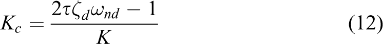
where ω_nd is the desired undamped natural frequency, and ζ_d is the desired damping coefficient, according to equation (4). As M_pd and t_sd are known, we can solve for ω_nd and ζ_d from equations (5) and (6), thus

$ζ_{d} \approx \sqrt{\frac{{(ln (M_{p d}))}^{2}}{π^{2} + {(ln (M_{p d}))}^{2}}}$
10

$ω_{n d} \approx \frac{4.6}{ζ_{d} t_{s d}}$
11

Finally, the coefficients in the denominator, the closed-loop transfer function (3), can be computed through the equivalence of the terms in the denominator of equation (9), the second-order desired transfer function. The resulting gains are now defined as

$K_{c} = \frac{2 τ ζ_{d} ω_{n d} - 1}{K}$
12

$T_{i} = \frac{K K_{c}}{τ {(ω_{n d})}^{2}}$
13

The steps of the algorithm for first-order systems without delay can be summarized as follows⁷:
Suggest M_pd and t_sd, the desired maximum overshoot and settling time.

Replace M_pd and t_sd in equations (10) and (11) to obtain ω_nd and ζ_d.

Calculate the controller gains, K_c and T_i, applying equations (12) and (13), ω_nd, ζ_d, and the system parameters K and τ.

PI controller gains for overdamped second-order processes

A representative set of industrial processes can be approximated satisfactorily by an overdamped (i.e. ζ_d > 1) second-order transfer function

$G_{2} (s) = \frac{K}{(τ_{1} s + 1) (τ_{2} s + 1)}$
14

which in turn can be seen as a combination of two first-order transfer functions in serial order.

Assuming that the PI controller defined in equation (2) is used to control a process represented by equation (14), the following closed-loop (negative feedback) transfer function results in

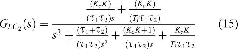
$G_{L C_{2}} (s) = \frac{\frac{(K_{c} K)}{(τ_{1} τ_{2}) s} + \frac{(K_{c} K)}{(T_{i} τ_{1} τ_{2})}}{s^{3} + \frac{(τ_{1} + τ_{2})}{(τ_{1} τ_{2}) s^{2}} + \frac{(K_{c} K + 1)}{(τ_{1} τ_{2}) s} + \frac{K_{c} K}{T_{i} τ_{1} τ_{2}}}$
15

The pole placement method is used to choose the gains K_c and T_i ¹ in the controller, described by equation (2). The denominator in equation (15), containing the gains and the parameters that describe the system, is manipulated through changing the geometrical position of the poles in the root locus. Controller gains should be chosen keeping in mind a desired pole placement; therefore proposing a closed-loop polynomial denominator.

A third pole must be added to the polynomial proposed, as the denominator in equation (15) is of third order

$D (s) = (s + p_{1}) (s^{2} + 2 ζ_{d} ω_{n d} s + ω_{n d}^{2})$
16

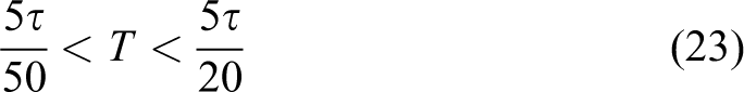
The second-order component in equation (16) can be proposed by choosing the maximum overshoot M_pd and settling time t_sd, as described before for first-order processes, meaning that it is overdamped. Certain restrictions need to be considered to propose the location of the third pole.

When it is constructing the second-order polynomial of equation (16), it is important to note that an arbitrary choice of parameters M_pd and t_sd could cause a configuration of pole locations that may turn the system unstable. There are necessary and sufficient conditions to avoid incurring in this situation, therefore that the system is stable.²⁹ These include proposing the desired settling time as

$t_{s d} > \frac{9.2 (τ_{1} τ_{2})}{τ_{1} + τ_{2}}$
17

Following the same procedure and design to calculate the gains K_c and T_i, when the process has been modeled as a second-order transfer function, mentioned previously, the terms of the denominator in equation (15) and the expanded polynomial in equation (16) are related

$K_{c} = \frac{ω_{n d}^{2} τ_{1} τ_{2} + 2 p_{1} ζ_{d} ω_{n d} τ_{1} τ_{2} - 1}{K}$
18

$T_{i} = \frac{K_{c} K}{τ_{1} τ_{2} ω_{n d}^{2} p_{1}}$
19

The algorithm for the computation of the design of a second-order system, when ζ > 1, is summarized as follows⁷:
Approximate, where it is possible, the process control structure to the form in equation (14).

Propose the maximum overshoot such that 0 < M_p < 1.

Propose t_sd according to equation (17).

Use equations (10) and (11) to calculate ζ_d and ω_nd with M_pd and t_sd previously defined.

Calculate K_c from equation (18) and T_i from equation (19).

Adaptive architecture

A PI controller that incorporates an STR explicit design structure⁵ to compute its gains was proposed by Paz Ramos et al.⁷ This STR contains an estimator of the dynamic model of the system. The controller gains are calculated by incorporating the estimated system’s parameters, during the same iteration.

The model selected for the estimation of parameters is an approximation of the structure of a continuous-time auto-regressive moving average (CARMA) controller of the form

$A Y (z) = B z^{- 1} U (z) + C ξ (z)$
20

where Y is the system’s output, U is the system’s input, and ξ is a disturbance modeled as a random sequence of uncorrelated zero mean. The coefficients A, B, and C are defined as

$\begin{array}{l} A = 1 + a_{1} z^{- 1} + a_{2} z^{- 2} + \dots + a_{n} z^{- n} \\ B = b_{0} + b_{1} z^{- 1} + b_{2} z^{- 2} + \dots + b_{n} z^{- n} \\ C = c_{0} \end{array}$
21

The parameters A, B, and C are estimated in each iteration. It is also assumed that $\hat{A} \to A, \hat{B} \to B, and \hat{C} \to C$ , that is, the estimated parameters converge to the real ones over time. Figure 1 shows the architecture of the controller.⁷

Figure 1.
Architecture of the PI controller with STR structure. PI: proportional–integral; STR: self-tuning regulator.

The recursive least squares (RLS) algorithm with exponential forgetting factor is used for the estimation, due to its extensive presence in literature and well-known advantages and disadvantages.⁷ The computation of the estimated parameters is described through the equations

$\begin{array}{l} K_{a} (k) = P (k - 1) φ (k) (λ I + φ^{T} (k) P (k - 1) φ (k {))}^{- 1} \\ \hat{θ} (k) = \hat{θ} (k - 1) + K_{a} (k) (y (k) - φ^{T} (k) \hat{θ} (k - 1)) \\ P (k) = (I - K_{a} (k) φ^{T} (k)) P (k - 1) / λ \end{array}$
22

where K_a is the adaptation gain, P is the covariance matrix, I is the identity matrix, $\hat{θ}$ is the vector estimation, φ is the regressor, λ is the exponential forgetting factor, and k is the sample in discrete time.

In order to carry out parametric estimation processes, different methods can be used; still, the use of an RLS can offer a theoretical backup from linear algebra, which allows for a supervision of the estimation process, through its covariance matrix and its inverse.^6,30

Computation of the control gains

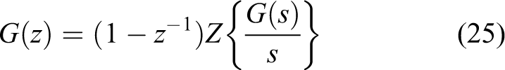
As it was previously observed in “PI controllers” section, the PI gains can be calculated using the parameters that belong to the models and the design specifications in continuous time. Nevertheless, the implementation of the adaptive version has carried out in discrete time. As part of the transformation from continuous to discrete time, the correct choice of the sampling period is very important. In this article, we used the design methodology for emulation from the study by Franklin et al.³¹ The following relation is suggested for choosing the sampling period T, when the process has been modeled with the structure presented in equation (1)

$\frac{5 τ}{50} < T < \frac{5 τ}{20}$
23

If a second-order internal model in the form of equation (14) is available, a suitable recommendation is

$T = \frac{τ_{1} + τ_{2}}{10}$
24

The controller gains can be computed from the RLS estimated parameters in a direct manner, by means of the following analysis based on the method presented in “PI controllers” section. The discrete time equivalent of a first-order transfer function obtained through a zero-order hold (ZOH) is

$G (z) = (1 - z^{- 1}) Z {\frac{G (s)}{s}}$
25

and expanding produces

$G (z) = \frac{b_{0}}{z + a_{1}}$
26

where b₀ and a₁ can be estimated by the RLS method. Applying a ZOH to equation (1), to establish a direct relation between the coefficients in equation (1) (continuous time) and the coefficients in equation (26) (discrete time), produces

$G (z) = \frac{K (1 - e^{- T / τ})}{z - e^{- T / τ}}$
27

from which it follows that

$b_{0} = K (1 - e^{- T / τ})$
28

and

$a_{1} = - e^{- T / τ}$
29

Equations (28) and (29) are solved for the time constant τ and the open-loop gain K

$τ = \frac{T}{ln (- a_{1})}$
30

$K = \frac{b_{0}}{1 - e^{- T / τ}}$
31

K and τ can be calculated directly from ${\hat{b}}_{0} and {\hat{a}}_{1}$ , in equation (21), assuming that ${\hat{b}}_{0} \to b_{0} and {\hat{a}}_{1} \to a_{1}$ .

In the case of second-order systems, it is valid to assume that the discrete ZOH computed equivalent is

$G (z) = \frac{b_{0} z + b_{1}}{z^{2} + a_{1} z + a_{2}}$
32

Applying a ZOH into the overdamped second-order system represented in equation (14), and following the same, the coefficients of the discrete form described in equation (32) can be expressed as

$b_{0} = \frac{K}{τ_{2} - τ_{1}} (τ_{2} - τ_{1} + τ_{1} e^{- T / τ_{2}} - τ_{2} e^{- T / τ_{1}})$
33

$b_{1} = \frac{K}{τ_{2} - τ_{1}} (\begin{array}{l} τ_{1} e^{- T / τ_{2}} - τ_{2} e^{- T / τ_{1}} - \\ τ_{1} e^{- T / τ_{2}} e^{- T / τ_{1}} + τ_{2} e^{- T / τ_{2}} e^{- T / τ_{1}} \end{array})$
34

$a_{1} = - e^{- T / τ_{1}} - e^{- T / τ_{2}}$
35

$a_{2} = e^{- T / τ_{1}} e^{- T / τ_{2}}$
36

In a complementary manner, the computations for the parameters in the continuous overdamped second-order system are expressed by

$τ_{2} = \frac{T}{In (- \sqrt{\frac{a_{1}^{2}}{4 a_{2}^{2}} - \frac{1}{a_{2}} - \frac{a_{1}}{2 a_{2}}})}$
37

$τ_{1} = \frac{T τ_{2}}{τ_{2} In (a_{2}) + T}$
38

$K = \frac{b_{0} (τ_{2} - τ_{1})}{τ_{2} (1 - e^{- T / τ_{2}}) - τ_{1} (1 - e^{- T / τ_{1}})}$
39

K, τ₁, and τ₂ can be computed directly from ${\hat{b}}_{0}, {\hat{b}}_{1}, {\hat{a}}_{1}, and {\hat{a}}_{2}$ from equation (21), assuming that ${\hat{b}}_{0} \to b_{0}, {\hat{b}}_{1} \to b_{1}, {\hat{a}}_{1} \to a_{1}, and {\hat{a}}_{2} \to a_{2}$ . T is a defined constant in all cases.

Finally, the algorithm for the PI controller with STR structure can be summarized as
Select the order of the internal model.

Choose the sampling period T.

Propose initial parameters.

Apply a finite duration step, in order to assist the convergence of the estimation process.

Estimate $\hat{A}, \hat{B}, and \hat{C}$ .

From $\hat{A}, \hat{B}, and \hat{C}$ , obtain K and τ if n_A = 1 or K, τ₁, and τ₂ if n_A = 2. Where n_A is the order of the polynomial.

Compute K_c and T_i.

Generate the control signal u(kT).

Implementation

As it was discussed in the first section, PID control has a preponderant presence in industrial process control. One of the main reasons for this is the fact that other control techniques require a lot more knowledge and analysis ability of the system that is being put in operation.

In order to close this gap and come up with a better-performing and more adaptive strategy, the system here proposed goes more for an automation in the design of the controller that won’t depend in its accuracy on the ability of the operator.

Implementation of this structure was thought in such a way that it could be useful in an industrial setting, since no additions of hardware have to be made to the PLC-based control loops. The controlling software just needs to be installed in the logical programmable control server, and linked to these, through the OPC communication protocol.

In order to test the performance of the controller, a testing protocol was designed, that was based on an automatized implementation of HIL, which allows the availability of information from a real plant, to perform an evaluation and an analysis of the functionality of the system working in closed loop, in the presence of induced parametric disturbances.

The methodology to compute adaptive PI controllers,⁷ explained in “Adaptive architecture” section, was tested with systems that could be satisfactorily approximated to linear first- and second-order system models. These systems were emulated with HIL. Figure 2 shows the experimental implementation for the STR and PLC, PI controller implemented using HIL, and the OPC communication scheme.

Figure 2.
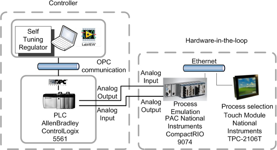
Implementation of the STR in a PLC using HIL and OPC-based communication. STR: self-tuning regulator; PLC: programmable logic controller; HIL: hardware-in-the-loop; OPC: OLE for process control.

A PLC from Allen-Bradley (Rockwell Automation), ControlLogix 5561 model, was used for PI controllers implementation. The estimation process and gain computation were implemented as MATLAB scripts within LabVIEW virtual instrumentation platform, communicating with the PLC to control the (emulated) systems. LabVIEW handles the process of signal acquisition and the industrial communication (based on the OPC standard) the NI OPC Servers tool.^22,23 The HIL emulation was performed by a real-time hardware platform, the National Instruments CompactRIO 9074 with analog modules.

The objective of a test protocol is that of offering ideal test conditions to evaluate the performance of the adaptive PI and its fixed gains.

A set point was established in the test protocol as a square signal, with a variable amplitude, which period is longer than twice the settling time in an open loop.

The following step is to perform a connection between industrial platforms. The first connection is to be performed between the PLC and the Personal Computer (PC) through an OPC, with its ethernet communication port. The second connection goes between the PLC and the PAC, through an analog output and analog input.

Once all devices have been connected, the PI adaptive program of the fixed PI gains is carried out; after three complete cycles, the parametric disturbance can be performed.

The OPC standard was developed by industrial manufacturers in order to have interoperability between different automation vendors. The main objective of OPC-based communication is the real-time interaction between different devices.³² The procedure to get connectivity between the control algorithm platform and the PLC, using the OPC standard, can be summarized in two steps: handling inputs/outputs and the manipulation of variables. To carry out the implementation of the control system described on an industrial platform with the OPC communication standard, the following algorithms must be used.
Operation of the inputs and outputs of the PLC:

Set up the protocol of communication in the PC to the PLC with RSLinx.

Register the racks of the PLC with RSLogix 5000.

Release the ladder to the PLC with RSLogix.

Shut down RSLinx.

Handling variables in LabVIEW via the OPC communication standard³³:

Establish the communication port between the device and the PC in the OPC server in NI OPC (developed by National Instruments) Servers software.

Include in NI OPC Servers the PLC tags.

Make the project in LabVIEW.

Select the OPC client in LabVIEW in the new server Input/Output (I/O).

Configure the OPC client by selecting NI OPC Servers in the LabVIEW project.

Create the bound variables.

Incorporate the variables of the OPC Server.

Allow the reading and writing for the bound variables.

Aggregate a VI file.

Program the VI in the block diagram handling the variables.

Put the PLC in run mode.

Execute the VI file.

The performance of both adaptive and conventional PI controllers was measured through the IAE, defined as

$IAE = \sum_{k = 0}^{n} | {SP}_{k} - {PV}_{k} |$
40

where SP is the set point and PV is the process variable.

Eighteen systems were tested in total, half first-order and half second-order systems, which all of them emulated by HIL. The systems were programmed as difference equations resulting from a ZOH discretization process over their transfer functions.

First-order systems were formulated differently from equation (1) as

$G_{1 α} (s) = \frac{K}{(τ + α) s + 1}$
41

using the following values: K = {0.1, 0.5, 0.8}, τ = {2, 10, 20}, and the disturbance α = {4, 10, 15}. The combination of the three different values of K and τ + α forms the first nine systems for the experiments.

Second-order systems were formulated as

$G_{2 α} (s) = \frac{K}{[(τ_{1} + α_{1}) s + 1] [(τ_{2} + α_{2}) s + 1]}$
42

with values K = {0.1, 0.5, 0.8}, τ₁ = {4, 10, 20}, τ₂ = {10, 20, 30}, and the disturbances α₁ = {3, 5, 0} and α₂ = {0, 0, 10}. The combination of the three different values of K, $τ_{1} + α_{1}, and τ_{2} + α_{2}$ forms the remaining systems for the experiments.

An advantage in the use of HIL is the repeatability of tests and the ability of testing the controller in similar conditions to those that can be found an industrial setting.

HIL allows the possibility of dynamics that go beyond simple computational simulations, since the information that is shared between the controller and the plant is not simply transferred from one register to another in a given iteration; it is rather transmitted as analogical information between the analog–digital converter of the PLC and the analog–digital port of the PAC.

It is also important to mention that the sampling periods of the different stages are not equivalent, not even in the analogical input module (1769-IF4 de Allen-Bradley) of the PLC which has a band-pass filter with the following frequencies: 50 Hz, 60 Hz, 250 Hz y 500 Hz, with a magnitude fall of −3 dB, which can be interpreted as an addition of colored noise to the closed loop.

This way, the implementation here proposed is more efficient in several aspects to computational simulation, and in itself is a test structure that can be utilized with other control strategies.

Experimental results

The implemented performance evaluation of PI controllers with an STR structure consisted of comparing their dynamic parameters (overshoot and settling time) chosen at design (“desired” dynamic behavior by specifying M_pd and t_sd), against the ones of conventional PI controllers, when following a reference signal. A disturbance is introduced in one of their parameters, at a specific time. Conventional PI controllers follow the design presented in “PI controllers” section. PI controller with an STR structure was implemented as explained in “Adaptive architecture” section.

The expected consequence of the disturbance in the systems controlled by a conventional PI is an increment in the IAE and a change in the response time. In the case of the PI with STR architecture controllers, the IAE is also expected to increase but in smaller magnitudes than in the conventional controllers. The IAE was computed in three settings: before the disturbance (at the time interval (0, d−1)), after the disturbance (at the time interval (d, n)), and throughout the experiment (time (0, n)). Tables 1 and 2 show the IAE at the intervals of time before and after the disturbance, for the first- and second-order systems, respectively. Tables 3 and 4 show the IAE throughout the experiment, for the first- and second-order systems, respectively. The results show that the magnitude of the IAE is smaller for the adaptive controller, compared to the conventional one, in most cases.

Table 1.
Integral absolute error evaluation before and after the disturbance for closed-loop first-order systems.

$\sum_{k = 0}^{d - 1} | e_{k} |$ $\sum_{k = d}^{n} | e_{k} |$

Parameters

K, τ, α PI PI PI PI

STR STR

0.1, 2, 4 19.37 18.85 51.23 25.52

0.5, 2, 4 20.98 19.67 46.61 21.25

0.8, 2, 4 22.88 20.62 52.77 21.75

0.1, 10, 10 28.41 28.32 55.18 33.27

0.5, 10, 10 28.92 28.34 52.97 33.07

0.8, 10, 10 29.42 28.59 55.65 33.41

0.1, 20, 15 10.45 11.43 15.29 12.37

0.5, 20, 15 10.45 11.39 17.78 12.38

0.8, 20, 15 10.48 11.38 17.89 14.30

PI: proportional–integral; STR: self-tuning regulator.

Table 2.
Integral absolute error evaluation before and after the disturbance for closed-loop second-order systems.

$\sum_{k = 0}^{d - 1} | e_{k} |$ $\sum_{k = d}^{n} | e_{k} |$

Parameters

$K, τ_{1}, τ_{2}, α_{1}, α_{2}$ PI PI PI PI

STR STR

0.1, 4, 10, 3, 0 6.41 8.18 9.43 7.51

0.5, 4, 10, 3, 0 6.44 8.02 9.41 7.56

0.8, 4, 10, 3,0 6.43 7.91 9.50 7.97

0.1, 10, 20, 5, 0 23.27 11.23 13.47 11.72

0.5, 10, 20, 5, 0 23.29 11.03 13.55 11.43

0.8, 10, 20, 5, 0 23.04 11.30 13.49 11.69

0.1, 20, 30, 0, 10 10.90 10.64 12.06 10.47

0.5, 20, 30, 0, 10 10.89 10.47 12.04 10.44

0.8, 20, 30, 0, 10 10.89 10.41 12.08 10.68

PI: proportional–integral; STR: self-tuning regulator.

Table 3.
Integral absolute error evaluation for closed-loop first order systems.

$\sum_{k = 0}^{n} | e_{k} |$

Parameters

K, τ, α PI PI

STR

0.1, 2, 4 70.61 44.38

0.5, 2, 4 67.59 40.94

0.8, 2, 4 75.66 42.38

0.1, 10, 10 83.59 61.60

0.5, 10, 10 81.89 61.42

0.8, 10, 10 85.08 62.01

0.1, 20, 15 25.69 23.80

0.5, 20, 15 28.24 23.78

0.8, 20, 15 28.38 25.69

PI: proportional–integral; STR: self-tuning regulator.

Table 4.
Integral absolute error evaluation for closed-loop second-order systems.

$\sum_{k = 0}^{n} | e_{k} |$

Parameters

$K, τ_{1}, τ_{2}, α_{1}, α_{2}$ PI PI

STR

0.1, 4, 10, 3, 0 15.85 15.70

0.5, 4, 10, 3, 0 15.86 15.59

0.8, 4, 10, 3, 0 15.93 15.88

0.1, 10, 20, 5, 0 36.74 22.95

0.5, 10, 20, 5, 0 36.84 22.47

0.8, 10, 20, 5, 0 36.54 22.99

0.1, 20, 30, 0, 10 22.96 21.12

0.5, 20, 30, 0, 10 22.93 20.92

0.8, 20, 30, 0, 10 22.98 21.09

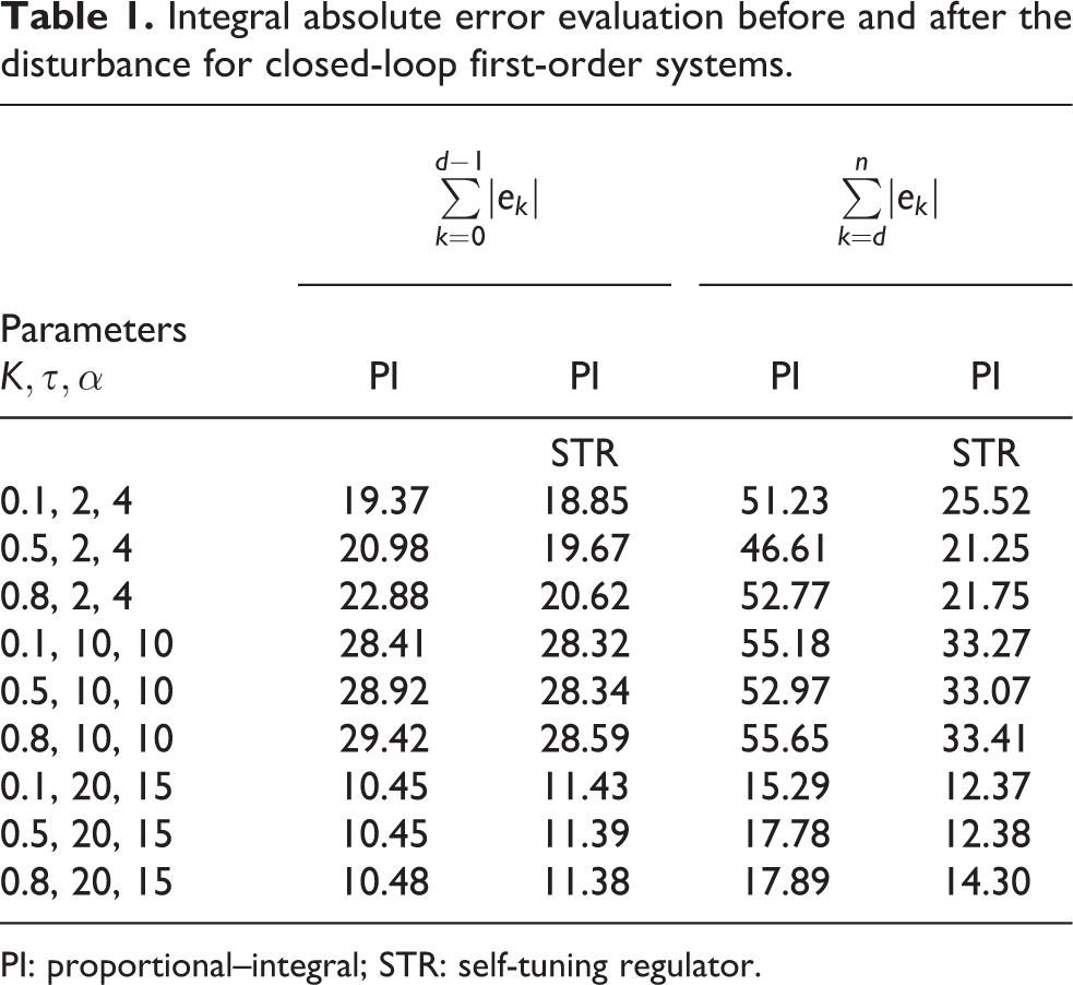
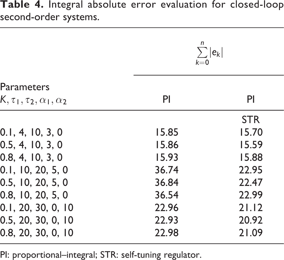
PI: proportional–integral; STR: self-tuning regulator.

The rest of this section shows an illustrative example using one of the second-order systems with parameters of $τ_{1} = 4, τ_{2} = 10, α_{1} = 3, α_{2} = 0$ , and K = 0.8 based on equation (42). The desired values for the response were of $M_{p d} = 10 % and t_{s d} = 45$ s. The selected sampling period for the discretization was 2 s. For the estimation, the initialization values were $P_{0} = 5000 I, θ_{0} = [0, 0, 0, 0]$ , and λ = 0.985. For the conventional PI controller, with K = 0.8, the values of the controller gains were K_c = 1.7330 and T_i = 7.9635. The disturbance appeared at 960 s.

Figures 3 and 4 show the behavior of the estimations over time. A small estimation error is observed. When the disturbance is triggered, the gains in the controller are also modified. This allows for a better approximation to the reference signal, in closed loop, by modifying the control signal.

Figure 3.
Estimation of parameters a₁ and a₂ for a second-order system.

Figure 4.
Estimation of parameters b₀ and b₁ for a second-order system.

The performance of a PI controller with an STR structure is shown in Figure 5(a). The internal structure of the estimator computes a second-order CARMA difference equation. The output signal PI-STR is close to one chosen in design (desired response), according to the settling time.

Figure 5.
(a) Performance of PI controller with an STR structure and (b) performance of PI controller. PI: proportional–integral; STR: self-tuning regulator.

Figure 5(b) shows the performance of a conventional PI controller in closed loop, which conforms to the parameters specified in the design stage (desired behavior) before the disturbance occurs. The disturbance causes deterioration in the output PI when tracking the reference. The observed change in the systems response when the disturbance appears is due to a migration of the poles of the closed-loop system (i.e. the systems parameters have changed), while the gains of the controller remained constant. After the disturbance, the controller generates a signal with more overshoot and even more settling time (longer time than desired), thus the desired performance criteria is not reached anymore.

Conclusion

In this article, an implementation of an adaptive (STR) PI controller architecture was presented and evaluated. The STR structure allows to adapt the controller parameters to accomplish a good performance according to the settling time desired and adjust in order to face changes in system parameters. The implementation involves the use of available hardware platforms (PLCs), connected to a PC to perform the adaptive computations, and communicating through the OPC standard. This allows a more feasible implementation of modern control techniques in different applications in process control, manufacturing, and robotics, employing general use hardware platforms instead of application-dependent equipment.

The performance of the implemented adaptive PI controller architecture was compared against conventional PI controllers, also implemented in the same hardware. The gains of the conventional PI controllers were tuned by pole assignment, from a proposed desired dynamic response. The adaptive PI controllers employ estimation of system’s parameters to compute the gains. This experimental setup served two main purposes: demonstrating the feasibility of controlling systems in OPC-based architectures, teamed with industrial hardware platforms (e.g. PLCs); and demonstrating the performance of adaptive PI controllers against conventional PI ones, in the presence of disturbances. Nineteen controllers were designed and implemented, for the first- and second-order systems emulated by HIL. Their dynamic performance was evaluated, by measuring the IAE with respect to the desired behavior from design, in the presence of a disturbance. Adaptive PI controllers performed better than the conventional ones.

	$\sum_{k = 0}^{d - 1} \| e_{k} \|$	$\sum_{k = d}^{n} \| e_{k} \|$
		STR		STR
0.1, 2, 4	19.37	18.85	51.23	25.52
0.5, 2, 4	20.98	19.67	46.61	21.25
0.8, 2, 4	22.88	20.62	52.77	21.75
0.1, 10, 10	28.41	28.32	55.18	33.27
0.5, 10, 10	28.92	28.34	52.97	33.07
0.8, 10, 10	29.42	28.59	55.65	33.41
0.1, 20, 15	10.45	11.43	15.29	12.37
0.5, 20, 15	10.45	11.39	17.78	12.38
0.8, 20, 15	10.48	11.38	17.89	14.30

	$\sum_{k = 0}^{d - 1} \| e_{k} \|$	$\sum_{k = d}^{n} \| e_{k} \|$
		STR		STR
0.1, 4, 10, 3, 0	6.41	8.18	9.43	7.51
0.5, 4, 10, 3, 0	6.44	8.02	9.41	7.56
0.8, 4, 10, 3,0	6.43	7.91	9.50	7.97
0.1, 10, 20, 5, 0	23.27	11.23	13.47	11.72
0.5, 10, 20, 5, 0	23.29	11.03	13.55	11.43
0.8, 10, 20, 5, 0	23.04	11.30	13.49	11.69
0.1, 20, 30, 0, 10	10.90	10.64	12.06	10.47
0.5, 20, 30, 0, 10	10.89	10.47	12.04	10.44
0.8, 20, 30, 0, 10	10.89	10.41	12.08	10.68

	$\sum_{k = 0}^{n} \| e_{k} \|$
		STR
0.1, 2, 4	70.61	44.38
0.5, 2, 4	67.59	40.94
0.8, 2, 4	75.66	42.38
0.1, 10, 10	83.59	61.60
0.5, 10, 10	81.89	61.42
0.8, 10, 10	85.08	62.01
0.1, 20, 15	25.69	23.80
0.5, 20, 15	28.24	23.78
0.8, 20, 15	28.38	25.69

	$\sum_{k = 0}^{n} \| e_{k} \|$
		STR
0.1, 4, 10, 3, 0	15.85	15.70
0.5, 4, 10, 3, 0	15.86	15.59
0.8, 4, 10, 3, 0	15.93	15.88
0.1, 10, 20, 5, 0	36.74	22.95
0.5, 10, 20, 5, 0	36.84	22.47
0.8, 10, 20, 5, 0	36.54	22.99
0.1, 20, 30, 0, 10	22.96	21.12
0.5, 20, 30, 0, 10	22.93	20.92
0.8, 20, 30, 0, 10	22.98	21.09

Footnotes

Declaration of conflicting interests

The author(s) declared no potential conflicts of interest with respect to the research, authorship, and/or publication of this article.

Funding

The author(s) disclosed receipt of the following financial support for the research, authorship and/or publication of this article: The author(s) received financial support of Polytechnic University of Aguascalientes for the publication of this article.

References

Astrom

Hagglund

. PID controllers: Theory, design and tuning. United States of America: ISA, 1995.

Bennet

. Development of the PID controller. IEEE Control Syst Magaz 1993; 13(6): 58–65.

O’Dwyer

. PI and PID controller tuning rules: an overview and personal perspective. In: Proceedings of the IET Irish Signals and Systems Conference, Dublin Institute of Technology, Dublin, Ireland, June 2006, pp. 161–166. The Institution of Engineering and Technology. http://www.theiet.org/

Astrom

. Adaptive control around 1960. IEEE Control Syst 1996; 16(3): 44–49.

Astrom

Wittermark

. Adaptive control. Boston: Addison-Wesley, 1995.

Wellstead

Zarrop

. Self-tuning systems: Control and signal processing. England: Wiley, 1991.

Paz Ramos

Garibo Esquivel

DeLuna-Ortega

. PI controller with dynamic gains calculation to comply time specs in presence of parametric disturbance. In: 8th International conference on electrical engineering computing science and automatic control, Toluca, México, 10–13 November 2009, pp. 322–327. IEEE. https://www.ieee.org/

Ponce Cruz

Paz Ramos

Fernández del Busto

. DTC scheme for an induction motor using generalized minimum variance controller with dynamic pole assignment. In: Proceedings of the IEEE international symposium on industrial electronics, Dubrovnik, Croatia, 20–23 June 2005, pp. 957–962. IEEE. https://www.ieee.org/.

Sharifi

Behzadipour

Vossoughi

. Model reference adaptive impedance control in Cartesian coordinates for physical human robot interaction. Adv Robot 2014; 28(19): 1277–1290.

10.

Zhang

Wei

. Design, analysis and modelling of a hybrid controller for serial robotic manipulators. Robotica 2017; 35(1): 1888–1905.

11.

Tran

Hei

. Adaptive control for an uncertain robotic manipulator with input saturations. Control Theory Technol 2016; 14(2): 113–121.

12.

Takatsy

Itoh

. Future needs for control theory in industry report of the control technology survey in Japanese industry. IEEE Trans Control Sys Technol 1999; 7(3): 298–305.

13.

Rhinehart

. The century’s greatest contributions to control practice. ISA Trans 2000; 39(1): 3–13.

14.

Desborough

Nordh

Miller

. Control system reliability: process out of control. In: InTech, 2001, pp. 52–55. https://ww2.isa.org/intech/; http://www.loopscout.com/Info/Intech.pdf

15.

Anbarasi

Muralidharan

. Enhancing the transient performances and stability of AVR system with BFOA tuned PID controller. J Control Eng Appl Inform 2016; 18(1): 20–29.

16.

Creus

. Instrumentacin industrial. Instrumentacion, Spain: Marcombo, 2005.

17.

Kocian

Koziorek

. An outline of advanced process control and self-tuning techniques on PLC background. In: Conference on emerging technologies and factory automation (ETFA), Toulouse, France, 5–9 September 2011, pp. 1–8. IEEE. https://www.ieee.org/

18.

Vijayalakshmi

Manamalli

PalaniKumar

. Closed loop experimental validation of linear parameter varying model with adaptive PI controller for conical tank system. J Control Eng Appl Inform 2014; 16(4): 12–19.

19.

Mendes

Araujo

Sousa

. An architecture for adaptive fuzzy control in industrial environments. Comput Indus 2011; 62(3): 364–373.

20.

Mahnke

Leitner

. OPC unified architecture. Springer, 2009.

21.

Pendli

Gorbatchev

Schwarz

. OPC and its strategies for redundancy. In: Proceeding of the 10th WSEAS international conference on communications, Athens, Greece, 13–15 July 2006, pp. 163–168. World Scientific and Engineering Academy and Society. www.wseas.org/

22.

Paz Ramos

Avila Alonso

García Barberi

. Sintonización de controladores PID vía OPC. In: 6to Congreso Internacional sobre Innovación y Desarrollo Tecnológico CIINDET 2008, Cuernavaca, México, 8–10 October 2008. IEEE Morelos. http://ieeemorelos.org/index.html/

23.

Paz Ramos

Velázquez Alvarez

Valencia Maza

. Detector de algoritmos de control PID vía OPC. In: 6to Congreso Internacional sobre Innovación y Desarrollo Tecnológico CIINDET 2008, Cuernavaca, México, 8–10 October 2008. IEEE Morelos. http://ieeemorelos.org/index.html

24.

MacNeal

Belkhayat

. Standard tools for hardware-in-the-loop (HIL) modeling and simulation. In: Electric ship technologies symposium, Arlington, VA, USA, 21–23 May 2007, pp. 130–137. IEEE. https://www.ieee.org/

25.

Munteanu

Bratcu

Bacha

. Hardware-in-the-loop-based simulator for a class of variable-speed wind energy conversion system: design and performance assessments. IEEE Trans Energy Convers 2010; 25(2): 564–576.

26.

Martin

Emami

. Dynamic load emulation in hardware-in-the-loop simulation of robot manipulators. IEEE Trans Indus Elect 2011; 58(7): 2980–2987.

27.

Shinsky

. Process control systems application, design, and tuning. United States of America: McGraw-Hill, 1998.

28.

Bissel

. Control engineering. England: Chapman and Hall, 1994.

29.

Paz

Ramirez-delreal

Garibo

. Algoritmo didáctico para la asignación implícita de polos mediante la especificación de características temporales deseadas usando controladores PI industriales. Formación Universitaria 2013; 6(6): 23–40.

30.

Isermann

Lachmann

. Parameter-adaptive control with configuration aids and supervision functions. Automatica 1995; 21(6): 625–638.

31.

Franklin

Poweill

Workman

. Digital control of dynamic systems. Addison-Wesley, 1998.

32.

Santori

M. OPC

: OLE for process control. Real-Time Magaz 1997; 97(4): 78–81.

33.

United States of America, National-Instruments. Help contents de NI OPC servers, 2009. http://www.ni.com/tutorial/4626/en/

	$\sum_{k = 0}^{d - 1} \| e_{k} \|$		$\sum_{k = d}^{n} \| e_{k} \|$
Parameters
K, τ, α	PI	PI	PI	PI
		STR		STR
0.1, 2, 4	19.37	18.85	51.23	25.52
0.5, 2, 4	20.98	19.67	46.61	21.25
0.8, 2, 4	22.88	20.62	52.77	21.75
0.1, 10, 10	28.41	28.32	55.18	33.27
0.5, 10, 10	28.92	28.34	52.97	33.07
0.8, 10, 10	29.42	28.59	55.65	33.41
0.1, 20, 15	10.45	11.43	15.29	12.37
0.5, 20, 15	10.45	11.39	17.78	12.38
0.8, 20, 15	10.48	11.38	17.89	14.30

	$\sum_{k = 0}^{d - 1} \| e_{k} \|$		$\sum_{k = d}^{n} \| e_{k} \|$
Parameters
$K, τ_{1}, τ_{2}, α_{1}, α_{2}$	PI	PI	PI	PI
		STR		STR
0.1, 4, 10, 3, 0	6.41	8.18	9.43	7.51
0.5, 4, 10, 3, 0	6.44	8.02	9.41	7.56
0.8, 4, 10, 3,0	6.43	7.91	9.50	7.97
0.1, 10, 20, 5, 0	23.27	11.23	13.47	11.72
0.5, 10, 20, 5, 0	23.29	11.03	13.55	11.43
0.8, 10, 20, 5, 0	23.04	11.30	13.49	11.69
0.1, 20, 30, 0, 10	10.90	10.64	12.06	10.47
0.5, 20, 30, 0, 10	10.89	10.47	12.04	10.44
0.8, 20, 30, 0, 10	10.89	10.41	12.08	10.68

Adaptive proportional–integral controller using OLE for process control for industrial applications

Abstract

Keywords

Introduction

PI controllers

PI controller gains for first-order processes

PI controller gains for overdamped second-order processes

Adaptive architecture

Computation of the control gains

Implementation

Experimental results

Conclusion

Footnotes

Declaration of conflicting interests

Funding

References