Sage Journals: Discover world-class research

Abstract

This article presents a new approach for planning collision-free trajectories of two robots working in a shared workspace. Based on the B-spline knot refinement and the local modification scheme, the approach only changes the local trajectory around the collision area without changing the shape in the global way. The geometric model of dual-robot is employed by two kinds of geometric elements (sphere and capsule). A collision check method calculates the distance between two robots to determine whether the collisions exist. The collision check is converted to calculate the distance between every two elements. The proposed method has been implemented on a dual-robot system composed of two KUKA manipulators. The numerical and simulation results presented in the article illustrate the efficiency of the proposed technique.

Keywords

Collision free dual robot collision checking trajectory planning B-spline

Introduction

Dual or multiple robots are employed in many industrial areas from simple material handling to complex assembly. For a dual-robot or multi-robot system in a shared workspace, it is necessary to ensure the robots to move safely without collisions. Collision-free techniques tend to be based on speed adaptation, path deviation by one robot only, path deviation by two robots, or a combination of speed and path adjustments.

In the literature, many different techniques for collision-free trajectory planning of a dual-robot system have been proposed. Shin and Zheng decomposed collision-free multi-robot motion planning into two sequential steps, path planning and trajectory planning, and obtained the time optimality of dual-robot collision-free trajectory planning by delaying one of the two robots.¹ Ju et al. proposed a velocity alteration strategy to account for collision avoidance between links.² Spencer et al. presented the input velocity scaling where the path of the robot is not modified, but the motion of the robot along the desired path is slowed in order to avoid collisions.³ Each of these methods is essentially velocity schedule along a prior planned path. To generate a collision-free trajectory, the velocity of the slave robot is reduced or waiting time intervals in slave robot trajectory are inserted. However, such a method is only effective if the obstacles will move out of the path of the robot after a period of time and makes the robot less efficient.

Lee and Lee developed notions of collision map and time scheduling for realizing a collision-free motion planning.⁴ In order to avoid collisions, Chu and ElMaraghy applied heuristic rules to modify the robot path.⁵ Cai et al. developed a step-forward approach for collision avoidance in multi-robot systems.⁶ Some work on the general collision-free robot navigation problem can also be seen in the study by Hoy et al.,⁷ Cho and Cho,⁸ and Ouyang and Zhang.⁹ The robot must change its established path to avoid collisions with static obstacles. For dynamic obstacles, the lower priority robot took a “stopping” or “speed reduction” action to avoid a collision. Path deviations are adopted in these methods. The prior planned trajectories are often optimal according to some objectives. The range and the adjustment of the path deviation should be small enough to avoid collisions and to keep the trajectories as well as possible, which are not considered sufficiently in these articles.

The trajectory planning for a dual-robot system is different from that of a single robot in that each robot is a moving obstacle to the other robot. In a single robot, many trajectory planning techniques are adopted. Parametric curves build the trajectory due to their useful properties. The most commonly used curves are multi-order spline,^10,11 Bezier, and^12,13 B-spline.^14,15 Trajectory planning algorithms found in the literature aim at minimizing some objective function,^16
–18 which are usually execution time, actuator effort, and jerk.

B-spline techniques can realize a fast response to moving obstacles in an environment. Changing one point of the control polygon only affects the corresponding curve locally. Focusing on the performance of sudden changes in a predefined trajectory, Dyllong and Visioli investigated various spline techniques for planning and fast modifications of a trajectory of robot manipulators.¹⁹ Fast changes at a joint level can be implemented by using B-splines. Arney employed an interpolated B-spline to the waypoints, which is only altered in the local area to the obstacle.²⁰ Shukla et al. proposed a B-spline for the manipulator path which leads to effective collision avoidance.²¹ However, one or more control points are changed to modify the path. The range of the path deviation is often relatively wide.

The main contributions of this work are that,

A collision-free trajectory planning algorithm strategy for dual-robot working in a shared workspace is proposed. This strategy modifies the trajectory curve around the collision area using the B-spline knot refinement and local modification scheme.

The harmony search (HS) algorithm is used to obtain optimal trajectory planning. In order to avoid collision, the HS algorithm is applied to get the adjusting directions and values of joints.

An approach of collision checking is presented by employing the geometric models of robots.

Model building and collision checking

The dual-robot system is composed of two 6-degree of freedom (6-DOF) industrial robots, R1 and R2, working in a shared workspace. The reference frame of the dual-robot system is T ₀ and the base frames of R1 and R2 are T ₀₁ and T ₀₂, respectively. The coordinate systems of the dual-robot system are shown in Figure 1. In the reference frame T ₀, the position of points on robots R1 and R2 can be denoted as $p_{0}^{01}$ and $p_{0}^{02}$ , respectively

p_{0}^{01} = T_{0}^{01} p_{01}

p_{0}^{02} = T_{0}^{02} p_{02}

Figure 1.

The coordinate systems of a dual-robot system.

where p₀₁ is the position vectors of points on robot R1 in base frame T ₀₁; p₀₂ is the position vectors of points on robot R2 in base frame T ₀₂; $T_{0}^{01}$ is the transformation matrix of the base frame T ₀₁ with respect to reference frame T ₀; $T_{0}^{02}$ is the transformation matrix of the base frame T ₀₂ with respect to reference frame T ₀.

The two robot positions can be expressed uniformly in the reference frame T ₀ via equations (1) and (2). They can be used to calculate the distance to judge if there is collision between the two robots.

As the links and joints of a 6-DOF robot are irregular and complex, in order to calculate the distance between two robots, it is necessary to model the robot links and joints by geometric primitives. Sphere and capsule (composed of a cylinder and two hemispheres in the ends of the cylinder) are adopted as geometric primitives in this article. The wrist is modeled by the sphere S and the links are modeled by the capsules C₁, C₂, and C₃, as shown in Figure 2(a). As the former three links determine the position of the robot end-effector and the last three links only affect the orientation of the robot end-effector, it is the angular positions of first three joints that determine whether the robots collide. Hence, the 6-DOF robot can be simplified as a three-DOF robot, as shown in Figure 2(b).

Figure 2.

Geometric model of a dual-robot system.

The safety margin to avoid a collision between two robots is defined as the minimum necessary distance between two robots. Given the minimum necessary safety distance d_s (≥0), a robot trajectory must obey the following constraint

d_{s} \geq v T

where the braking time T possibly depends on the robot payload,²² the velocity v is the joint velocity.

The distance r between the robots R1 and R2 is

r = min {| e_{1, i} - e_{2, j} |, i = 1, 2, 3, 4; j = 1, 2, 3, 4}

where e_a,b denotes the bth primitive of the robot a. The condition for collision avoidance is r ≥ d_s. Fulfilling this criterion means that the robots will never meet in the same region by defining a circle with the radius d_s, which is called a non-overlapping criterion.

According to the geometric model of a robot, the distance between the two robots can be converted to distances between primitives, as shown in Figure 3. The minimum distance between a pair of objects is called the critical distance. The distance between centers or axes of the geometric primitives (spheres or capsules) is L. The radii of the primitives are r_A and r_B, respectively. If there is $| L - r_{A} - r_{B} | > d_{s}$ , the primitives do not overlap. If all the primitives of the two robots do not overlap, the two robots will not collide.

Figure 3.

Distance between two geometric elements.

Trajectory planning for robots based on B-spline curves

Assuming that the path in the Cartesian space consists of a sequence of via-points (positions and orientations of the end-effector), the robot has f joints, there are m+1 via-points for each joint, and T is the total time for traveling from the first via-point to the last one.

B-spline curves are used to formulate the jth joint trajectory, which can be expressed as

Q_{j} (u) = \sum_{i = 0}^{n} N_{i, p} (u) \cdot P_{i, j}, j = 1, 2, \dots, f

with

{\begin{matrix} N_{i, 0} (u) = {\begin{matrix} 1, if u_{i} \leq u \leq u_{i + 1} \\ 0, otherwise \end{matrix} \\ N_{i, p} (u) = \frac{u - u_{i}}{u_{i + p} - u_{i}} N_{i, p - 1} (u) + \frac{u_{i + p + 1} - u}{u_{i + p + 1} - u_{i + 1}} N_{i + 1, p - 1} (u) \end{matrix}

where P_i,j is the ith control point of the jth joint B-spline trajectory, n+1 is the number of control points, and the pth order polynomial N_i,p(u) is the B-spline basis function defined on the nonuniform knot vector $U = {u_{0}, u_{1}, \dots, u_{k}, u_{k}_{+ 1}, \dots, u_{n}_{+ p + 1}}$ .²¹

The knot vector U can be obtained by parameterizing and normalizing the interval time Δt_i, and the knot vector repetition degree in both ends is p+1

\begin{array}{l} u_{i} = u_{i - 1} + \frac{Δ t_{i - p + 1}}{T}, i = p + 1, p + 2, \dots, n \\ u_{0} = u_{1} = \dots = u_{p} = 0 \\ u_{n + 1} = u_{n + 2} = \dots = u_{n + p + 1} = 1 \end{array}

The trajectory must pass through m+1 via-points, and the corresponding B-spline curve has m segments. The expression of ith segment is described as

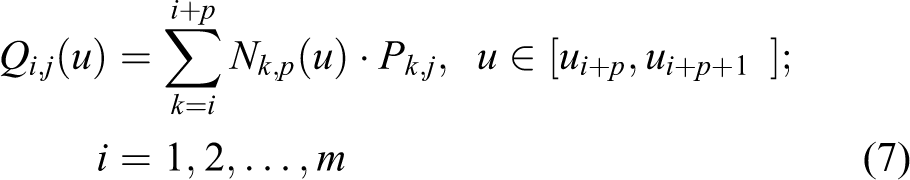
Q_{i, j} (u) = \sum_{k = i}^{i + p} N_{k, p} (u) \cdot P_{k, j}, u \in [u_{i + p}, u_{i + p + 1}]; i = 1, 2, \dots, m

The n+1 control points P_i,j can be obtained by solving n+1 equations which consist of interpolation conditions in equation (7) and boundary conditions in equation (8). The interpolation conditions contain m+1 equations

q_{i}^{j} = Q_{i, j} (u_{i + p}) = \sum_{k = i}^{i + p} N_{j, p} (u_{i + p}) \cdot P_{k, j}, i = 1, 2, \dots, m

where $q_{i}^{j}$ is the ith via-point position value of the jth joint.

Given Δt_i, the control points can be computed by solving n+1 equations consisting of equations (6) and (7), and control points of the derivative curve can be obtained by equation (8). Then, the trajectories of robot joints constructed by B-spline curves are obtained.

Collision-free trajectory planning for a dual-robot system

The B-spline trajectory of a manipulator can be obtained by applying the above proposed trajectory planning algorithm. The trajectories of robots R1 and R2 are S1 and S2, respectively. The two robots may collide when they move along the trajectories S1 and S2. In this case, the trajectories should be modified to avoid the collision. There are methods which modify the whole trajectory to avoid collisions. In this article, the trajectory is partly modified to avoid collisions by applying the local modification scheme of B-spline curves. B-spline curves have local modification scheme property: changing the position of control point P_i only affects the curve Q(u) on the interval [u_i , u_i _+p+1]. We can modify a curve locally without changing the overall shape.

Both the trajectories can be modified to avoid collisions. A trajectory which will be modified is determined according to the priority. If one robot needs higher efficiency or accuracy, its priority is higher, otherwise they are the same priority. The higher priority trajectory will not be changed such that much more important trajectories remain unchanged, while the less important one is modified. If they have the same priority, either of them can be modified.

In order to less modify the trajectory, the knot refinement of B-splines is implemented. Knot refinement or knot insertion is exactly what the name suggests: extension of a given knot vector by adding new knots.

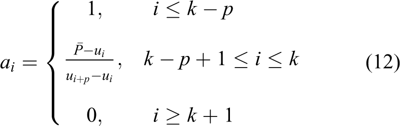
Before modifying the trajectory, we refine the trajectory around the collision area so that the affected area could be restricted to a narrow region. According to the demand, the knot refinement could be accomplished by inserting one or several knots. The method of inserting a knot is detailed as follows.

For convenience, $Q (u) = \sum_{i = 0}^{n} N_{i, p} (u) \cdot P_{i}$ is used to make a general reference to a joint trajectory. It is checked at every sample time whether there is a collision between the robots. The time t′ when a collision occurs is recorded. A new knot $\bar{u} = (t^{'} \pm λ) / T$ (t′ ± λ denotes a moment around the time t′ and λ could be given according to T) is inserted into the nonuniform knot vector U to generate a new nonuniform knot vector $\bar{U}$ via equation (4). Assuming $\bar{u} \in [u_{k}, u_{k + 1}], 0 \leq k < n + p + 1$ , the knot vector $\bar{U}$ is as follows

\bar{U} = {{\bar{u}}_{0} = u_{0}, \dots, {\bar{u}}_{k} = u_{k}, {\bar{u}}_{k + 1} = \bar{u}, {\bar{u}}_{k + 2} = u_{k + 1}, \dots, {\bar{u}}_{n + p + 2} = u_{n + p + 1}}

Q(u) could be expressed with the knot vector $\bar{U}$

Q (u) = \sum_{i = 0}^{n + 1} {\bar{N}}_{i, p} (u) {\bar{P}}_{i}

where ${\bar{N}}_{i, p}$ are the pth-order B-spline basis functions defined on the knot vector $\bar{U}$ and ${\bar{P}}_{i}$ are the new control points after inserting the new knot

{\bar{P}}_{i} = a_{i} P_{i} + (1 - a_{i}) P_{i - 1}

where

a_{i} = {\begin{matrix} 1, & i \leq k - p \\ \frac{\bar{P} - u_{i}}{u_{i + p} - u_{i}}, & k - p + 1 \leq i \leq k \\ 0, & i \geq k + 1 \end{matrix}

After refining the trajectory, the control points are adjusted to fine-turn the shape of the trajectory around the time t′, while the remaining curve segments of the trajectory stay in their original place without any change. We only need to recheck the partial modified trajectory to determine whether there is a collision. If there is no collision, the whole trajectory is collision free. If there is a collision, the control point is adjusted repeatedly till no collision occurs. Assuming that P′ is the control point that will be adjusted, ΔP is the value of the control point adjusted one time, d(P′) and d(P′ + ΔP) are the distances between two robots. The following pseudo codes describe the process of adjusting the control point. The procedure of the collision-free trajectory planning is shown in Figure 4.

if $d (P^{'} + Δ P) < d (P^{'})$ // The distance decreases when the control point P′ adds ΔP

δ = ΔP // The adjusting direction is the same with the joint moving direction

else // The distance decreases when control point P′ subtracts ΔP

δ = −ΔP // The adjusting direction is opposite to the joint moving direction

while d(P′) < d_s // Adjust the control point repeatedly till the distances are larger than d_s

P′ = P′ + δ // Adjust δ every time

Figure 4.

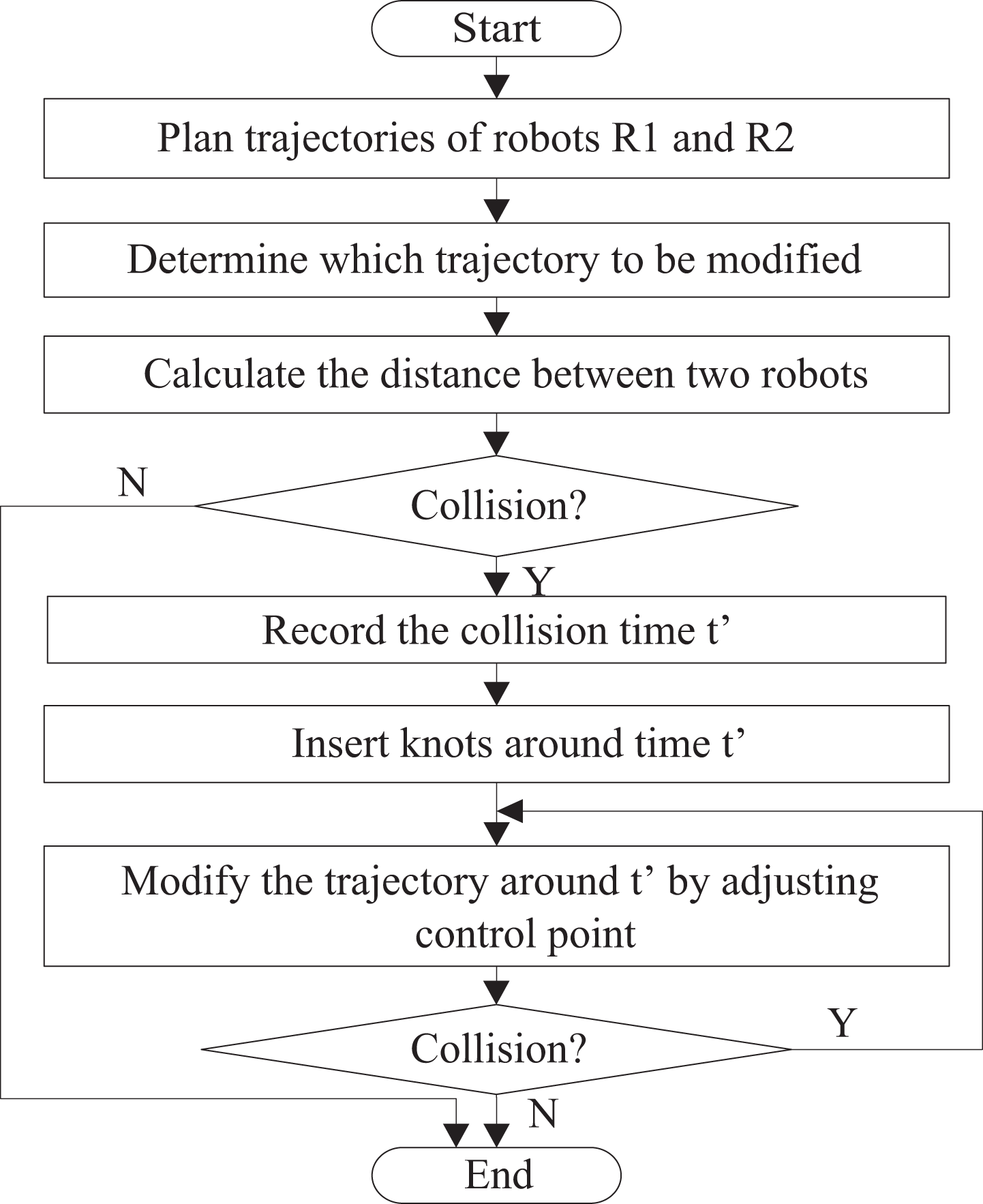
Procedure of the collision-free trajectory planning.

The adjusting directions and values of multiple joints are not straightforward to determine. Some optimization algorithms, for example, the HS algorithm, can be applied. The HS imitates the music improvisation process where music players search for a better state of harmony.²³ The HS can be used to obtain optimal trajectory planning.²⁴ The HS can determine the optimal result and is convergent. There have been improvements in order to avoid the HS falling into local minimal.²⁵ The algorithm is less of a computational load than other heuristic algorithms.²⁶ The HS is applied to obtain the adjusting values and directions.

Assuming that the robot has n joints. Without loss of generality, we assume that only one control point of each joint trajectory should be changed, and P_i is the control point that will be adjusted for the ith joint trajectory. The detailed processes are described as follows:

Step 1: Initialize the optimization problem and algorithm parameters.

The optimization problem is defined as

D = D (X) = | min (d (x_{i}, t) - d_{s} - d_{0}) |, x_{i} \in [x_{i L}, x_{i u}], i = 1, 2, \dots, n

where x_i = ΔP_i is the adjusted value of the control point of ith joint trajectory. x_iL and x_iu are the lower and upper bounds for variables which are determined by P_i, respectively. The limits of the joints d₀(> 0) are an extra term to make d(x_i,t)−d_s always positive, which will be proved later.

The HS algorithm parameters are the number of decision variables, bandwidth bw, the harmony memory size HMS, the harmony memory considering rate HMCR, the pitch adjusting rate PAR, and the stopping criterion D(X_best) < d₀.

Step 2: Initialize the harmony memory:

H M = (\begin{matrix} x_{1}^{0} & \dots & x_{n}^{0} \\ ⋮ & ⋱ & ⋮ \\ x_{1}^{H - 1} & \dots & x_{n}^{H - 1} \end{matrix})

x_{i}^{k} = max (x_{i L}) + rand () \times (min (x_{i U}) - max (x_{i L}))

where $X_{k} = (x_{1}^{k}, x_{2}^{k}, \dots, x_{n}^{k})$ is the kth solution vector.

Step 3: Execute the local search.

Find the best solution vector and the worst one

D (X_{best}) = min (D (X_{k})), D (X_{worst}) = max (D (X_{k}))

Then, execute the feasible direction method to obtain the local optimal solution vector X′, using the vector V = X_best − X_worst as the search direction. Finally, replace X_worst with X′.

Step 4: Improvise a new harmony with three different mechanisms: memory consideration, pitch adjustment, and random selection.

Step 5: Harmony memory update. If D(X_new) < D(X_worst), replace X_worst with X_new.

Step 6: Repeat steps 3–5 until the stopping criterion is satisfied.

Step 7: Find the best harmony vector X_best in the final HM as the global optimal solution vector.

Now, we prove d(X_best,t) > d_s. From the stopping criterion, D(X_best) < d₀, that is

| min_{t} (d (X_{best}, t) - d_{s} - d_{0}) | < d_{0}

d_{s} < min_{t} (d (X_{best}, t)) < d_{s} + 2 d_{0}

Obviously, $min_{t} (d (X_{best}, t)) < d (X_{best}, t)$ . So $d (X_{best}, t) > d_{s}$ .

Additionally, we can tag on velocity or jerk constraints in the stopping criterion to obtain smoother trajectories.

Simulation

To show the validity of the proposed collision-free trajectory planning approach, a case study of two KUKA KR1000_TITAN robots is carried out. The robot Denavit-Hartenberg (DH) parameters are detailed in Table 1. The transformation matrixes of the base frame T ₀₁ and T₀₂ with respect to the reference frame T ₀ are $T_{0}^{01}$ and $T_{0}^{02}$ respectively, where

Table 1.

Link parameters of KR1000_TITAN.

	d (mm)	α (°)	a (mm)	θ (°)
1	0	0	1100	θ1
2	600	−90	0	θ2
3	1400	0	0	θ3
4	65	90	1200	θ4
5	0	−90	0	θ5
6	0	90	372	θ6

T_{0}^{01} = [\begin{matrix} 1 & 0 & 0 & 0 \\ 0 & 1 & 0 & 0 \\ 0 & 0 & 1 & 1000 \\ 0 & 0 & 0 & 1 \end{matrix}], T_{0}^{02} = [\begin{matrix} 1 & 0 & 0 & 0 \\ 0 & 1 & 0 & 4200 \\ 0 & 0 & 1 & 1000 \\ 0 & 0 & 0 & 1 \end{matrix}]

Assuming that R1 and R2 have the same priority. R1 moves from the point E1(0,860,3600) to the point F1(0,3360,2150) and R2 moves from the point E2(0,3140,3600) to the point F2(0,3360,650) in the Cartesian space. As shown in Table 2, the joints’ positions of starting point and end point are obtained by inverse kinematics. Assuming that the start and end velocities are set to zero, and the total time is 3.5 s, the trajectories of R1 and R2 (in Figure 5) are built with cubic B-splines on knot vectors U ₁ = {0, 0, 0, 0,0.4,0.5, 1, 1, 1, 1} by applying the trajectory planning algorithm for a single robot.

Table 2.

The starting and end point in joint space.

Position	Robot R1			Robot R2
Position	Joint 1	Joint 2	Joint 3	Joint 1	Joint 2	Joint 3
Starting point (°)	90	15.1772	−153.6340	90	−177.0470	−3.0676
End point (°)	90	24.2294	43.9277	90	−119.2130	35.1794

Figure 5.

Position of robots R1 and R2.

The robot geometric model is built with the elements of sphere and capsule, and the element dimensions are given according to the robot physical dimension. The radii of the sphere, the hemispheres in the capsules ends, and the length of the capsules central segments are shown in Table 3. The distances between two robots (shown in Figure 6) are calculated by applying the collision checking method presented in the section “Model building and collision checking.” As Figure 6 (blue color dotted line) shows, R1 and R2 are closest at t′ = 2.38 s and the distances between 2.17 s and 2.66 s are smaller than 0 (here d_s is simplified as zero), so there are collisions in the period between 2.17 s and 2.66 s.

Table 3.

The elements’ geometric dimensions.

Geometric dimensions	Sphere	Capsule
Geometric dimensions	S	C₁	C₂	C₃
Radius (r/mm)	372	350	300	300
Central segment (l/mm)	—	830	1400	1200

Figure 6.

Distance between R1 and R2 before and after modifying trajectories with case 1.

In order to obtain collision-free trajectories, we need to modify the obtained trajectories. Assuming that robots R1 and R2 have the same priority, it is available to modify one robot trajectories or the trajectories of both R1 and R2. Two cases of adjusting trajectories are implemented and compared. We insert three knots around the collision, and the knot vectors are ${\bar{U}}_{1} = {0, 0, 0, 0, 0.4, 0.5, 0.7, 0.8, 0.9, 1, 1, 1, 1}$ . We get the new control points by employing equations (11) and (12) and obtain the modified trajectories using equation (10). The adjusting values and directions of control points for each joint are implemented by the HS algorithm. In the first case, the local modification of B-splines with knot refinement is compared with that without knot refinement.

Case 1: Only modify the trajectories of R2, the trajectories of Robot R1 stay in the original shape. Apply the collision-free trajectory planning algorithm and change control points with and without knot refinement, respectively. The adjusting values and directions of control points are obtained by the HS algorithm. The initial solution of the HS algorithm is set as

(\begin{matrix} - 133.6715 & 25.6177 \\ - 160 & 35 \\ - 120 & 20 \\ - 140 & 30 \\ - 150 & 37 \end{matrix})

where the elements of the first and second columns are the adjusted values of the fifth control points on the refined B-spline trajectories for the second and third joints of robot R2, respectively. The parameters of the HS algorithm are set as follows: number of decision variables = 2, HMS = 5; HMCR = 0.7; PAR = 0.3; bw = 0.1; d ₀ = 10.

The modified trajectories of robot R2 are obtained, shown in Figure 7. After modifying trajectories with and without knot refinement in case 1, the distances between R1 and R2 are larger than zero all the time. Both modification schemes with and without knot refinement can obtain collision-free trajectories. Because of the local modification property, all trajectories are locally changed. With respect to the modifying scheme with knot refinement, the curve changing area could be restricted to a smaller sector after refining the curve. For a sudden obstacle, the modification scheme with knot refinement can be more flexible and effective. After avoiding the obstacle, the robot can go back to the original planned path as soon as possible. The velocities and accelerations meet the kinematic constraints. The running time of the proposed method is about 0.07 s.

Figure 7.

Joint trajectories after modifying trajectories with case 1.

Case 2: Modify the trajectories of both R1 and R2. Apply the collision-free trajectory planning algorithm. The initial solution of the HS algorithm is set as

(\begin{matrix} 21.9663 & - 5.4627 & - 133.6715 & 25.6177 \\ 15 & 5 & - 160 & 35 \\ 20 & 15 & - 120 & 20 \\ 19 & 18 & - 140 & 30 \\ 17 & 16 & - 150 & 37 \end{matrix})

where the elements of the first and second columns are the adjusted values of the fifth control points on the refined B-spline trajectories for the second and third joints of robot R1, respectively, and that of the third and fourth columns are the adjusted values of the fifth control points on the refined B-spline trajectories for the second and third joints of robot R2, respectively. The parameters of the HS algorithm are set as follows: number of decision variables = 4; HMS = 5; HMCR = 0.7; PAR = 0.3; bw = 0.1; d ₀ = 10.

The modified trajectories of R1 and R2 are obtained (shown in Figures 8 and 9). The distances between two robots after modifying trajectories with case 2 are shown in Figure 10. The running time of the proposed method is about 0.1 s.

Figure 8.

Joint trajectories of R1 after modifying trajectories with case 2.

Figure 9.

Joint trajectories of R2 after modifying trajectories with case 2.

Figure 10.

Distance between R1 and R2 after modifying trajectories with case 2.

For the trajectories modified with case 1, the positions have been changed by a large margin resulting in that the velocities and accelerations are very large. For the trajectories modified with case 2, the velocities and the accelerations are smaller than that of case 1. The trajectories are smoother and the robots run more smoothly. To make the generated trajectories have better kinematic characteristics, it is suggested that the trajectories of both the robots should be modified simultaneously if the robots have the same priority.

Conclusions

This article proposes an approach to generate collision-free trajectories of two industrial robots working in a shared workspace by applying the B-spline knot refinement and the local modification scheme. When a collision exists, only local trajectories around the collision area are changed, while the remaining curve segments of the trajectory stay in their original place without any change. An approach of collision checking is presented by employing the geometric models of robots. The HS algorithm is applied to adjust directions and values of multi-joints. The results of the simulation show that the proposed approach can obtain collision-free and smooth trajectories for dual-robot systems.

One possible method for improving the smoothness of acceleration is to further refine knots, which will be our next work.

Footnotes

Declaration of conflicting interests

The author(s) declared no potential conflicts of interest with respect to the research, authorship, and/or publication of this article.

Funding

The author(s) disclosed receipt of the following financial support for the research, authorship, and/or publication of this article: This article is supported by the Beijing Science and Technology Plan (D161100003116002) and the National Key Technology R&D program (2015BAF01B04).

References

Shin

Zheng

. Minimum-time collision-free trajectory planning for dual-robot systems. IEEE Trans Robot Autom 1992; 8(5): 641–644.

Liu

JS,

Hwang

. Real-time velocity alteration strategy for collision-free trajectory planning of two articulated robot manipulators. J Intell Robot Syst 2002; 33:167–186.

Spencer

Pryor

Kapoor

. Collision avoidance techniques for tele-operated and autonomous manipulators in overlapping workspaces. In: IEEE international conference on robotics and automation, Pasadena, CA, 19–23 May 2008, pp. 2910–2915.

Lee

GSG

. Collision-free motion planning of two robots. IEEE Trans Syst Man Cybern 1987; 17(1): 21–32.

Chu

ElMaraghy

HA.

Real-time multi-robot path planner based on a heuristic approach. In: IEEE international conference on robotics and automation, Nice, France, 12–14 May 1992, pp. 475–480.

Cai

Yang

Zhu

. Collision avoidance in multi-robot systems. In: IEEE international conference on mechatronics and automation, Harbin, China, 5–8 August 2007, pp. 2795–2800.

Hoy

Matveev

AS,

Savkin

. Algorithms for collision free navigation of mobile robots in complex cluttered environments: a survey. Robotica 2015; 33(03): 463–497.

Cho

. The concept of collision-free motion planning using a dynamic collision map. Int J Adv Robot Syst 2014; 11: 145. doi:10.5772/58707.

Ouyang

Zhang

. Virtual velocity vector-based offline collision-free path planning of industrial robotic manipulator. Int J Adv Robot Syst 2015; 12: 129. doi: 10.5772/60127.

10.

Piazzi

Visioli

. Global minimum-jerk trajectory planning of robot manipulators. IEEE Trans Ind Electron 2000; 47(1): 140–149.

11.

Chettibi

Lehtihet

Haddad

. Minimum cost trajectory planning for industrial robots. Eur J Mech A/Solids 2004; 23(4): 703–715.

12.

Chaudhry

Gulrez

Zia

. Bézier curve based dynamic obstacle avoidance and trajectory learning for autonomous mobile robots. In: International conference on intelligent systems design and applications, Cairo Egypt, 19 November–1 December 2010, pp. 1059–1065.

13.

Hilario

Montés

Mora

. Real-time Bézier trajectory deformation for potential fields planning methods. In: IEEE/RSJ international conference on intelligent robots and systems (IROS), San Francisco, CA, 25–30 September 2011, pp. 1567–1572.

14.

Zanotto

Gasparetto

Lanzutti

. Experimental validation of minimum time-jerk algorithms for industrial robots. J Intell Robot Syst 2011; 64(2): 197–219.

15.

Dong

Xiao

. Smooth and near time-optimal trajectory planning of industrial robots for online applications. Ind Robot: Int J 2012; 39(2): 169–177.

16.

Rubio

Valero

Suñer

. Simultaneous algorithm to solve the trajectory planning problem. Mech Mach Theory 2009; 44(10): 1910–1922.

17.

Tangpattanakul

Artrit

. Minimum-time trajectory of robot manipulator using harmony search algorithm. In: International conference on electrical engineering/electronics, Pattaya, Chonburi, Thailand, 6–9 May 2009, pp. 354–357.

18.

Gasparetto

Lanzutti

Vidoni

. Validation of minimum time-jerk algorithms for trajectory planning of industrial robots. J Mech Robot 2011; 3(3): 031003.

19.

Dyllong

Visioli

. Planning and real-time modifications of a trajectory using spline techniques. Robotica 2003; 21(05): 475–482.

20.

Arney

Dynamic path planning and execution using B-splines. In: International conference on information & automation for sustainability, Melbourne, VIC, Australia, 4–6 December 2007, pp. 1–6.

21.

Shukla

Singla

Wahi

. A direct variational method for planning monotonically optimal paths for redundant manipulators in constrained workspaces. Robot Autonom Syst 2013; 61: 209–220.

22.

Robotic industries association. ANSI/RIA r15 06 1999, Safety requirements for industrial robots and robot systems.

23.

Geem

Kim

JH,

Loganathan

. A new heuristic optimization algorithm: harmony search. Simulation 2001; 76(2): 60–68.

24.

Chen

Yan

Wei

. Optimal trajectory planning for industrial robots using harmony search algorithm. Ind Robot 2013; 40(5): 502–512.

25.

Kalivarapu

Jain

Bag

. An improved harmony search algorithm with dynamically varying bandwidth. Eng Optim 2015; 48(7): 1–18.

26.

Piegl

Tiller

. The NURBS book. 2nd ed. Berlin, Germany: Springer Verlag, 1997, pp. 1–645.

Collision-free trajectory planning for dual-robot systems using B-splines