
Abstract
A novel procedure for designing an interconnection and damping assignment passivity-based control to perform different walking gaits of a compass-like biped robot is presented. The interconnection and damping assignment passivity-based control method is often used to achieve asymptotic stability of the closed-loop desired equilibrium point in underactuated systems. Nevertheless, in this article, for the first time, this method is used to shape the kinetic energy of the robot and thus perform different gaits by modifying its limit cycle. One degree of underactuation of the compass-like biped robot is considered, and a suitable change of coordinates is made in order to design the proposed control law. The effectiveness of this controller and some advantages with respect to another similar approach are shown through a deep numerical simulation study.
Introduction
The study of control methods based on energy shaping has been an useful tool for control designers. In particular, the potential energy shaping has been considered for stabilizing equilibrium points, owing to the well-known fact that trajectories of dissipative systems asymptotically approach to the local minima of their potential energies. The natural evolution in this field conduced to the study of the total energy shaping: potential energy shaping plus kinetic energy shaping. In this framework, we can refer basically to the two most popular approaches: the controlled Lagrangian (CL) method proposed by Bloch et al. 1,2 for Euler–Lagrange (EL) systems and the interconnection and damping assignment passivity-based control (IDA-PBC) method proposed by Ortega et al. 3 for Hamiltonian systems. Both methods shape the total energy function of a class of dynamic systems with local minima at the desired equilibrium points and then inject damping to ensure that the trajectories asymptotically vanish at the desired equilibrium points. Furthermore, the closed-loop energy functions of these methods form natural Lyapunov function candidates, thereby lending nice stability proofs. Both methods have been applied to a general class of underactuated mechanical systems by producing control laws that stabilize a desired equilibrium point either EL systems 4,5 or Hamiltonian systems. 6 –8 However, the dynamic walking of a biped robot describes a limit cycle instead of an equilibrium point, and this is one reason why these methods are not often used for this kind of robots.
Through years, some researchers have focussed on biped issues such as balancing 9 or slipping at the contact point with the walking surface 10 ; however, the design of control strategies that produce energy-efficient stable biped locomotion is still one of the most important issues on the biped robot control theory. State of the art of biped robots shows preplanning walking motions as the preferred strategy used for researchers using the zero moment point criterion in order to ensure walking stability, while the legs perform some desired trajectories using control standard techniques. 11 –14 Nevertheless, this kind of motions are generally not “natural” (not human-like) and energy inefficient. On the other hand, an alternative strategy for controlling bipedal locomotion is based on the phenomenon of passive dynamic walking, 15 which describes a walking pattern called limit cycle 16 that arises from the interaction of potential energy and kinetic energy during the step and energy dissipation during impacts.
By taking this into account, there are only a few approaches that use energy shaping for bipedal locomotion as proposed by Spong and Bullo, 17 where potential energy shaping was used in order to make biped’s limit cycle invariant to slope changes or in the study by Holm et al. 18 where the potential energy shaping was used in order to regulate the forward walking speed; a kind of total energy shaping was proposed by Spong et al., 19 where a desired energy function was used for enlarging the basin of attraction of limit cycles, increasing rates of convergence, and improving robustness to disturbances. In the study by Holm and Spong, 20 the application of the CL method for an underactuated compass-like biped robot (CBR) is shown, where by shaping the kinetic energy, the biped’s limit cycle is scaled, namely, the faster walking speed the longer step length and vice versa; nevertheless, the understanding of this achievement requires complex mathematical background. Recently, in the study by Godage et al., 21 the CL proposed by Holm and Spong 20 was taken over to be applied to a new class of soft robots, particularly the compass-gait soft biped. In that work, the CL is slightly modified using a different set of functions in the desired inertia matrix instead of a particular function proposed by Holm and Spong. 20 Then, based on the CL, an equivalent IDA-PBC is obtained. However, no method is proposed in order to develop new control laws.
As can be seen, a few studies on energy shaping have been made in order to propose controllers that perform a stable walking gait of a biped robot. Encouraged by this issue, in this article, a novel scheme to design an IDA-PBC that makes possible to perform different gaits of an underactuated CBR by modifying its limit cycle is presented. Furthermore, the proposed controller also increases the basin of attraction of the limit cycle for small steps as will be seen in “Simulation results” section. The lector will note many other possibilities in the development of the proposed controller that could allow to obtain different control laws in “An IDA-PBC for the CBR” section. A suitable coordinates transformation plays a key role in the design of the IDA-PBC, which becomes the CBR dynamic model into a similar model reported by Sandoval et al., 22 so that the procedure of design is straightforward. To the best of our knowledge, this is the first time that the IDA-PBC method is used to exploit and modify the natural gait of a CBR. In the light of the theoretical analysis and exhaustive numerical simulations, to be presented in this work, we can confirm that our proposal of an IDA-PBC applied to a CBR with the aim of producing and modifying its natural walking gait surpasses to the CL control law 20 —counterpart based on energy shaping—mainly in the capacity for performing very short steps at slow velocities and in the increase of the basin of attraction of the limit cycle for short steps. In contrast, the CL control law is very sensitive to small disturbances on the initial conditions for short and slow steps, causing instability in the walking gait. Furthermore, the theoretical formalism of the CL method requires more complex mathematical background than that used for the IDA-PBC approach.
The rest of the article is organized as follows. A brief review of the IDA-PBC method is presented in “The IDA-PBC method” section. “Compass-like biped robot” section shows the dynamic model for the continuous and discrete phases of the CBR. In “Equivalent dynamic model of the CBR” section, an equivalent dynamic model of the CBR for the continuous phase is obtained using a change of coordinates proposed by De-León-Gómez et al. 23 The procedure to design the IDA-PBC for the CBR is described in “An IDA-PBC for the CBR” section. In “Simulation results” section, numerical simulations are performed in order to validate the proposed IDA-PBC, and a comparison between our IDA-PBC and the CL control law is carried out in order to show the advantages and disadvantages of our controller. Finally, some concluding remarks are presented in “Conclusions” section.
The IDA-PBC method
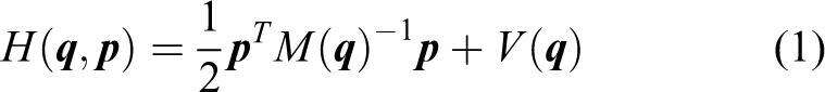
A brief review on the IDA-PBC method applied to the control of a class of underactuated mechanical systems is presented (see the work done by Ortega et al. 3 for further details). The procedure starts from the Hamiltonian description of the system by means of the total energy function (kinetic plus potential energies) given by
where

being

where

where

where

Furthermore, if Md is a positive definite in a neighborhood of

then
Compass-like biped robot
The simplest known biped robot is called CBR, which has two rigid legs joined by the hip that presents a stable gait without actuation in a determined slope, known as passive walking gait. 16 A schematic picture of the CBR is shown in Figure 1, and the description of the parameters is presented in Table 1.
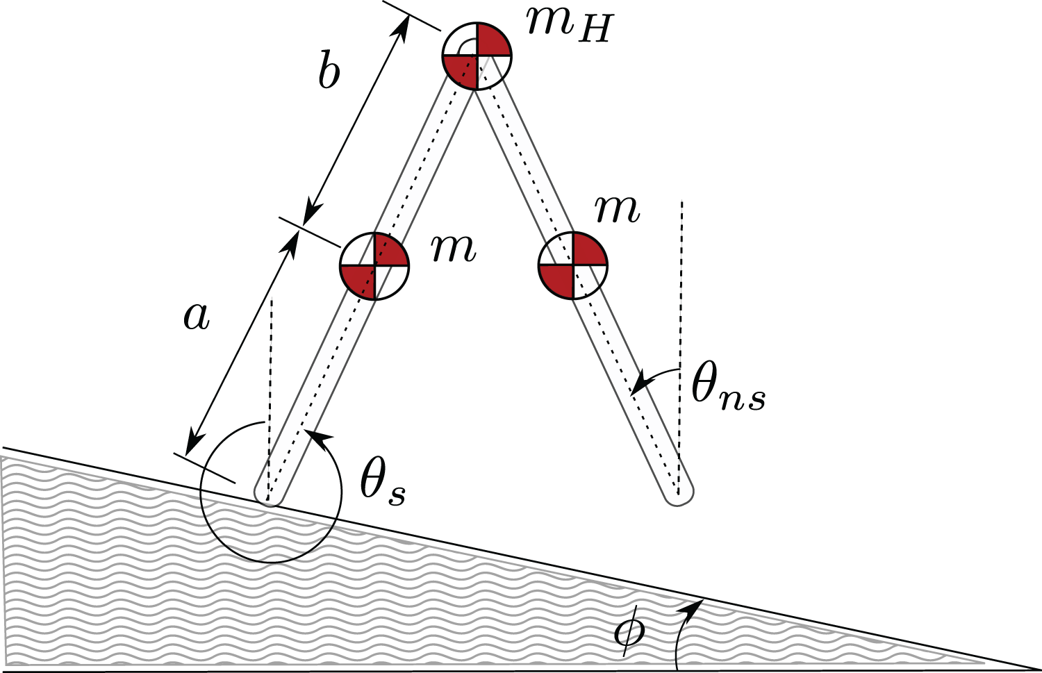
CBR diagram. CBR: compass-like biped robot.
CBR parameters.

CBR: compass-like biped robot.
The motion of the CBR is restricted to the sagittal plane, having a compass-like motion, that is the reason why this biped robot is identified in the literature by that name. The CBR configuration is defined as θs and θns which are the angular positions of the support and nonsupport legs, respectively, measured from the positive vertical axis. Also, it is taken into account φ as the slope inclination of the ground on which the biped robot walks. The gait is split into two phases: the balance phase and the foot impact as shown in Figure 2. The equations that describe this entire motion are presented next.

Walking gait phases of the CBR. (a) Balance phase and (b) foot impact. CBR: compass-like biped robot.
Balance phase
The behavior of the CBR during the balance phase is described by the EL equations (see 16 for further details) given for

where

Note that, for the case of the full-actuated system,
Foot impact
At the end of the balance phase, an impact with the ground is produced. The impact of the CBR foot with the ground is considered as an instantaneous change of the velocity and it is obtained by applying the angular momentum conservation law. In order to know when the impact is produced, it is useful to define the vertical distance from the nonsupport foot to the ground, which is given by (see Figure 1)

where the derivative from equation (10) with respect to time yields

An impact occurs when the next conditions are satisfied
16
:
yh = 0. The foot of the nonsupport leg is touching the ground.
When these conditions are satisfied, an instantaneous change of velocities is applied, 16 which is described as

where

with
So, meanwhile equation (12) takes into account the change of the angular velocities at the impact time, the roles of the support and nonsupport legs also change (they swap). This change of the angular positions θns and θs is described by

with
Equivalent dynamic model of the CBR
The design of the IDA-PBC for the CBR follows the strategy presented by Acosta et al. 6 for systems with underactuation degree one. A feature of the strategy in the study by Acosta et al. 6 is that the inertia matrix must depend only on the nonactuated coordinates, and according to equation (9), the M matrix of the CBR system depends on both joint coordinates θs and θns.
Therefore, a change of coordinates is proposed in order to achieve a suitable dynamic model of the CBR where the second joint (i.e. the hip) is the nonactuated one, such as the CBR dynamic model be similar to the Pendubot model shown in the study by Sandoval et al. 22 Thus, in the following, this model will be called Pendubot-like biped robot (PBR). This model can be expressed in a compact form as

where

PBR diagram. PBR: pendubot-like biped robot.
So, the matrices of equation (14) are defined as


and

Furthermore, according to the study by De-León-Gómez et al., 23 a relation between model (9) and (14) is given by (equivalence (21) is used for the case of full-actuated system)


where the relationship between the generalized coordinates

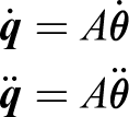
where A and
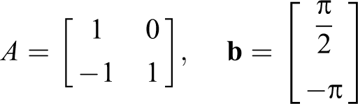
such as the time derivatives yield
Using the equivalences (18) to (21), it is possible to transform the PBR model (14) into the CBR model (9) and viceversa by making the corresponding operations (see the relationship of models reported by De-León-Gómez et al. 23 for further details). Therefore, the PBR dynamic model will be used to design an IDA-PBC and the CBR dynamic model will be used to carry out numerical simulations.
An IDA-PBC for the CBR
In this section, the design of an IDA-PBC for producing a stable limit cycle for the CBR is presented. Inspired by Holm and Spong, 20 where a controller based on the kinetic energy shaping using the CL method is proposed, our IDA-PBC also only shapes the kinetic energy by leaving unaltered the original potential energy of the system, that is, Vd = V. Then, the PBR dynamic model (14) is used to follow a similar procedure to that shown in the study by Sandoval et al. 22 to get an IDA-PBC.
Dynamic model
The Hamiltonian model of the PBR shown in Figure 3 can be described by equation (2) with the matrices


and the potential energy function

where the constants ci with i = 1, 2, …, 5 are defined as

For convenience of notation, the elements of the matrix M(q2) given in equation (22) are named as follows

IDA-PBC design
First, we define

such as
being

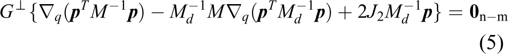
the first PDE (5) yields

where e2 is a base vector. Now, equation (29) can be expressed as

where uniquely has been assigned the symmetric part of the matrix

It is worth to remark that the matrix
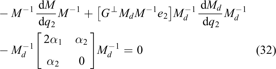
which pre-multiplying and post-multiplying by Md and defining

Before continuing, it is convenient to notice that until now, the strategy of design that we have followed seeks to ease the solution of Md in equation (5). In our case, the set of PDEs shown in equation (5) has been transformed into the set of differential equations in equation (33), which presents no obstacle in the solution of Md, because α1 and α2 are free. Now, we continue our design considering from the definition of the matrix Λ that


By taking into account (34) and (35) in equation (33), a set of algebraic equations given by
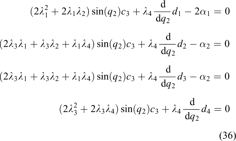
is obtained. Since d2 = d3 must be satisfied, just three equations are considered, and using equation (35) in equation (36), we have


On the other hand, from the second PDE (6), due to Vd = V, it results

where substituting V, we have

Then, it is necessary to find the values of the elements of matrix Λ that are solution of equations (37) to (40). By inspection, it is proposed λ3 = 0 and λ4 = 1, which are solution of equations (39) and (40). With this, we have

where


By solving these equations, we have that d2 = a2 and d3 = a3. Hence, until now the matrix Md is defined as

That is, it only remains to define the element d1. Then, proposing λ1 = k where k will be a free parameter strictly positive, we have from the definition of Λ that

Due to

where by solving for λ2, we get
and by substituting equation (47) into equation (45), finally Md yields

Positivity of matrix Md
In order to achieve that Md be definite positive, it must be fulfilled that d1 > 0 and


is satisfied, since
Matrix J2
Then, using equations (37) and (38) with λ3 = 0 and λ4 = 1, these equations can be reduced to

By solving equations (51) and (52) for α1 and α2, we have

where by substituting λ1 = k and λ2 from equation (47), we get

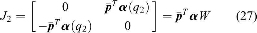
which are used to define the J2 matrix from equation (27), which is

with

being
Simulation results
The controller (7) with
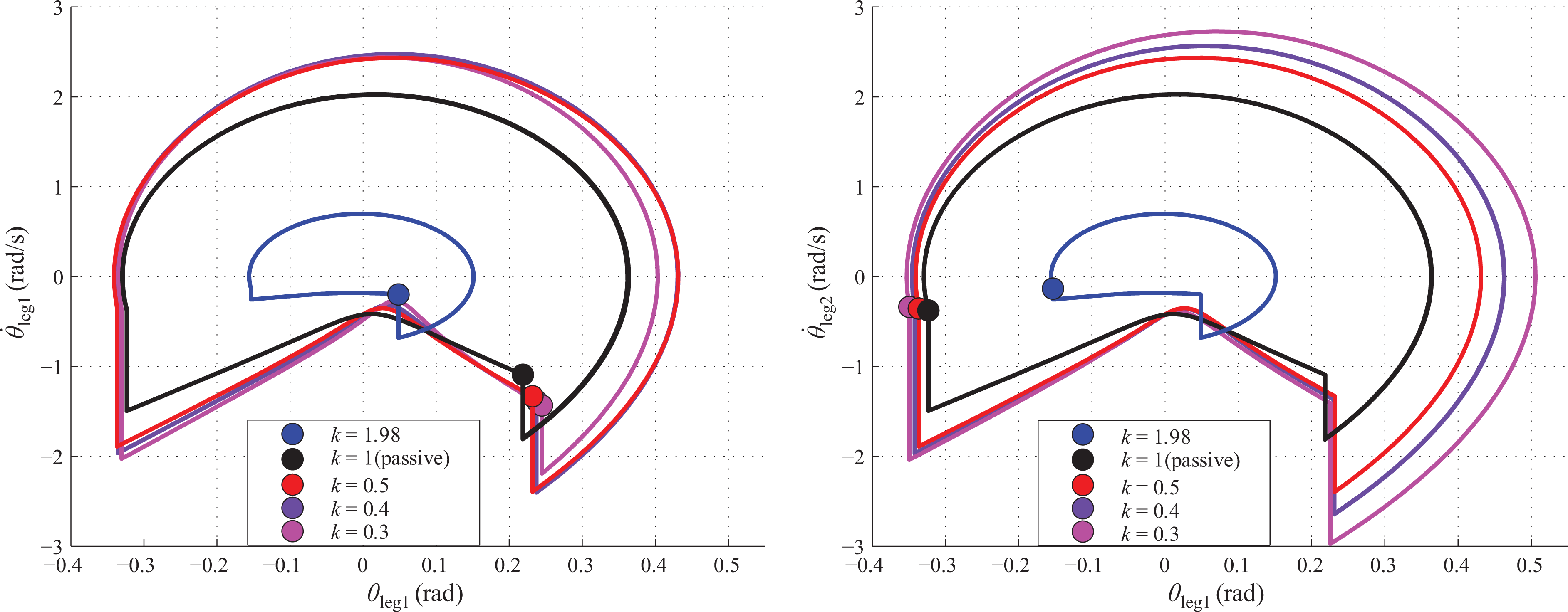
It could be noted, from equations (48) and (53), that with k = 1, the system is not modified and the dynamic model is still the same, since Md = M and J2 = 0, thereby a limit cycle is produced by an intrinsic property of the system, which represents a walking without actuation called passive walking gait. However, this limit cycle can be modified; namely, the gait of the robot can be changed, by varying k in our controller as shown in Figures 4 and 5. The phase diagram of both legs using coordinates of position

Limit cycles corresponding to different gaits of a CBR using the IDA-PBC (7) with equations (48) and (53). By varying k, the limit cycle is modified, while for k = 1, the limit cycle corresponds to the passive walking gait. Left and right figures show the evolution of the states using as generalized coordinates, the position θ and momentum p, for the leg one and leg two, respectively. CBR: compass-like biped robot; IDA-PBC: interconnection and damping assignment passivity-based control.
Gait modification of the CBR for different values of k with the IDA-PBC (7) with equations (48) and (53). Left and right figures show the initial condition for leg one and leg two, respectively, using as generalized coordinates the position θ and velocity
Let us remark that small changes in the gain k produce a big change in the limit cycle. In fact, our controller can produce very short steps at very slow velocities, as shown in Figures 5 and 6. However, these figures also show that it is not possible to perform very large step lengths since the walking of the robot becomes asymmetrical. It is observed that for k < 0.5, limit cycles of leg one and leg two are not identical (see Figure 5), and gait parameters T, S, and v, defined in Table 2, are different for each leg (see Figure 6). Table 2 shows the initial conditions for each limit cycle produced for each value of k and also the corresponding gait parameters of each walking gait.
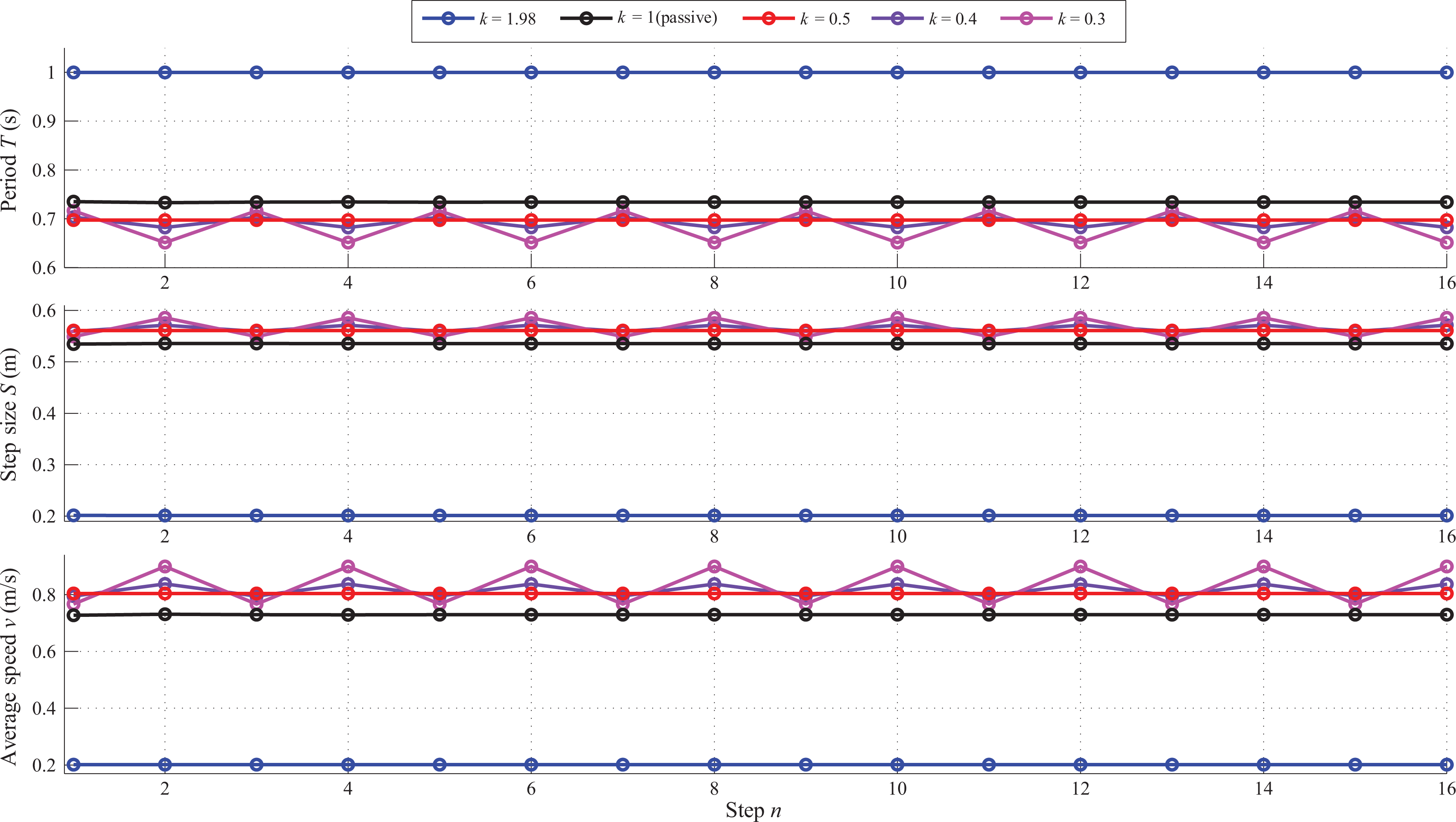
Gait parameters corresponding to each walking gait of the CBR for those values of k shown in Figure 5 with the IDA-PBC (7) with equations (48) and (53). CBR: compass-like biped robot; IDA-PBC: interconnection and damping assignment passivity-based control.
Initial conditions and gait parameters for each limit cycle of the CBR obtained with different values of the gain k in the IDA-PBC (7) with equations (48) and (53).

CBR: compass-like biped robot; IDA-PBC: interconnection and damping assignment passivity-based control. The bold values correspond to the passive walking gait.
Controlled Lagrangian
As mentioned before, the design of the IDA-PBC shown in “An IDA-PBC for the CBR” section is inspired in the energy-based controller reported in the study by Holm and Spong. 20 In order to compare both control laws, in this section, a very brief review is given. The CL control law is given by 20
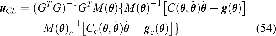
where M(

and

Gait modification of the CBR for different values of k with the CL control law (54). Left and right figures show the initial condition for leg one and leg two, respectively. CBR: compass-like biped robot; CL: controlled Lagrangian.

Gait parameters corresponding to each walking gait of the CBR for those values of k shown in Figure 7 with the CL control law (54). CBR: compass-like biped robot; CL: controlled Lagrangian.
Initial conditions and gait parameters for each limit cycle of the CBR obtained with different values of the gain k in the CL control law (54).

CBR: compass-like biped robot; CL: controlled Lagrangian. The bold values correspond to the passive walking gait.
Analysis and comparison
Before comparing the CL control law (54) and the IDA-PBC (7), let us recall the natural behavior of the passive walking gait. As we know, the natural passive gait of the CBR is not robust, that is, a small variation of the initial conditions affects the evolution of the states and it could turn them away from the limit cycle, that is, the basin of attraction is very small. 16 In other words, a little disturbance in the gait of the robot can make it fall. In order to introduce a perturbation on the initial conditions, a percentage of their current values is added as follows

where Pθ is the percentage added to both initial positions
The inclined slope is always 3° for all cases. The extreme values of the initial condition that the passive gait can handle are shown in Table 4 and plotted in Figure 9. The convergence to the limit cycle is slow but effective at these values.
Extreme initial conditions values for the passive gait, IDA-PBC (7), and CL control law (54).

CL: controlled Lagrangian; IDA-PBC: interconnection and damping assignment passivity-based control.

Four extreme initial conditions for the natural passive gait of the CBR, that is, without actuators. Initial conditions are marked with solid circle. Evolution of the states for leg one and leg two is shown in left and right figures, respectively. CBR: compass-like biped robot.
On the other hand, the energy-based controllers (the CL control law (54) and the IDA-PBC (7)) do not pretend to increase the basin of attraction of the robot but to change the limit cycle shape and thus the walking behavior. Nevertheless, it is interesting to test the basin of attraction using both controllers in order to know if they also improve or not this feature. Since both controllers produce different shaping of the limit cycle as shown previously (Figure 5 for IDA-PBC and Figure 7 for CL), two limit cycles that perform similar step lengths have been chosen in order to compare them. The two chosen cases are The limit cycle for the larger symmetrical step length that the IDA-PBC (7) with equations (48) and (53) can perform, that is, with k = 0.5. In counterpart, k = 1 has been chosen for the CL control law (54). As observed in Figure 10, both controllers produce a similar step length but with the IDA-PBC, the steps are faster. The limit cycles produced for both controllers are plotted in Figure 11, where it is shown the similitude in the limit cycle along the x-axis corresponding to the step length, but a larger limit cycle is produced by the IDA-PBC on y-axis corresponding to the velocity. The limit cycle for the smaller symmetrical step length that the CL control law (54) can perform, that is, with k = −7. In this case, a value of k = 1.8 has been chosen for the IDA-PBC (7). As depicted in Figure 12, both controllers produce a similar step length but with the CL, the steps are faster. The limit cycles produced for both controllers are plotted in Figure 13, where it is shown the similitude in the limit cycle along the x-axis corresponding to the step length, but a larger limit cycle is produced by the CL controller on y-axis corresponding to the velocity.
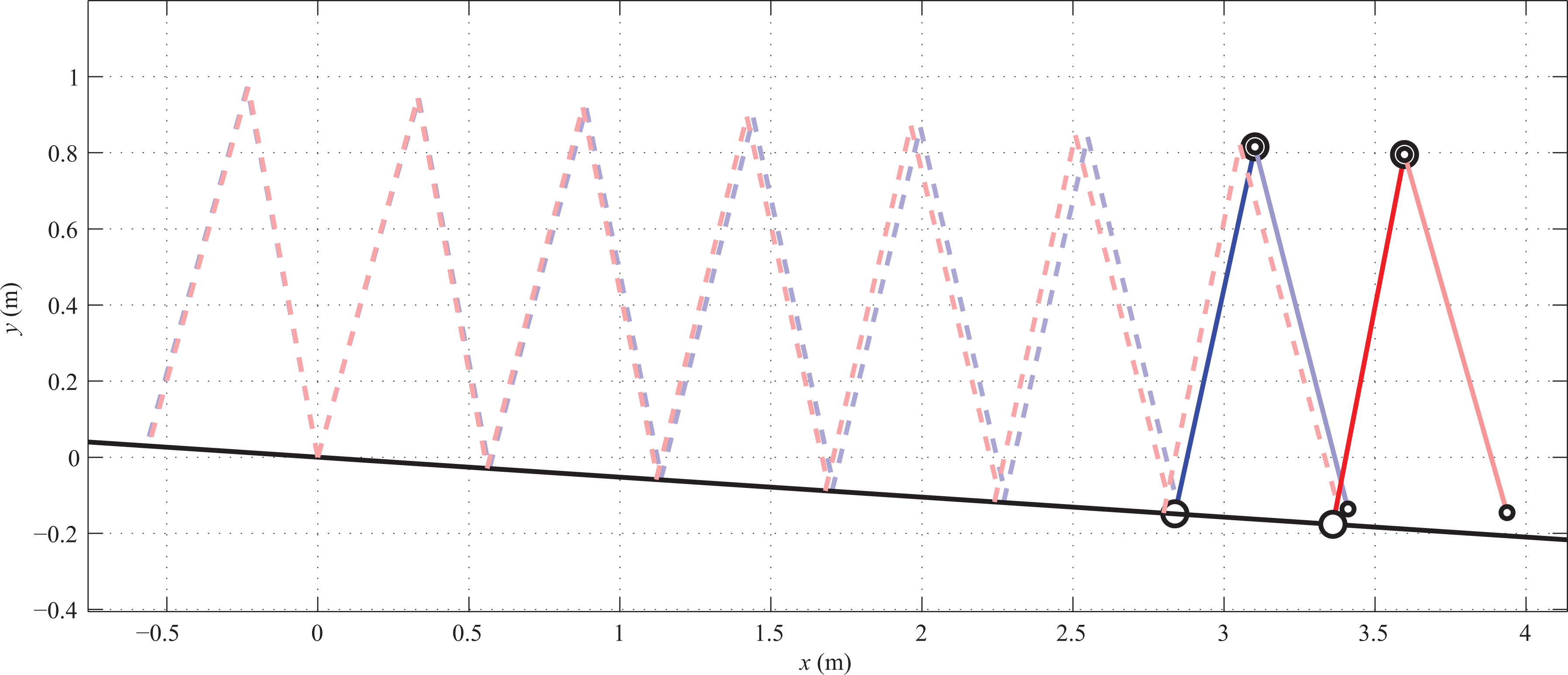
Five seconds of walking with a large step length of the CBR, using CL (in blue) or IDA-PBC (in red). IDA-PBC produces faster steps than CL. CBR: compass-like biped robot; CL: controlled Lagrangian; IDA-PBC: interconnection and damping assignment passivity-based control.
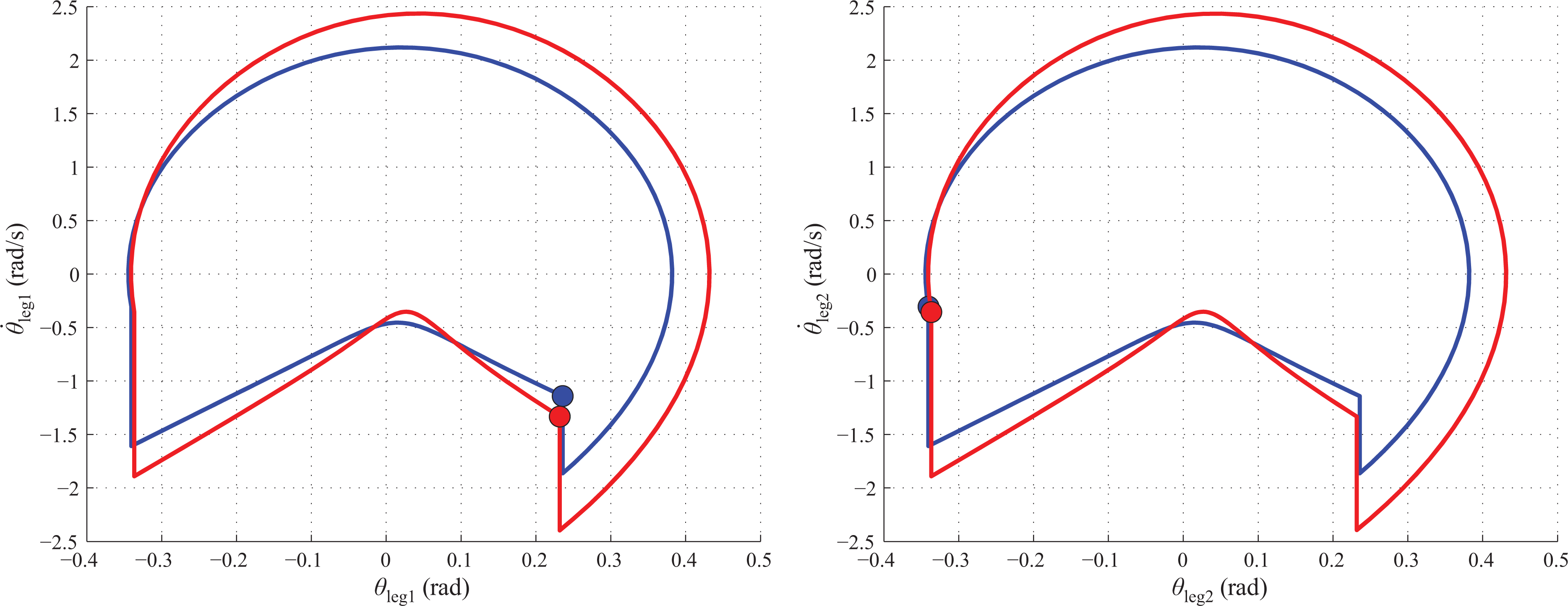
Similar limit cycles on the position (step length) for large gaits of the CBR using CL (in blue) or IDA-PBC (in red). Initial conditions are marked with solid circle. Evolution of the states for leg one and leg two is shown in left and right figures, respectively. CBR: compass-like biped robot; CL: controlled Lagrangian; IDA-PBC: interconnection and damping assignment passivity-based control.
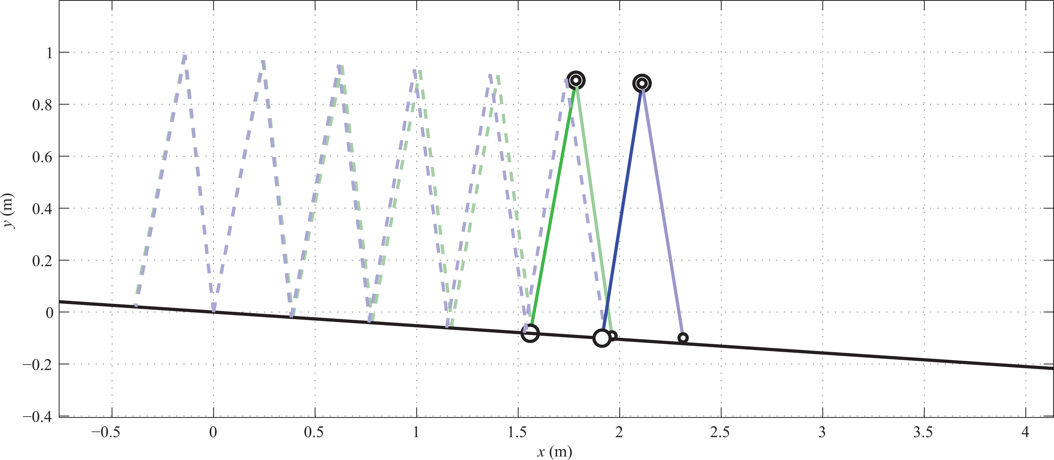
Five seconds of walking with a small step length of the CBR using CL (in blue) or IDA-PBC (in green). CL produces faster steps than IDA-PBC. CBR: compass-like biped robot; CL: controlled Lagrangian; IDA-PBC: interconnection and damping assignment passivity-based control.
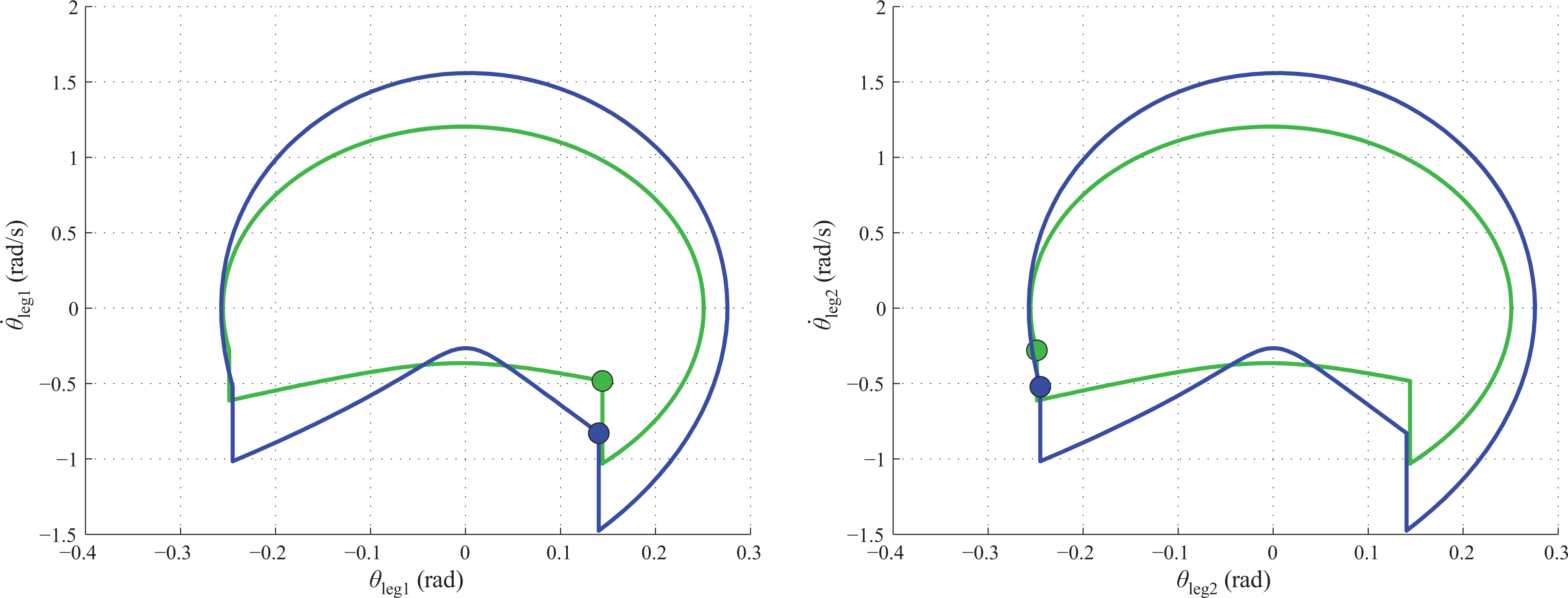
Similar limit cycles on the position (step length) for small gaits of the CBR using CL (in blue) or IDA-PBC (in green). Initial conditions are marked with solid circle. Evolution of the states for leg one and leg two is shown in left and right figures, respectively. CBR: compass-like biped robot; CL: controlled Lagrangian; IDA-PBC: interconnection and damping assignment passivity-based control.
Case 1. Large steps
Using (55), the initial condition for the CL (54) when k = 1 was changed. The maximum allowed perturbations are shown in Table 4 and plotted in Figure 14. As observed in Figure 14, the basin of attraction and evolution of the states are quite similar to the natural passive gait shown in Figure 9.

Large steps. Four extreme initial conditions for the walking gait of the CBR, with the CL control law (54) with k = 1. Initial conditions are marked with solid circle. Evolution of the states for leg one and leg two is shown in left and right figures, respectively. CBR: compass-like biped robot; CL: controlled Lagrangian.
On the other hand, the basin of attraction of the limit cycle produced by the IDA-PBC (7) is slightly reduced compared with that produced by the CL control law (54). Table 4 shows the maximum disturbances allowed for the IDA-PBC for k = 0.5 and the evolution of states is shown in Figure 15.

Large steps. Four extreme initial conditions for the walking gait of the CBR, with the IDA-PBC (7) with equations (48) and (53) with k = 0.5. Initial conditions are marked with solid circle. Evolution of the states for leg one and leg two is shown in left and right figures, respectively. CBR: compass-like biped robot; IDA-PBC: interconnection and damping assignment passivity-based control.
Case 2. Small steps
Using (55), the initial condition for the CL (54) when k = −7 was changed. The maximum allowed perturbations are shown in Table 4 and plotted in Figure 16. Again we can observe that the basin of attraction and evolution of the states are quite similar to the natural passive gait shown in Figure 9.
Small steps. Four extreme initial conditions for the walking gait of the CBR, with the CL control law (54) with k = −7. Initial conditions are marked with solid circle. Evolution of the states for leg one and leg two is shown in left and right figures, respectively. CBR: compass-like biped robot; CL: controlled Lagrangian.
In order to underline the fragility of the basin of attraction, a disturbance of

A little bit bigger disturbance than the maximum specified in Table 4 for the initial conditions makes robot fall. Here, a position disturbance
In contrast, the proposed IDA-PBC in equation (7) increases the basin of attraction when the walking gait is small, in this case with k = 1.8. As shown in Table 4 and plotted in Figure 18, the maximum perturbation allowed is really big, providing a less restrictive initial conditions to converge to the limit cycle. As we can see in Figure 18, the convergence of those extreme initial conditions is also faster than the convergence for the CL in Figure 16. In this case, the maximum disturbance in position of

Small steps. Four extreme initial conditions for the walking gait of the CBR, with the IDA-PBC (7) with equations (48) and (53) with k = 1.8. Initial conditions are marked with solid circle. Evolution of the states for leg one and leg two is shown in left and right figures, respectively. CBR: compass-like biped robot; IDA-PBC: interconnection and damping assignment passivity-based control.
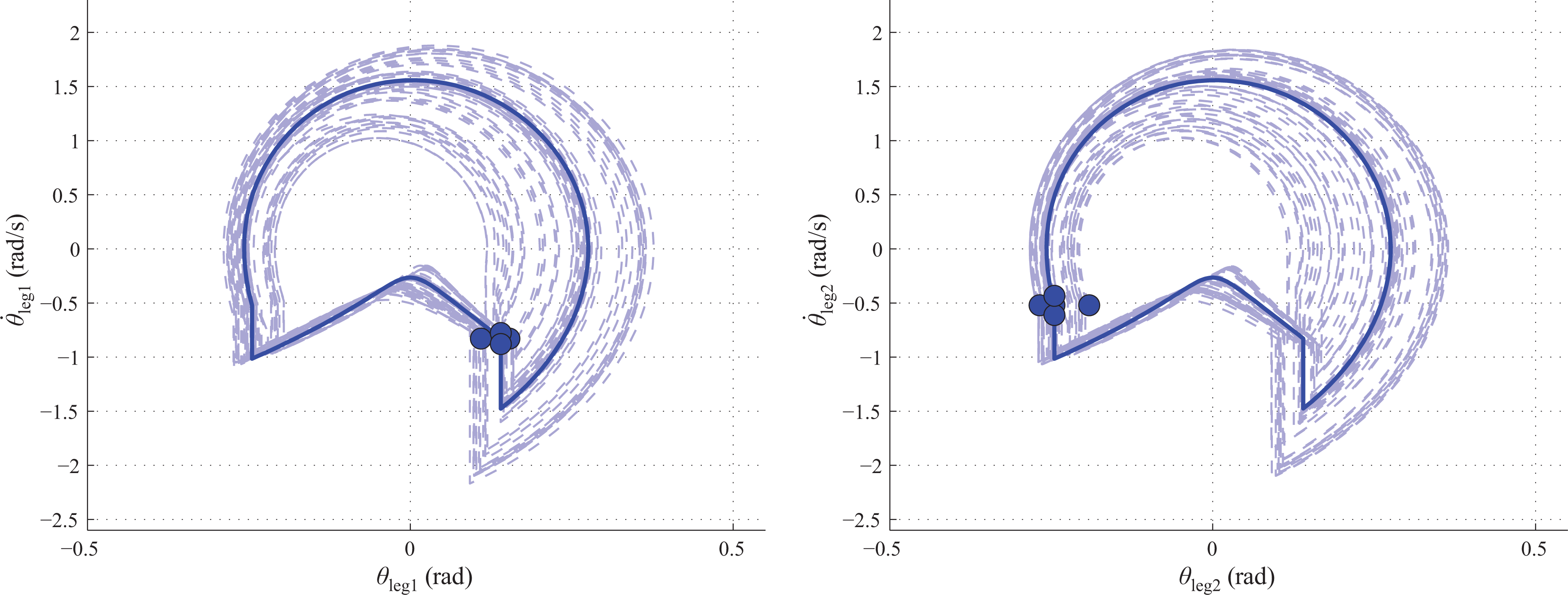
In order to test the robustness of the proposed IDA-PBC, several arbitrary initial conditions were chosen. The extreme initial conditions for the IDA-PBC (in green) and CL (in blue) for both legs are shown in Figure 19 (this figure is a close-up of initial conditions of Figures 16 and 18). Intuitively, we have chosen initial conditions inside of the extreme values. Table 5 shows the particular values for each initial condition. The convergence to the gait parameters T, S, and v defined for gain k = 1.8 in the IDA-PBC is observed in Figure 20, where it can be noticed that less than seven steps takes to converge to the gait parameters (i.e. to the limit cycle). Based on this results, we can conclude that the proposed IDA-PBC not only changes the walking behavior of the robot by shaping the limit cycle but also increases its robustness for slow steps.

Different initial conditions for the walking gait of the CBR, with the IDA-PBC (7) with equations (48) and (53) with k = 1.8. Blue circles are the extreme values of the initial conditions that CL can handle for the limit cycle with k = −7 (see Fig. 16). Green circles are the extreme values of the initial conditions that IDA-PBC can handle for the limit cycle with k = 1.8 (see Figure 18). Dark green color shows the initial condition in the limit cycle. Black, cyan, and magenta colors correspond to arbitrary initial conditions that converge to the limit cycle. Left and right figures show the initial condition for leg one and leg two, respectively. CBR: compass-like biped robot; CL: controlled Lagrangian; IDA-PBC: interconnection and damping assignment passivity-based control.
Arbitrary initial conditions to test robustness of IDA-PBC for k = 1.8 and gait parameters.

IDA-PBC: interconnection and damping assignment passivity-based control.

Convergence of the gait parameters, time period T, step length S, and velocity v, for the initial conditions of Figure 19 for the walking gait of the CBR, with the IDA-PBC (7) with equations (48) and (53) with k = 1.8. Dark green color shows the gait parameters of the limit cycle. Black, cyan, and magenta colors show the convergence to the gait parameters of the limit cycle. CBR: compass-like biped robot; IDA-PBC: interconnection and damping assignment passivity-based control.
Conclusions
This article has presented the design of an IDA-PBC in order to modify the natural walking gait of a CBR making possible to increase or reduce the step length and velocity simultaneously. A change of coordinates has been an important issue that gave us the possibility of using the method proposed by Acosta et al. 6 The simulation results have shown an enlargement or reduction of the limit cycle of the robot, which are similar to those obtained by the CL proposed by Holm and Spong. 20 However, the proposed IDA-PBC was obtained by following a simpler mathematical procedure than the CL control law. Furthermore, some advantages of the proposed control law (IDA-PBC) with respect to the CL control law have been evidenced by means of a numerical simulation study, such as the ability of performing very short step at slow velocities and the increase in the basin of attraction of the limit cycle for short steps, in contrast with the CL control law, which is very sensitive to small disturbances on the initial conditions for short and slow steps.
Footnotes
Declaration of conflicting interests
The author(s) declared no potential conflicts of interest with respect to the research, authorship, and/or publication of this article.
Funding
The author(s) disclosed receipt of the following financial support for the research, authorship and/or publication of this article: This work is partially supported by CONACyT under Grants no. 134534 and no. 166636 and by TecNM.