
Abstract
In this article, a prescribed performance-based adaptive neural network control scheme is proposed for an uncertain small-scale unmanned helicopter system subject to input saturations and output constraints. The radial basis function neural networks are employed to approximate system uncertainties. A nonlinear disturbance observer is developed to tackle input saturation. Meanwhile, the prescribed performance function is adopted to deal with output constraint. The closed-loop system stability is rigorously proved using Lyapunov synthesis. Finally, simulation results for unmanned helicopter system are presented to demonstrate the effectiveness of developed tracking control scheme using disturbance observer and radial basis function neural network.
Keywords
Introduction
Unmanned helicopters have received a considerable attention and extensive development in the recent years. 1 –3 Especially, the small-scale unmanned helicopter system with complex dynamics is sensitive to model uncertainty and external disturbance. 4 –7 To deal with this problem, multifarious robust controller design techniques have been developed. 8 –10 Chen et al. 11 and Choi and Yoo 12 investigated the controller design for the unmanned helicopter using disturbance observer and fuzzy approximator. Zhu and Huo 13 proposed a robust nonlinear adaptive backstepping method for the trajectory tracking control of the model-scaled unmanned helicopter with uncertain parameters. Lee and Tsai 14 and Zhu 15 proposed a nonlinear adaptive backstepping controller for a class of unmanned helicopters. Yue-Bang et al. 16 proposed an adaptive backstepping control for simplified unmanned helicopters with unmodeled dynamics and external disturbances. Visual positioning method has been widely used in unmanned helicopter flight control. 17 –22 In this article, to facilitate trajectory tracking controller design, a backstepping control strategy is adopted for the small-scale unmanned helicopter system. However, the aforementioned works did not involve the input and constraint problem for unmanned helicopter systems. Thus, in this article, we will develop an adaptive constrained control approach for the unmanned helicopter.
As we all known, neural network (NN) and nonlinear disturbance observer are two of the main solutions to improve the tracking performance and robustness of the closed-loop system. 23 –25 Considering the uncertain input delay and time-varying disturbance, Chen et al. 26 studied an NN-based robust control approach for the nonlinear systems. For the nonaffine nonlinear uncertain systems, Zouari et al. 27 developed an adaptive radial basis function NN (RBFNN) feedback control scheme. To guarantee the system with input saturation nonlinearities asymptotically stable, NN was incorporated into the variable structure control design framework in the study by Miao et al. 28 For a class of uncertain nonlinear systems in the presence of input saturations, a nonlinear disturbance observer-based dynamic surface control scheme was proposed by Cui et al. 29 In the study by Chen et al., 30 a recurrent wavelet NN-based nonlinear disturbance observer was designed, and the disturbance estimate was adopted into the controller design. As an effective method to deal with the external disturbance, disturbance observer has been attracted extensive attentions. 31,32 In this article, we will employ NN and disturbance observer to deal with the model uncertainty and external disturbance of the small unmanned helicopter, respectively.
Many previous works focus on the conventional helicopter flight control, in which the input/output constraints have been rarely considered. If the problem of input saturation is not considered in the controller design process, the tracking performance of closed-loop system will be severely degraded, what’s more, it may cause instability. Fortunately, several research methods on the control constraint problem have been reported in the literature. For example, anti-windup schemes were designed by Tong et al. 33 and Grimm et al. 34 To efficiently handle the input saturation, a positively invariant sets method was proposed by Cao et al. 35 and Richter. 36 Zhou et al. 32 studied an adaptive control law for the nonlinear systems subject to actuator saturation. Cao and Lin 37 developed an adaptive control algorithm for a class of minimum phase systems with input saturation. Zhong 38 employed an adaptive control method for the flexible spacecraft control system with input saturations. At the same time, there were some control methods proposed for the problem of output constraint. 39 Since the barrier Lyapunov function candidate was originally proposed by Ngo et al., it had been widely used for the nonlinear system control with output constraints. 40 By employing the barrier Lyapunov function, Ngo et al. 41 designed an adaptive neural control law to tackle the problem of control output constraint. Tee et al. 42 proposed an asymmetric time-varying barrier Lyapunov function-based controller to ensure constraint requirement for the nonlinear time-varying systems. The barrier Lyapunov function-based backstepping control scheme was proposed by Tee et al., 43 wherein constraints were presented in some or even all of the states. In the study by Tong et al., 44 for the constrained uncertain nonlinear systems, an indirect adaptive controller was investigated by employing fuzzy logic system and barrier Lyapunov function. Almost concurrently, by imposing explicitly prescribed bounds on both transient and steady-state tracking error performance, the prescribed performance control was proposed by Li et al. 45 Since then, prescribed performance control has attracted considerable research efforts. In the study by Bechlioulis and Rovithakis, 46 guaranteed prescribed performance-based adaptive tracking control method was investigated for the strict feedback systems. In the study by Bechlioulis and Rovithakis, 47 the prescribed performance was provided to position control for robotic manipulators. 48 The prescribed performance control approach was applied for the energy conversion systems in the study by Bechlioulis et al. 49 Although there exist some research results about input saturation and output constraint, the control problem for the small-scale unmanned helicopter system need to be further studied considering both input saturation and output constraint. In this article, nonlinear disturbance observer will be introduced to handle the input saturations, and prescribed performance function method will be introduced to handle the output constraints for the unmanned helicopters.
Motivated by above discussion and analysis, we will present an adaptive control law for the small-scale helicopter system subject to model uncertainty, unknown external disturbance, and input/output constraints.
The remainder of this article is organized as follows. In “Problem statement and preliminaries” section, we address the problem statement and present some preliminaries. Following that, “Controller design” section presents the design of adaptive neural tracking controller using the prescribed performance method and nonlinear disturbance observer. In “Simulation results” section, simulation studies of the proposed adaptive tracking controller for the small-scale helicopter system are presented. Some conclusion remarks are addressed in “Conclusion” section.
Problem statement and preliminaries
In this section, it is particularly aimed to briefly review the completed nonlinear dynamic model of unmanned helicopters and introduce some preliminary knowledge about NN and prescribed performance-based control method.
Helicopter model
The considered small-scale unmanned helicopter in this work is Trex-250. Moreover, the external disturbances are introduced by adding some aerodynamical additional forces and torques. The rigid-body dynamic equations of the small-scale unmanned helicopter are described in the form of 14
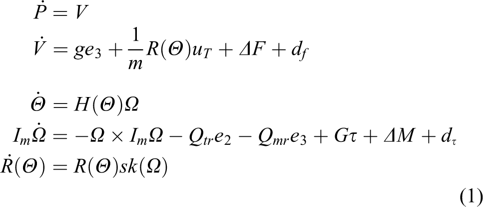
where P = [x, y, z] T is the position and V = [uv, vv, wv] T is the velocity; Θ = [ϕ, θ, ψ] T and Ω = [p, q, r] T are the attitude angle and angular rate, respectively. e3 = [0, 0, 1] T , g represents the gravitational acceleration, m ∈ R indicates the total mass, and Im ∈ R3×3 denotes the inertial moment matrix. Qmr and Qtr, respectively, denote the main rotor anti-torque and tail rotor anti-torque. G∈R3×3 is the control matrix related to the control moments. ΔF and ΔM, respectively, indicate the force and moment uncertainties, and df and dτ indicate the external disturbances. H(Θ) stands for the transformation matrix which can be represented as

Here, sk(Ω) indicates skew-symmetric matrix for the angular rate vector, and R(Θ) denotes the rotation matrix from body-fixed coordinate frame to inertial coordinate frame, which are derived as


where S(⋅) and C(⋅) indicate trigonometric functions sin(⋅) and cos(⋅), respectively. uT ∈ R3 and τ ∈ R3 denote acting forces and control torques on the helicopter, respectively. Furthermore, considering the input saturation, the acting forces can be described by

where
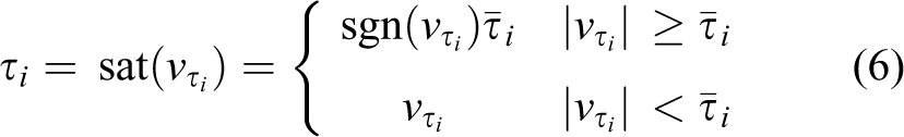
where
Neural networks
In recent literature of robust adaptive control, due to the inherent approximation capabilities of RBFNNs, they are mostly adopted as approximator for the unknown nonlinearities. Suppose that Δ(ω) : Rq → R represents an unknown and smooth nonlinear function, which can be approximated on the compact set Ω ⊆ Rp by a class of linearly parameterized RBFNNs 26

where ω = [ω1, ω2, …, ωq]
T
∈ Rq means the approximator input vector, S(ω) = [s1, s2, …, sp]
T
∈ Rp is the basis function,

where ε* represents the approximation error for special case:

where

where bi ∈ R and ci ∈ Rm are the width and center of the neural cell, respectively.
Prescribed performance function method
We know that one of the control objective is to deal with the output constraint, and the prescribed performance function method will be introduced in this article. Here, we recall some preliminary results and definitions which are necessary in the following design and analysis.
Definition 1
A smooth bounded function ρ(t) : R+ + {0} → R+ can be called as a performance function, when ρ(t) is decreasing,

where
To achieve the tracking performance (11), the error transformation method is introduced to transform constrained tracking errors into unconstrained signals, and the error transformation function is defined as 46

where ϖ is the new transformed error. The transformation function S(ϖ) is rigorously increasing, and it satisfies 47

To proceed with the design of the robust adaptive control for the small-scale helicopter system (1), we make the following assumptions.
Assumption 1
The desired trajectories Pd(t) and ψd(t) are the known bounded sufficiently smooth functions of time, with bounded and continuous first derivative.
Assumption 2
All state vectors are available for measurement.
Assumption 3
The roll angle ϕ satisfies inequality constraints −π/2 < ϕ < π/2, and the pitch angle θ satisfies inequality constraints −π/2 < θ < π/2. 14
Assumption 4
The uncertain dynamics ΔF and ΔM is bounded

where
Assumption 5
The external disturbance df and dτ are slowly varying variables, and
Assumption 6
The time derivations of saturation errors
Remark 1
For the practical unmanned helicopter systems, it is well known that the time derivations of ΔvT and Δvτ are always bounded when actuators are determined.
Lemma 1
For any bounded initial conditions, suppose that there exist a C1 positive definite and continuous Lyapunov function V(x) and two class K functions π1, π2 : Rn → R, satisfying
The objective of this article is to design a robust adaptive controller subject to input and output constraint for the small-scale helicopter system such that it can track desired trajectories Pd(t) and ψd(t).
Controller design
In this section, the prescribed performance-based robust adaptive control scheme will be developed for the uncertain helicopter system. As mentioned earlier, the disturbance observer and prescribed performance function method are adopted to deal with input saturation and output constraint, respectively. Firstly, choose one appropriate prescribed performance function and design the virtual control based on the new error transformation form in the initial step. Then, the control strategy is to find an immediate control in each step, in which the RBFNN weight update law and disturbance observer are considered. The detailed design procedure can be described in the following steps.
Step 1: The position tracking error is defined as

where Pd ∈ R3 is the reference position trajectory. A performance function ρi(t) is chosen as 46

where ρi∞, ρi0, and l are positive constants. The decreasing rate e−lt of ρi(t) denotes the desired convergence speed of δPi. The constant ρi∞ represents the maximum allowable amplitude of tracking error at the steady state. Therefore, by choosing appropriate performance function ρ i (t) and design parameters, the bounds of system output trajectory can be assigned.
An error transformation is defined as

where

In order to simplify the analysis, we define MPi and NPi as follows

Considering equations (18) and (19), we have

where MP = diag{MP1, MP2, MP3} and NP = [NP1, NP2, NP3] T .

where KP ∈ R3×3 is the constant positive definite matrices. Then, the time derivative of ϖP becomes

Choose the Lyapunov function candidate
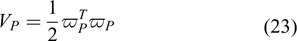
Substituting equation (22) into equation (23), we obtain

Step 2: Define the velocity tracking error item δV ∈ R3 as

Let γ = R3(Θ) ∈ R3×1, where R3(Θ) is the third column vector of the rotation matrix R(Θ). According to the definition of R(Θ), we know ∥γ∥ = 1. Define vT = −Tmre3, where

Since ΔF is unknown, using the RBFNN to approximate ΔF, we obtain

where pV > 0 is a design parameter. According to the definition of γ, we know ∥γ∥ = 1. Thus, define

The desired direction γ d and magnitude Tmr of the thrust vector can be designed as

where

The updating law of the RBFNN can be chosen as

where σV > 0 is a designed parameter, and ΓV ∈ R3×3 denotes the symmetric positive definite matrix. Meanwhile, the disturbance observer is chosen as follows

where ωV is the auxiliary variable, and

Considering equations (28) and (29), the time derivative of δV can be rewritten as

Choose the Lyapunov function candidate as

Let δγ = γ − γd and δγ = [δγ1, δγ2, δγ3] T . According to equation (29), we know that δγ3 = 0. Considering equations (24) and (34), we have

where δζ will be defined in equation (45), δV1,2 = [δV1, δV2] T indicates the first and second lines of δV, and δς will be designed in next step. Define ϑ1 = ϑT + ϑdf. Considering the following facts:

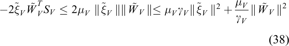
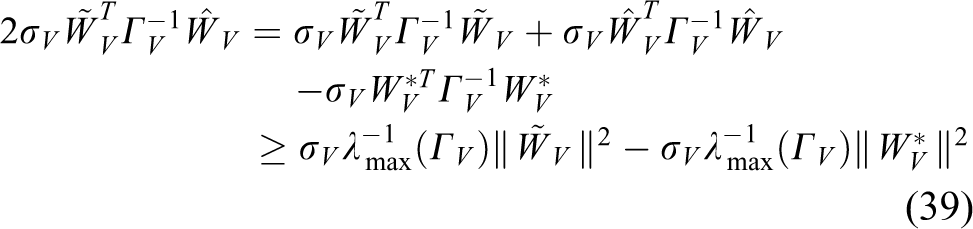
where μV > 0 and γV > 0 are the design parameters. Invoking equations (38) and (39), equation (36) can be rewritten as

Step 3: Define a new orientation variable ζ ∈ R2 as

According to the rotation matrix dynamic (3), we have

Then, the orientation dynamics can be obtained as

where

According to the definition of Z(Θ) and assumption 3, we can obtain |Z(Θ)| ≠ 0, where |Z(Θ)| indicates the polynomial of Z(Θ). Thus, |Z(Θ)| is reversible, and Z−1(Θ) denotes the inverse matrix of Z(Θ).
Using the ideal vector γ d , define ζd = [γd1, γd2] T , γdk, k = 1, 2 indicates the kth of γ k . Define the third error δζ ∈ R2 as

Choose the angular velocity virtual control as
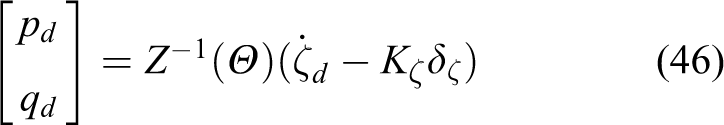
where Kζ ∈ R2×2 is the design matrix. Define δΩ1,2 = [p, q] T − [pd,qd] T . The reduced orientation error dynamics can be obtained as

Choose the Lyapunov function candidate as

Using equations (45) and (47), one obtains

Step 4: According to equation (1), the yaw dynamics is obtained

where H3(Θ) ∈ R1×3 indicates the third row of the matrix H(Θ). Define the yaw dynamics error δψ ∈ R as

where ψ d is the reference yaw signal. Invoking equations (50) and (51), we have

Similar to equation (17), we define the error transformation as follows
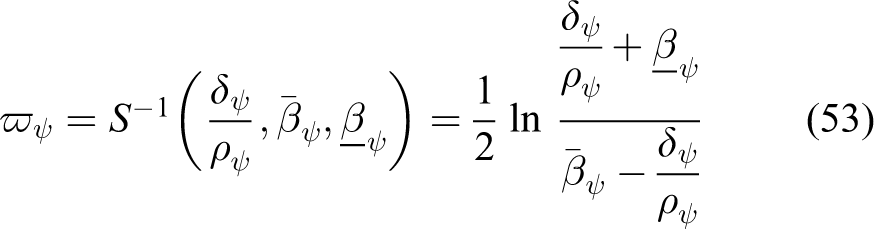
where
In order to simplify the analysis, we define Mψ and Nψ as follows

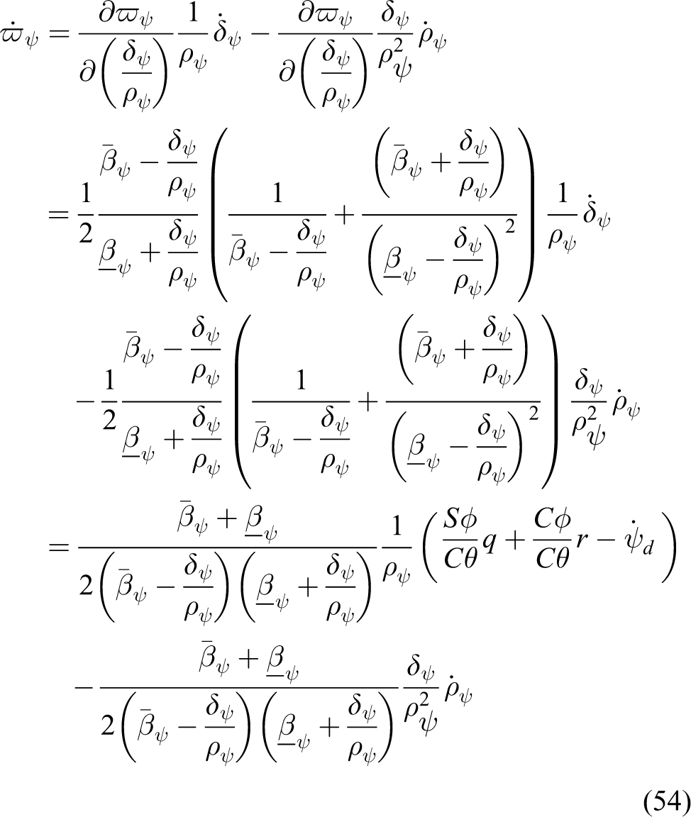
Designed the immediate control as

where Kψ > 0 is the designed constant. Choose the Lyapunov function candidate as

The time derivative of Vψ can be obtained as

Step 5: According to steps 3 and 4, we have obtained Ωd = [pd, qd, rd] T . Define the angular velocity error δΩ ∈ R3 as

Then we have
Since ΔM is unknown, using the RBFNN to approximate ΔM, we obtain

where pΩ > 0 is the design parameter. According to the definition of input saturation (6), the difference Δuτ between vτ and τ can be defined as Δuτ = τ − vτ. Define

Invoking equation (62), one can easily obtain the following ideal moment control
where KΩ ∈ R3×3 is the designed matrix.

where σΩ > 0, σΩ ∈ R is a designed parameter, and ΓΩ ∈ R3×3 represents the symmetric positive definite matrix. The disturbance observer is designed as follows

where ωΩ is the auxiliary variable, and

Choose the Lyapunov function candidate as

The time derivative of VΩ can be obtained as

Define ϑ2 = ϑτ + ϑdτ. Considering the following facts


where μΩ > 0 and γΩ > 0 are the design parameters. Invoking equations (69) to (71), equation (68) can be rewritten as
Theorem 1
Consider the Multiple-Input Multiple-Output (MIMO) nonlinear unmanned helicopter system (1) in the presence of input and output constraints. The adaptive laws of NNs are designed as equations (32) and (65). Disturbance observers are designed as equations (33) and (66). The adaptive prescribed performance control laws are designed as equations (21), (29), (46), (56), and (63). Then the closed-loop system is globally stable. Furthermore, by choosing appropriate design parameters, the trajectory tracking errors converge to an arbitrarily small neighborhood of the origin.
Proof
For considering the convergence of closed-loop state tracking errors and disturbance estimate errors, the Lyapunov function candidate for closed-loop control system can be chosen as

Differentiating VΣ and considering equations (24), (36), (49), (58), and (72), we obtain

where ρ and C are given by


Furthermore, the corresponding design parameters KP, KV, Kς, Kψ, KΩ, pV, μV, γV, pΩ, μΩ, γΩ, σV, ΓV, σΩ, and ΓΩ are chosen such that

According to equations (74) to (76), we have

From equation (78) and lemma 1, we know that the tracking errors δP, δV, δς, δψ, and δΩ; approximation errors
Simulation results
Now, we consider an uncertain nonlinear unmanned helicopter system, and the main parameters are given by Chen et al., 20 which is shown in Table 1.
Parameters for the small scale unmanned helicopter.

In order to verify the effectiveness of the proposed control method, two typical flight trajectories are proposed for the unmanned helicopter system. The reference trajectory is given by
Under the developed control scheme, the simulation results for unmanned helicopter are shown in Figures 1 to 8. Figures 1 to 3 show the position tracking results, where the solid lines indicate the real trajectories and the dashed lines indicate the desired trajectories. Obviously, the tracking performance of system is satisfactory; meanwhile, the tracking errors always be maintained between the prescribed performance bounds. Figures 4 to 6 show the velocities, attitude angles, and angle velocities of the unmanned helicopter, respectively. We observe that the states remain bounded. Figures 7 and 8 show the control moment and control thrust that do not exceed the limitation of inputs.

Tracking response of x.

Tracking response of y.

Tracking response of z.

The response of velocity V.
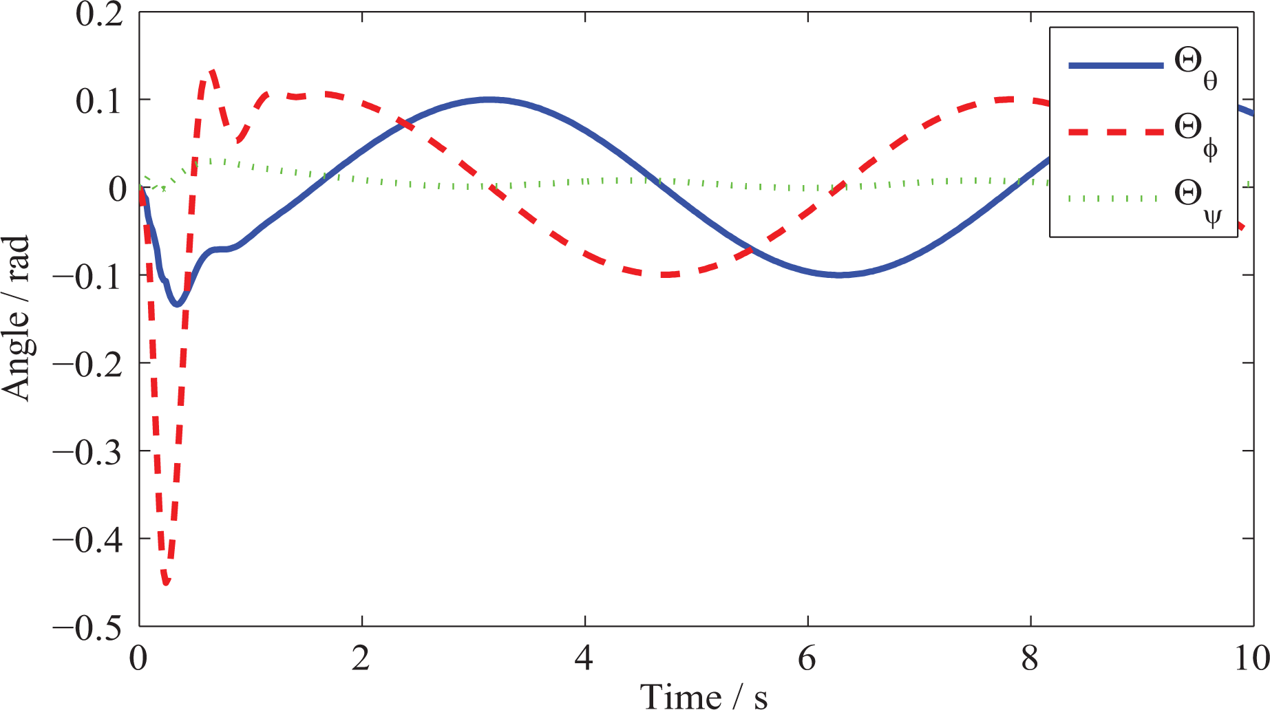
The response of angle Θ.
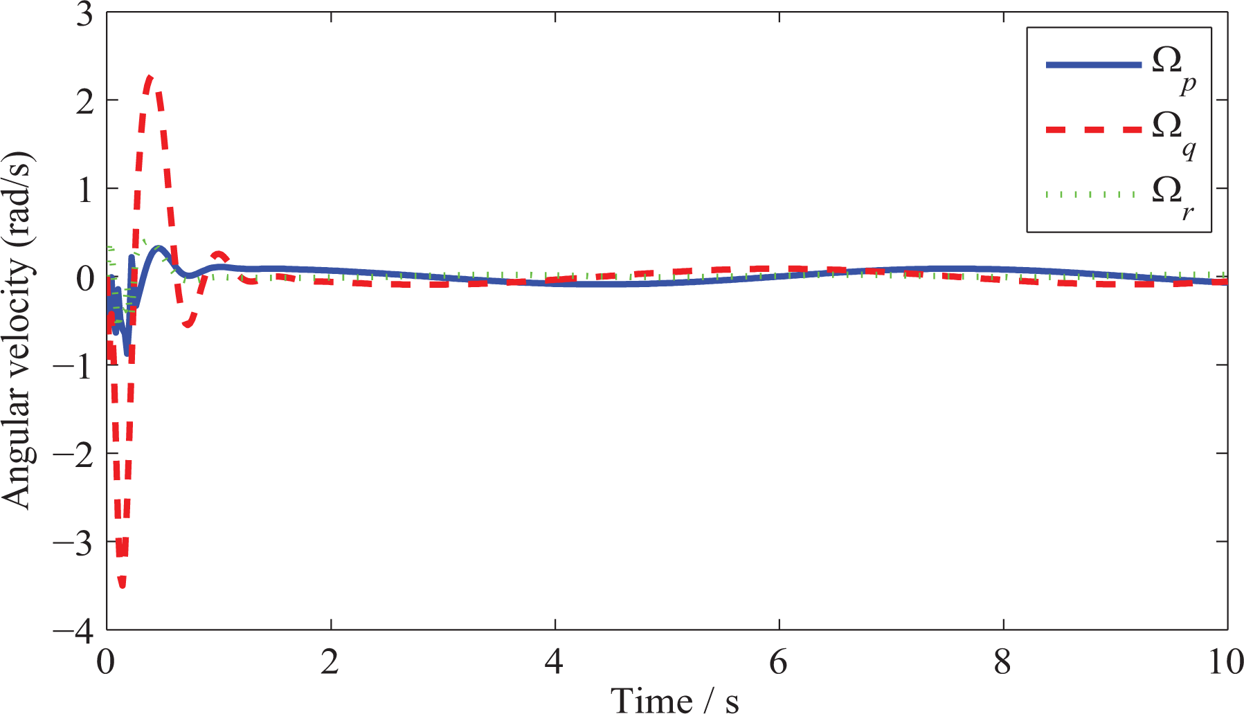
The response of angular velocity Ω.
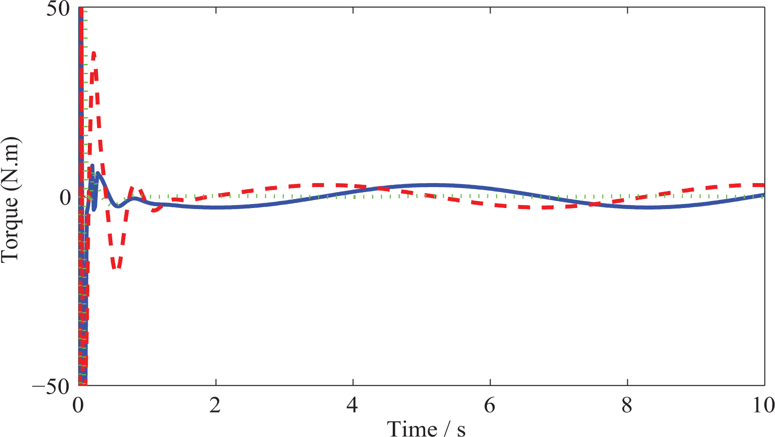
Control input moment τ.
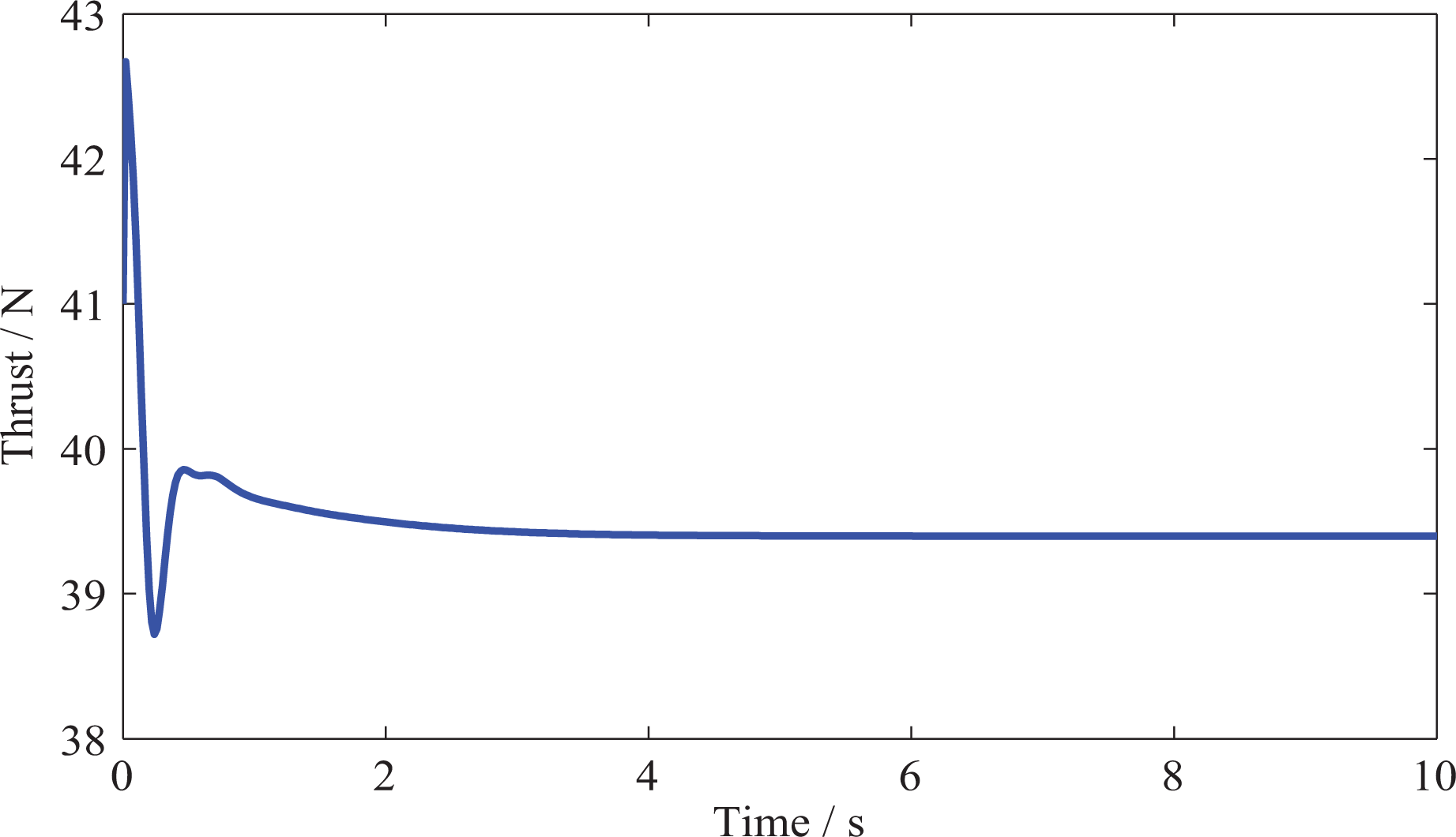
Control input thrust T.
It can be shown from these simulation results of the numerical example that the closed-loop system for the nonlinear helicopter system with input saturation and parametric uncertainties is asymptotically stable. Thus, the proposed robust control method is valid.
Conclusion
A robust adaptive neural control scheme has been presented to achieve trajectory tracking for a class of small-scaled unmanned helicopter in this article. Based on the adaptive backstepping control framework, nonlinear disturbance observer has been developed to compensate the input saturation and prescribed performance function method has been used to deal with the output constraint. Finally, simulation results have been given to illustrate tracking performance of the proposed robust adaptive control approach. The future research is going to consider solving the constrained control problem for unmanned helicopter with various external disturbances.
Footnotes
Declaration of conflicting interests
The author(s) declared no potential conflicts of interest with respect to the research, authorship, and/or publication of this article.
Funding
The author(s) disclosed receipt of the following financial support for the research, authorship, and/or publication of this article: This article was supported by National Natural Science Foundation of China (grant no 61573184, 61533008), Aeronautical Science Foundation of China (grant no 20165752049), and the Fundamental Research Funds for the Central Universities (grant no NE2016101).