
Abstract
In order to obtain the environment’s information, cooperative robots could need a lot of sensors. A possible solution to reduce the number of sensors might be the use of control–observer structures. In this article, we have designed a control algorithm by using a modified hybrid computed torque method based on the principle of orthogonalization, but in order to avoid the use of tachometers in the implementation, we are including a velocity observer. The stability proof is developed by using the theory of Lyapunov. Simulation of the proposed control structure compared with a well-known control structure via the performance index analysis is presented. Experimental tests are implemented with the control structure that has the best performance index.
Keywords
Introduction
Dexterity is one of the most desirable properties when a cooperative robot system is holding and manipulating an object. 1,2 In order to perform the task, it is necessary to define suitably the desired trajectories and forces to be applied by each end-effector. 3 Robot force control has been studied through decades. Raibert and Craig proposed the so-called hybrid position/force control by introducing a compliance selection matrix which distinguishes position control from force control components in Cartesian coordinates. 4,5 MaClamroch and Wang gave a proof for local stabilization by using linear feedback for set-point control when both constant target position and contact force are given to the manipulator. 6
On the other hand, Arimoto et al. proposed the principle of orthogonalization as an expanded notion of force/position control for robot manipulators under geometric constraints by separating position feedback signals from the force feedback ones by using projection matrices. 7 The main idea is to split position/velocity and force errors into two orthogonal spaces, one tangent to the physical constraint at the contact point and the other perpendicular to it. Yun-Hui et al. dealt with decentralized control of multiple manipulators in holonomic cooperation tasks based on the principle of orthogonalization. It should be noticed that a decentralized controller means that each robot is controlled by its own controller. In such a scheme, cooperations between the robots are realized by controlling their interactive forces. 8
Among many control techniques that can be found throughout the literature for cooperative systems, Hwang et al. studied grasp force for multi-slave tele-micromanipulation with a single master. 9 Similar to Hwang et al., unmanned surface vehicles have also attracted recent attention, that is, adaptive robust finite-time trajectory tracking control of fully actuated marine surface vehicles 10 ; direct adaptive fuzzy tracking control of marine vehicles with fully unknown parametric dynamics and uncertainties 11 ; adaptive robust online constructive fuzzy control of a complex surface vehicle system 12 ; and a novel extreme learning control framework of unmanned surface vehicles. 13 Murphey et al. considered environment uncertainties, concluding that these effects can be mitigated by using decentralized adaptive techniques. 14 Moreover, to improve the performance, Rahman and Ikeura took into account that weight perception due to inertia might be different from gravity when lifting an object. 15 More recently, Rugthum and Tao proposed an adaptive algorithm for cooperative systems in case of actuators’ failures, while guaranteeing asymptotic stability from the closed-loop errors. 16 In contrast, one of the most important rulings to deal with in position/force control of robots is the possible lack of tachometers and/or force sensors. Many solutions have been proposed in the literature. For instance, Huang and Tseng make use of nonlinear transformations for velocity/force observer design, 17 while Ohishi et al. applied H∞ techniques to avoid the use of force sensors. 18 Observers of the Luenberger type have also been employed, as shown in the literatures. 19,20 Martínez–Rosas et al. designed a linear velocity observer, avoiding the use of force sensors in an open-loop scheme. 21 Later, in 2008, Martínez-Rosas and Arteaga-Pérez improved this approach by including a force observer as well. 22
In this article, an innovative control law based on the hyperbolic tangent function with a velocity observer is proposed. The algorithm is an improvement over the control approach submitted in the literatures. 2,5 We compared the operation of both controllers by using the performance index.
This work is organized as follows: The second section presents the dynamic model of the system and their properties. The control structure and the observer are described in the third section. In the fourth section, experimental results are shown. Finally, conclusions are presented in the fifth section.
System model and properties
We consider a cooperative system consisting of l manipulators, each one with ni degrees of freedom and subject to mi
constraints, where ni
> mi
. Suppose the end-effector of the i-manipulator is in touch with an object, as shown in Figure 1. The surface is described by
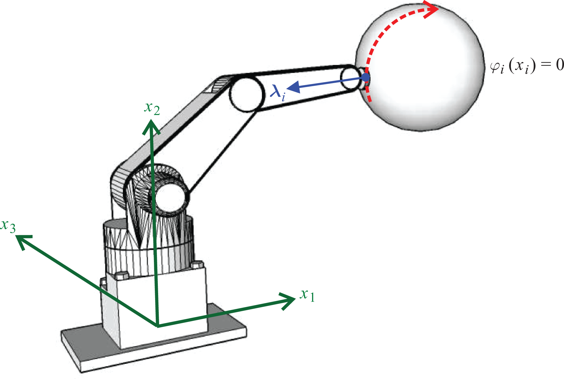
Hybrid control under a geometric constraint.

where

and which maps a vector onto the normal plane to the tangent plane that arises at the contact point. 2,5 This relationship means that homogeneous constraints are being considered. 2,5
Assuming for simplicity that all robots have got revolute joints, we can establish the following properties:

where
Remark 1
In workspace coordinates, constraint (2) becomes

and equivalently

with

In Figure 2(a), the case for a large tracking error is shown, while in Figure 2(b), it can be seen that

Plane tangent to the surface (tracking error). (a) Large tracking error and (b) small tracking error.

where

This means that a local stability analysis can be performed in a small enough region around


hold for a small enough error
In order to design the control-observer scheme, the following assumption is established. 21
Assumption 1
The contact between the object and each end-effector is firm, and it is made at one single point, as shown in Figure 1. This means that the relative movement between the surfaces does not exist and that the robots of the cooperative system satisfy the constraint
It should be noticed that assumption 1 is made for simplicity, but in practice, the control law must guarantee a firm contact with the object just by pushing it.
Control and observer design
In order to design the control law, based on the literatures 2,5 we consider the following auxiliary variables:


where
The nominal reference signal is defined as

where

where
By computing the derivative of equation (20), we obtain

where

with ajk
elements of
Based on equation (23), we define

where

where

where

where

Proposed controller
The control law is given by

where
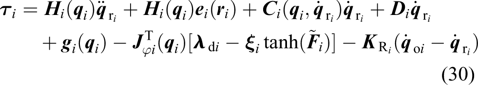
By applying the proposed control given in equation (30) into the dynamic model described in equation (1), considering the fact that

Taking into account property 3, we have

By substituting equation (32) in equation (31), we get the closed-loop error dynamics as

where

From (33), we obtain

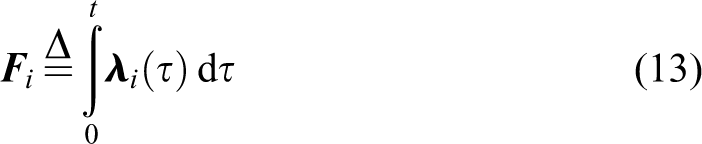
Observer definition
We propose the following observer:


where
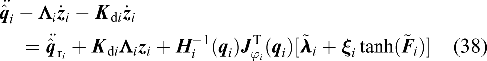
By substituting equation (27) into equation (38), we obtain

or
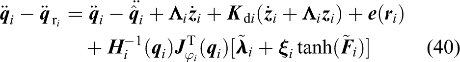
By considering equations (16), (17), and (18), we can rewrite equation (40) after equation (35) as follows:

Finally, we obtain the following closed-loop dynamics for the observer error

with

For the dynamic error system described by equations (12), (33), and (42), the state is defined as follows:

Consider now the following lemma:
Lemma 1
Assume that

where
Proof: It is rather obvious that

so that we can conclude that both
Note that for any
Remark 2
The region
Theorem 1
Consider the closed-loop dynamics (12), (33), and (42) formed by the cooperative system described in equation (1), the control law in equation (29), and the observer defined in equations (36) and (37), for i = 1,…,l. Assume that
The proof of theorem 1 is given in the Appendix 1, where a proper region of attraction is found.
Remark 3
The result of theorem 1 is only local within a possible (very) small region
Simulation and experimental results
In order to test the theory presented in the previous section, we have done some simulations and some experimental tests. The simulations were performed to compare the control structure proposed in the literatures, 2,5 and the control structure presented throughout this article. The experiments were carried out with the control structure that had a better performance according to the performance index analysis.
System description
The cooperative system consists of two industrial robots from CRS robotics (Figure 3). Robots are the CRS-A255 (5 DOF) and the CRS-A465 (6 DOF). It should be noticed that only the first three joints of each robot are used, while the remaining joints are mechanically braked. Each joint is driven by a DC motor with optical encoders, whose dynamics have been taken into account for control-observer implementation as explained by Gudiño Lau and Arteaga-Pérez. 23 The system’s framework is at A465 robot’s base. Both manipulators get a crash protection device on the end-effector, and a force sensor installed on it. Each end-effector is an interchangeably multi-tool, and it is set on the sensor. The experiments were performed on a personal computer with a Pentium IV 1.4 GHz processor with two PCI-FlexMotion-6C boards from National Instruments. The sampling time is 9 ms. The controllers are programmed in LabWindows/CVI software from National Instruments. The object is a cube of white melamine about 0.400 kg. The cube’s dimensions are 0.15 × 0.15 × 0.311 m3.

Cooperative system.
Simulation results
The task is to pick up an object with a desired force and move it into a plane. The corresponding constraints given in Cartesian coordinates are simply described by

where
It should be noticed that any desired trajectory should be chosen in order to fulfill the system’s constraints, and in this way, it is also easy enough to get a zero initial error whenever the initial velocities are null. For the simulation, it is then proposed


where ω(t) is a fifth-order polynomial designed to satisfy ω(t
i) = 0 and ω(t
f) = 2π for an initial time ti
and a final time t
f. In this way, the robots will make a circle in the yz plane. Inverse kinematics of the manipulators are used to compute
Control and observer parameters.

On the other hand, the main modification on the control law is the inclusion of the function

Position errors in Cartesian coordinates
On the other hand, in Figure 5(a) and (b), the effect of the new force control term on the system performance can be appreciated. The corresponding force errors are shown in Figure 6(a) and (b), where the improvement can be seen more easily.

Force tracking.
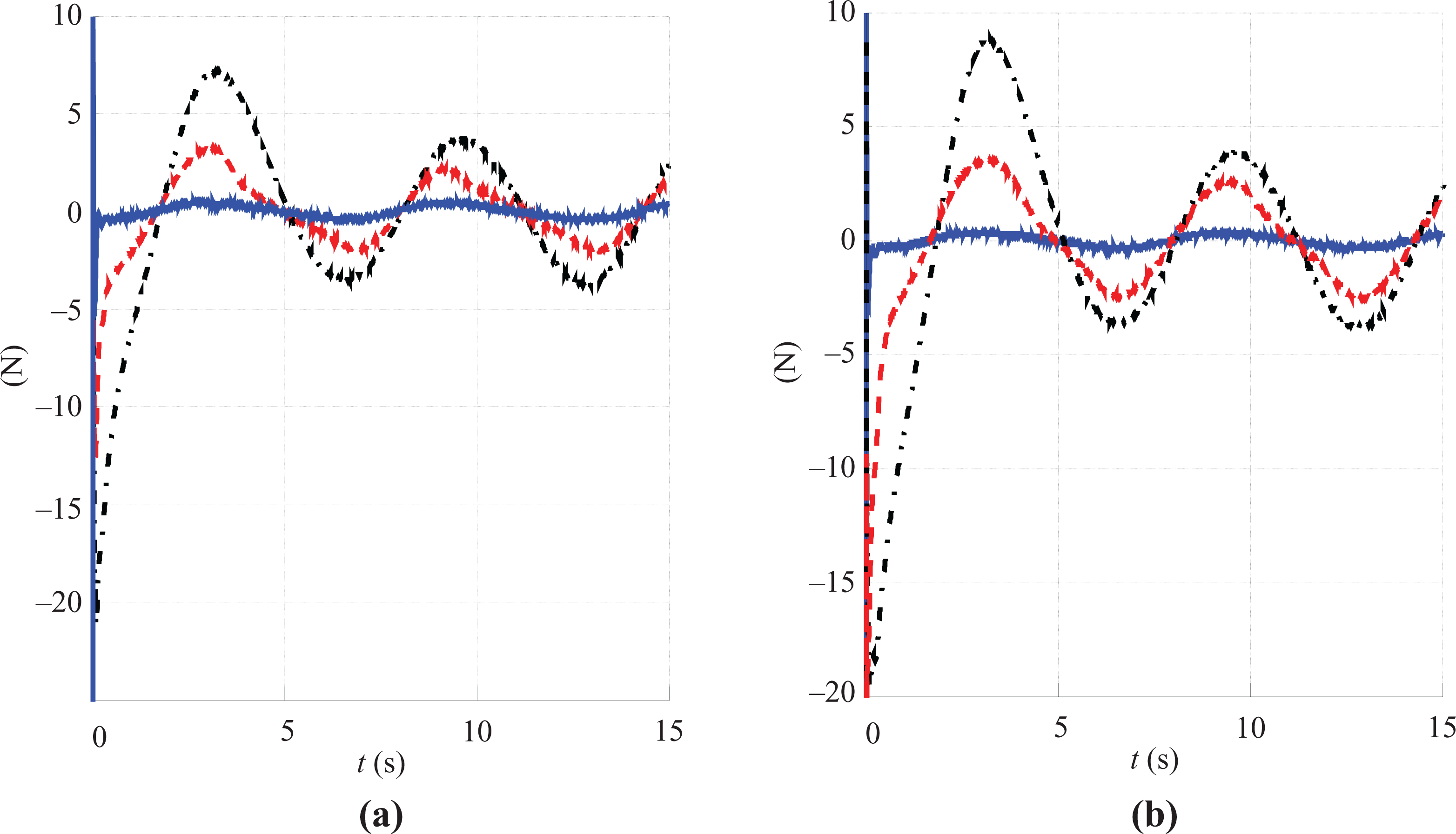
Force error.
Performance index
Robot manipulators are complex mechanical systems due to nonlinear and multivariable nature of their dynamic behavior. For this reason, in the robotics community, there are no well-established criteria for proper evaluation of the controllers. However, from a practical point of view, comparing the performance of the controllers using standard scalar value of
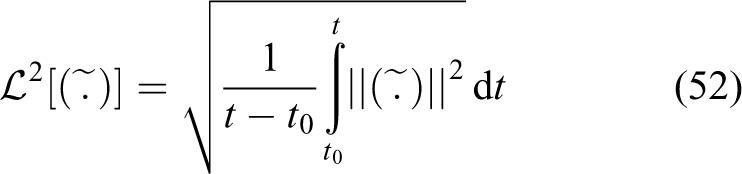
where

Performance index. (a) Position
Experimental results
We conducted experiments by using the control structure with the best performance index. In this case, the proposed control structure with
Experimental parameters.
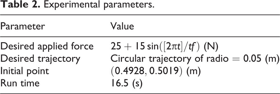
We can see in Figure 8 that the cooperative system follows the desired trajectory successfully. Furthermore, in Figure 9, we can see that both robots apply the right desired force on the object.

Trajectories.

Forces (applied, desired, and error).
The position errors in Cartesian coordinate are shown in Figures 10 and 11.

Position errors in Cartesian coordinate (robot A255).

Position errors in Cartesian coordinate (robot A465).
Since we proposed a velocity observer, and this was used in the design of control, then its behavior is presented in Figures 12 and 13.

Velocity observer (robot A255).

Velocity observer (robot A465).
Conclusions
The force and position tracking control without velocity measurements in cooperative systems formed by two robot manipulators holding an object is addressed in this work. The control law is a decentralized approach, which considers constrained movement directions in order to omit to know the dynamics of the object. It is assumed that the robot’s dynamics are known and that contact forces are measurable using a force sensor at the end-effector. In order to reduce the number of sensors used in a cooperative system, no velocity measurements are made, instead a velocity observer is proposed in order to obtain the information. The proposed scheme is based on the structure defined in the literatures, 2,5 with consideration to improve the force term. We focus on the term of force because the main objective is to hold a body firmly without breaking and follow a trajectory, for this reason the proposed control structure enhances the force term by using the hyperbolic tangent function. This modification improves performance in the force applied to hold the object and track the desired trajectory without dropping the body. By simulations, it is shown that force performance can be improved without decreasing position tracking. The results have been compared with the original algorithm, and the performance improvement is clear. Experimental results show the robustness of the proposed approach whenever robot model parameters are uncertain.
It is worth mentioning that the proposed solution is based on the properties of the hyperbolic tangent function, which is a real function, saturated, bijective in the condominium, odd, and strictly increasing.
Future work
Future work is to estimate the mass of the manipulated object and automatically adjust the force applied to avoid damaging the object.
Footnotes
Acknowledgments
The authors thank the DGAPA-UNAM under grants PAPIIT 116314 and 114617, the PRODEP (PROMEP) under the scholarship BUAP-811, and the Cátedra Especial Ángel Borja Osorno 2014.
Declaration of conflicting interests
The author(s) declared no potential conflicts of interest with respect to the research, authorship, and/or publication of this article.
Funding
The author(s) disclosed receipt of the following financial support for the research, authorship and/or publication of this article: The authors thank the financial support for the research and publication of this article to DGAPA-UNAM under grants PAPIIT 116314 and 114617, the PRODEP (PROMEP) under the scholarship BUAP-811, and the Cátedra Especial Ángel Borja Osorno 2014.
Appendix 1
The proof of theorem 1 is local and is valid for
After lemma 1, it is clear that
where
where
It is easy to see that
where
By calculating the derivative of equation (1E), we obtain
where
Substituting equations (33) and (42) into (1F), we have
After property 2, equation (1G) becomes
On the other hand, by using property 4, from equation (21), we obtain
Since
Substituting (1J) in (1H), we have
At this point, it is important to recall that the analysis is valid only in the region
where
By taking into account equations (34), (43), (1L)
to (1O),
Now we define
where δ1i , δ2i , and δ3i are positive constants. Then, we obtain
Clearly,
This can be shown rather straightforward. First of all, recall that by definition
exists for each subsystem
where