Sage Journals: Discover world-class research

Abstract

Future rover missions will be enhanced with the opportunistic search of salient targets during the planetary traverse phase. An essential component of the search is the locating and tracking of targets at the camera control level. The rover visual system must be able to follow quantified information gradients for smooth tracking in the visual field with limited information from images and delayed positional feedback caused by long communication delays inherent in planetary exploration. We propose a control algorithm based on vestibulo-ocular reflexes employed by the human cerebellum. The controller uses a feedback error learning model, which is able to track targets by compensating for the rover motion at the pan–tilt using a network trained prediction of the pan–tilt dynamics. The feedforward controller proved capable in tracking objects in the visual field as was demonstrated in both simulation and on the Barrett WAM.

Keywords

Feedforward control manipulators

Introduction

Planetary mission objectives are selected using NASA’s Follow the Water strategy, choosing scientific targets contingent on geographical indicators for past or present hydrological processes.^1,2 The resulting rock formations divulge volcanic activity, tectonic actions, and characterize past and current climates.³

Rover missions occur in two phases: a traverse phase and a scientific phase. The rover travels across the planet surface during the traverse phase until it reaches a preselected location where it then carries out the scientific phase in accordance with goals of the mission. The traverse consists of intervals in which the rover images the surrounding area, generates a map of obstacles, and designs a path through the imaged section. Future rover missions will be enhanced through the opportunistic search for new salient targets during this phase, which will require some form of active vision.

Active vision is a paradigm that suggests that the integration of controlled actuation may convert a nonlinear and unstable problem from passive observer to a stable solution for an active observer using multiple information sources.^4,5 Its use in the future will reduce the computational requirements and resources used in vision algorithms by focusing the processing on relevant concentrated areas of the visual field. This will require capabilities to allow the sensory instruments to track targets in both the real world and the sensor output. The real-world tracking occurs at the pan–tilt camera mount and needs to ensure the camera is viewing targets as the rover moves. Current tracking techniques track targets at the image processing level and use proportional-integral-derivative (PID) control laws to move the camera according to how the feature has moved in consecutive images. Since feedback signals in space applications are slow, this form of tracking quickly becomes unfeasible for rapid corrective motions, and therefore, such a controller will be without image feedback and will need to suffice with delayed positional feedback. These algorithms can also be computationally extensive, requiring simpler techniques to be used. Mass is another constraint in these missions, meaning hardware solutions are not viable.

A similarly constrained system occurs in the human body and is solved using the vestibulo-ocular reflex (VOR). VOR uses feedback from the vestibular system and the neck muscles as well as a predictive feedforward correction. The predictive component is trained to estimate the feedback error and compensate for it in the dynamics. We propose a controller that tracks objects in the visual field during the traverse phase of rover missions using a feedforward reactive controller similar to the visual reflex VOR. This will act as the front end to the application of active vision in rovers.

Background

The VORs maintain eye fixation during head rotations by counterrotating the eyes with typically unity gain and very low latency. Since feedback signals in the body travel slowly, the cerebellum, which is where the control center for VOR, uses a feedforward component to allow stable tracking. The fashion that the cerebellum controls VOR and other body motions is not well understood. Early theoretical models of the cerebellum were derived by Marr⁶ and Albus,^7,8 inspired by the work done by Braitenberg and Atwood⁹ and Eccles et al.¹⁰ Barto et al. showed that similar learning network models can be used to solve a problem like the cart and pendulum.¹¹ Albus proposed an alternative cerebellar controller called cerebellar model arithmetic computer (CMAC), later used by Miller to control 5-degree of freedom (DOF) manipulators.^12,13 Li and Leong applied the CMAC controller to a 5-DOF redundant manipulator to solve the inverse kinematic problem,¹⁴ as opposed to the control problem. Miall et al.¹⁵ and Miall and Wolpert¹⁶ proposed a version of the cerebellum in which it functions as a Smith predictor. The Smith predictor is designed for use in systems with pure time delay through the addition of a feedback loop with a delay model to predict the outcome of the time-delayed feedback.

Paulin et al. on the other hand have theorized the cerebellum as a fundamentally simple sensory processing organ.¹⁷ As such, he viewed the cerebellum as an analogue to either a Bayesian state estimator¹⁸ or Kalman filter.^19,20 This theory breaks what would normally be extended smooth motions with many DOF into smaller subsections. It would also suggest that models of the cerebellum could be derived from adaptive arrays.²¹

Kawato later proposed a feedback error learning (FEL) model of the cerebellum.^22
–24 The FEL model proposes that the cerebellum learns actual internal models of the proprioskeleto-muscular structure as well as the environment to be used in optimal control. Kawato and Gomi also proposed a generalized model of the cerebellum for each of its subsections. It differs from the Smith predictor in that the FEL model predicts the true model, where the Smith predictor predicts the error. Both cases reduce the dependency on delayed feedback.

The FEL model has been used in a few robotic applications. Miyamoto et al. used the model for trajectory control of a 3-DOF Programmable Universal Manipulation Arm (PUMA) manipulator²⁵ and Katayama and Kawato applied the controller to a 5-DOF rubber-actuator-arm.²⁶ Shibata and Schaal later applied the FEL to a humanoid robot face to emulate the VOR using a recursive least squares training law.²⁷ Some current investigations focus on using different feedback learning algorithms to optimize the process,²⁸ testing different network structures,²⁹ and applying the FEL model to adaptive control.³⁰ The natural progression is to integrate forward Smith predictor model with the learned internal model. Wolpert et al. proposed such a structure for the cerebellum; however, since the internal model greatly reduces the need for feedback, the structure did not result in a great improvement over the simpler internal model proposed by Wolpert et al.³¹ Attempts have been made to create a pan–tilt visual tracking algorithms with some feedforward control. Gilbert used adaptive statistical clustering and projection-based classification algorithms to identify and track objects in the visual field.³²

Corke and Goods proposed a visual servoing controller using a Kalman filter to approximate the motion of a moving target,³³ which was able to track better than using PI control alone. Chaumette and Santos proposed a similar control scheme using a Kalman filter-based estimation of the moving target.³⁴ Kobayashi and Shibata proposed a method where the target’s position is estimated with a technique based on triangulation on stereo vision system which again allows for the tracking of moving objects.³⁵ In these cases, the focus was on predicting the motion of a moving target through image processing instead of predicting the actual motion dynamics. Park et al. developed such a feedforward controller; however, the controller was not adaptive and used visual information as feedback to correct the error.³⁶

All of these cases require readily available images, processing power, and motor feedback. Space missions create unique challenges due to the long communication delays making all three of these components either unavailable or delayed. Our approach tracks stationary objects without using images or a dependence on feedback error. Instead, we use an artificial neural network to predict the dynamics allowing for tracking without the images and reduced feedback. First step of the tracking algorithm is to determine the required viewing direction of the pan–tilt as a function of joint space trajectory.

Kinematic model

The desired joint space trajectory is inferred based on the motion of the rover body. The orientations of the base, rover, and pan–tilt coordinate system are defined as shown in Figure 1.

Figure 1.

Rover orientations and reference frames.

The desired orientation of the pan–tilt system can be represented by a rotation matrix in real-world coordinates

R = [\begin{matrix} x x & y x & z x \\ x y & y y & z y \\ x z & y z & z z \end{matrix}]

This rotation matrix represents the orientation to the camera in base coordinates, that is, the x, y, and z columns of R represent the normalized vectors in base coordinates that make up the axis in camera coordinates. Since the x-axis of the camera orientation is defined to be the viewing direction of the camera, then the normalized vector from the camera to the target in base coordinates p_t becomes the x column of the rotation matrix R.

The vector p_t can be found from three known vectors, first from the origin to the target p_o, second from the origin to the rover p_r, and third from the rover to the camera p_p; all of these vectors are in base coordinates

p_{t} = p_{o} - p_{r} - p_{p}

The pan–tilt tracks objects by controlling the final orientation R at all times. If $R_{o}^{r}$ is defined as the rotation matrix of the rover body and $R_{r}^{p}$ as the rotation matrix of the camera in rover coordinates, the total rotation matrix R can be found as

R = R_{o}^{r} R_{r}^{p}

Pan–tilts are designed to be kinematically spherical, and therefore, the two transformations, translation and rotation, can be separated. $R_{o}^{r}$ acts as a translation/rotation and $R_{r}^{p}$ , a function of the pan–tilt joint angles alone, acts to correct the orientation change due to $R_{o}^{r}$ . The rotation matrix $R_{r}^{p}$ can be isolated and used to solve the required joint angles θ that give the desired orientation

R_{r}^{p} = R_{o}^{r T} R

The pan–tilt motion from the two joints θ₁ and θ₂ must yield to a rotation matrix $R_{r}^{p}$ , given by the Denavit–Hartenberg (DH) notation of a 2-DOF manipulator.

R_{r}^{p} = [\begin{matrix} c 1 c 2 & - s 1 & c 1 s 2 \\ s 1 c 2 & c 1 & s 1 s 2 \\ - s 2 & 0 & c 2 \end{matrix}]

Joint angles θ₁ and θ₂ can be solved for using only the x column of matrix $R_{r}^{p}$ . This means that the orientation of the camera cannot be controlled, only the viewing direction

θ_{1} = arctan (\frac{x y}{x x})

θ_{2} = arctan (\frac{\sqrt{x_{x}^{2} + x_{y}^{2}}}{- x_{z}})

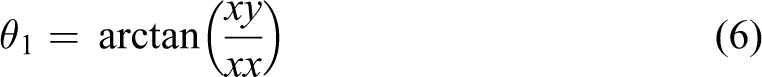
The solution forces the joint angle θ₁ to remain between [−π : π] and joint angle θ₂ to remain between [0 : π]. The joint angular velocity $\dot{θ}$ and acceleration $\ddot{θ}$ are found by differentiating the joint position and velocity.

Feedforward controller

Our feedforward controller is based on the cerebellar model proposed by Kawato. A neural network composes the predictive term while a PD feedback control law is used for stability and for training as shown in Figure 2. As the network adapts to its environment and the arm dynamics, the dependence on the feedback terms reduces.

Figure 2.

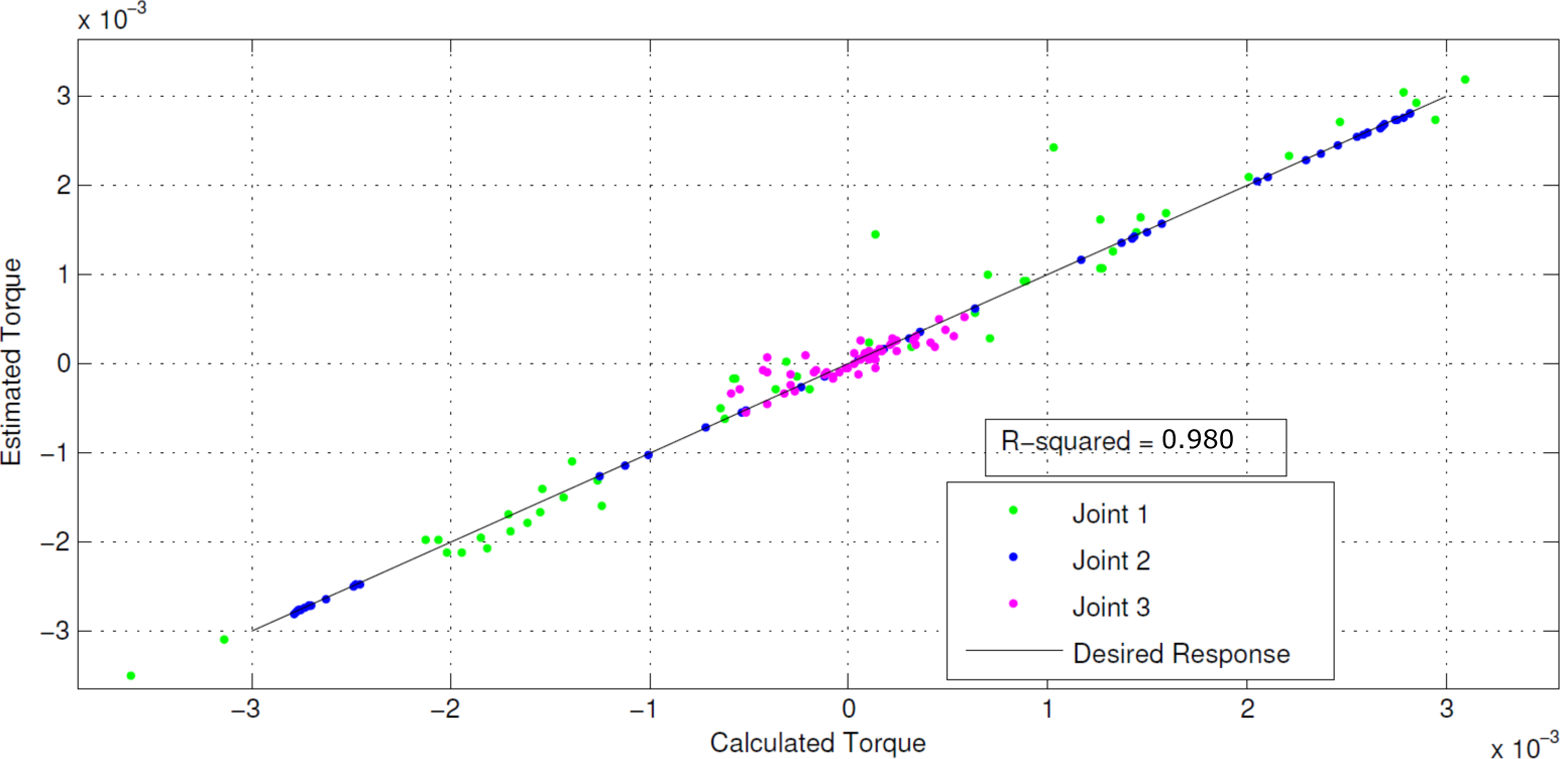
Linear regression of the neural network taught by batch backpropagation.

Neural networks make suitable predictive controllers as it can adapt to complex systems assuming there are enough neurons present in the network.³⁷ Growing and pruning an multilayer perceptron (MLP) neural network has previously been explored,³⁸ and as such, multiple structures were tested until the addition of more neurons no longer improve the network accuracy. As a rover operates in dynamic environments, the controller must also be able to adapt, and therefore, online learning structures have been proposed, namely a backpropagation with momentum (BPM) training law, which was the law used by other researchers in the applications of Kawato’s model.³⁹ A neural network is defined as

b = w_{2} tan h (w_{1} x + w_{1}^{0}) + w_{2}^{0}

where w₁ is the weights acting from the input layer to the hidden layer, $w_{1}^{0}$ is the biases of the hidden layer, w₂ is the weights acting from the hidden layer to the output layer, and $w_{2}^{0}$ is the bias of the output layer. The input to the network is defined as x.

Backpropagation with momentum

The BPM updates the network weights using a gradient method while showing some biasing toward previous training using a momentum vector. The algorithm begins by defining the sum square error E to evaluate the training process

E (x_{k}, w_{k}) = \frac{1}{2} \sum_{n - 1}^{N} \sum_{m - 1}^{M} {(y_{n, k} - b (x_{n, m}, w_{n, m}))}^{2}

where N is the number of training samples (1 for online training), M is the number of network outputs, y_n,k is the desired output, and $b (x_{n, m}, w_{n, m})$ is the current output. The gradient vector g is the first-order derivative of the total error E with respect to the current network weights w_k

g = \frac{\partial E (x_{k}, w_{k})}{\partial w_{k}}

The training law is then defined by the following error gradient

w_{k + 1} = w k - η g + α δ w_{k}

where η is the learning rate and α is the momentum factor.

This structure was found to have problems adjusting to the dynamic environment and so an extended Kalman filter (EKF) training law,^40

–43 which has been showed to work well with online training, was also tested. Neural networks trained online using EKFs have not been used in feedforward control applications.

EKF training algorithm

An EKF combines noisy model and measurements into a weighted estimate of the state. For a neural network, the state is the vector of network weights and the network output is the measurement of the state. The general form of the process equation or the state of an EKF is defined as

w_{k - 1}^{k} = f (w_{k - 1}^{k - 1}, u_{k - 1}) + q_{k}

where $w_{k - 1}^{k}$ is the predicted weights at time k, u_k−1 is the user input to the system, and q_k is the model noise normally distributed about 0 with covariance Q. The function f is the process equation that transforms the weights from time step k − 1 to time step k denoted by $w_{k - 1}^{k}$ . Since the weights of a neural network are not a function of time, nor is it affected by user input, the process equation can be simplified

w_{k - 1}^{k} = w_{k - 1}^{k - 1} + q_{k}

The general form of the EKF measurement equation is defined as

y_{k} = b (w_{k - 1}^{k}) + r_{k}

where y_k is the state measurement at time k and r_k is the measurement noise normally distributed about 0 with covariance R.

The EKF law first predicts the current state $w_{k - 1}^{k}$ and covariance $P_{k - 1}^{k}$

w_{k - 1}^{k} = F_{k - 1}^{k - 1} w_{k - 1}^{k - 1}

P_{k - 1}^{k} = F_{k - 1}^{k - 1} P_{k - 1}^{k - 1} F_{k - 1}^{k - 1, T} + Q

Since the process function is linear, its Jacobian $F_{k - 1}^{k - 1}$ can be found by differentiating the state vector by itself, giving the identity matrix I. The state and covariance prediction simplify to

w_{k - 1}^{k} = w_{k - 1}^{k - 1}

P_{k - 1}^{k} = P_{k - 1}^{k - 1} + Q

The EKF then updates the prediction using the taken measurements. First the Kalman gain is computed

K_{k} = P_{k - 1}^{k} B_{k}^{T} {(B_{k} P_{k - 1}^{k} B_{k}^{T} + R)}^{- 1}

The Jacobian of the neural network B_k, with respect to the weights w, can be broken into four parts

\frac{\partial b}{\partial w_{1}} = w_{2} x (1 - tan h^{2} (w_{1} x + w_{1}^{0}))

\frac{\partial b}{\partial w_{2}} = tan h (w_{1} x + w_{1}^{0})

\frac{\partial b}{\partial w_{1}^{0}} = w_{2} (1 - tan h^{2} (w_{1} x + w_{1}^{0}))

\frac{\partial b}{\partial w_{2}^{0}} = 1

The updated weights $w_{k}^{k}$ and covariance $P_{k}^{k}$ can be determined based on the desired output y_k and current output $b (w_{k - 1}^{k})$ of the neural network

w_{k}^{k} = w_{k - 1}^{k} + K_{k} (y_{k} - b (w_{k - 1}^{k}))

P_{k}^{k} = P_{k - 1}^{k} - K_{k} P_{k - 1}^{k} B_{k}^{T}

Model verification

Feedforward controllers cannot be analyzed using the typical stability techniques. Neural networks performance is quantified using two parameters, the coefficient of determination (R²)⁴⁴ and the mean square error (MSE).⁴⁵ The coefficient of determination indicates how well data points fit a statistical model. In the case of the neural network, the R² value relates how well the output of the neural network maps to the desired output. The R² value is a measure of the accuracy of the neural network. It can be described as

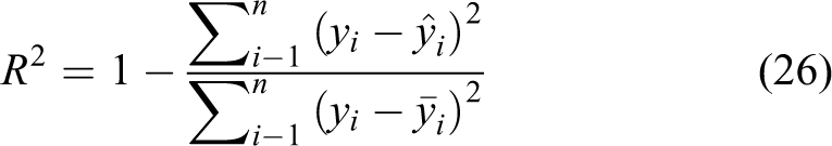
R^{2} = 1 - \frac{\sum_{i - 1}^{n} {(y_{i} - {\hat{y}}_{i})}^{2}}{\sum_{i - 1}^{n} {(y_{i} - {\bar{y}}_{i})}^{2}}

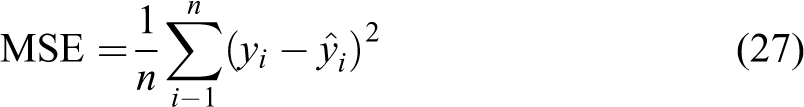
where y_i is the output of the neural network, ${\hat{y}}_{i}$ is the desired response, ${\bar{y}}_{i}$ is the mean value y_i, and n is the number of data points used. The best possible fit has a R² value of 1, and a very poor fit has a R² value of 0.

The other neural network analysis technique is the network MSE. The MSE is a measure of the precision of the network output and describes how close the network output values are to the desired values. It can be described as

MSE= \frac{1}{n} \sum_{i - 1}^{n} {(y_{i} - {\hat{y}}_{i})}^{2}

Simulation results

A simulated version of a 3-DOF pan–tilt unit was constructed in MATLAB. While most pan–tilts are by definition 2-DOF, the hardware used in testing had 3-DOF available, so the decision was made to use a more complex system; the theory being the results should only improve with the reduction in system complexity from 3-DOF to 2-DOF. Feedforward controllers were tested using different network structures and training algorithms to determine whether:

A neural network can adequately predict the dynamics of a 3-DOF pan–tilt camera.

An online training algorithm can be used to adapt a trained network to a dynamic environment.

An online algorithm remains stable while the weights fluctuate during training.

First, to determine whether a neural network could mimic the dynamic equation of a manipulator, a single batch trained network was generated using the Newton–Euler dynamic equations. The output of the trained network versus the desired output is shown in Figure 2.

The network itself had a R² value of 0.980 and an MSE of 5.319 × 10⁻⁸. The near 1 R² and relatively small MSE both indicate a strong correlation between the network and the desired output. They show that the network not only correlates with the statistical data but it is also precise, and it can be concluded that a neural network is capable of mimicking the dynamics of a pan–tilt camera. It should be noted that the fit is not flawless, meaning that the network can never truly be independent of some form of feedback. It can however improve the initial estimation given by the dynamic equations, which will reduce the drift and errors that are being corrected by the feedback signals and allow for greater feedback time delays. Since the batch trained networks are unable to adapt to dynamic environments, an online network was built and tested using the BPM algorithm. The training data set was feed to the network a single point at a time for the entire set. These results are shown in Figure 3.

Figure 3.

Linear regression of the neural network taught by online backpropagation with momentum.

The BPM network had an R² of −0.636 and an MSE of 1.127 × 10⁻⁴. This training algorithm failed to build a usable network. The negative R² means that simply using a mean torque for the entire move would give a better estimate than the neural network. The reason for the poor result is due to the BPM algorithms inability to keep track of past training data, instead biasing the new information over all of the previous training samples. The solution to this problem is to instead use an EKF training algorithm. The EKF algorithm keeps a measure of confidence in the current weights when adding new data points using the covariance matrix. This algorithm was tested using the same method as the BPM algorithm, and the results are shown in Figure 4.

Figure 4.

Linear regression of the neural network taught by extended Kalman filter.

This structure gave an R² value of 0.978 and an MSE of 7.5530 × 10⁻⁷. While this fit is not as good as the batch propagation algorithm, which agrees with other findings, it still was shown to have a high correlation and very low MSE, making it potentially suitable for the pan–tilt application. While after training the network seems to perform well, it’s stability during training is unknown. Stability analysis neural network-based controllers cannot be done using the traditional techniques. In this case, the R² and MSE of the EKF algorithm were monitored during the training process and are shown in Figure 5.

Figure 5.

Training results of the neural network taught by EKF. EKF: extended Kalman filter.

This plot indicates both how fast the algorithm is able to converge to a solution and how to fit changes after each new data sample. In this case, the EKF algorithm was found to converge very quickly, needing fewer than 50 training samples for the R² to remain above 0.95 after beginning with a randomized state. There is also not a lot of variance in R² and MSE during the training, which would suggest some degree of stability over the use of the system. Since the EKF controller was shown to be plausible in simulation, it was then taken and applied in hardware testing on the Barrett WAM.

Barrett WAM results

The EKF controller shown to be a plausible control scheme in the previous section was applied to the Barrett WAM with the goal of determining whether:

An EKF controller can be used to control a pancam allowing it to track objects in the visual field.

An EKF controller can function as well or better than a PD feedback controller.

The Barrett WAM is a 7-DOF manipulator with a spherical wrist. The spherical wrist allows for the decoupling of the displacement and orientation components of the end effector. The decoupling allows for us to easily simulate a full rover/pan–tilt system. The rover itself can be simulated using the displacement of the arm. Moving the first four joints moves the end effector–mounted camera and changes the required viewing orientation. The spherical wrist can simulate the pan–tilt and is able to adjust and control the viewing direction of the camera. In this setup, the arm is told where the target is, and the wrist is tasked with trying to track the object in the visual field using motor commands while the arm itself is being moved. This setup can be seen in Figure 6. While most pan–tilt units in space applications are 2-DOF, it can be assumed if the controller works for a more complex 3-DOF system, it will also work for the simpler 2-DOF model. As with the previous section, in order to compare a feedback controller with a feedforward controller, the R² and MSE values for each were used.

Figure 6.

Configuration of the Barrett WAM.

First a simple PD controller was used to create a control. The controller was tested within the environment described above and the performance is shown in Figure 7. This system had an R² of 0.733 and an MSE of 0.98%. The plot shows a predictable feedback response, where errors need to exist in the system before they can be corrected. Visually, these errors occur as drift where the target moves around a lot in the visual field, occasionally out of the screen.

Figure 7.

Linear regression of feedback control law applied to the Barrett WAM.

The EKF controller was then built and simulated under the same conditions. The linear regression for this controller is shown in Figure 8. The EKF feedforward controller had an R² value of 0.931 and the MSE of 0.18%. The reduction in fit parameters can be attributed to the increase in the complexity of the modeled components. The network is now attempting to predict friction, motor backlash, and so on along with the gravitation, inertial, and Coriolis forces that were used in the MATLAB simulated environment. It is significant to note that the feedforward controller was an improvement over feedback along. Visually, there was less drift and fewer large corrections in the visual field. The tracking was smoother in general; however, it was prone to few jerks when the system came across one of the outlier points.

Figure 8.

Linear regression of EKF trained neural networks applied to the Barrett WAM. EKF: extended Kalman filter.

Conclusions

It was shown that an EKF-trained neural network is able to track objects with a pan–tilt using a 3-DOF spherical manipulator for a model in space rover missions with limited feedback and no images. The EKF network performed better than both a backpropagation model that is normally used and a PD feedback controller.

Feedforward control as shown in this article can also be easily applied to further control applications subject to feedback delays and modeling errors, such as tele-operation of manipulators on the moon or for on-orbit servicing, which is currently considered to be an unsolved problem within robotics.

Footnotes

Declaration of conflicting interests

The author(s) declared no potential conflicts of interest with respect to the research, authorship, and/or publication of this article.

Funding

The author(s) disclosed receipt of the following financial support for the research, authorship, and/or publication of this article: The project was funded by NSERC.

References

Michalski

Bibring

Poulet

. The Mawrth Vallis region of mars: a potential landing site for the Mars Science Laboratory (MSL) mission. Astrobiology 2010; 10: 687–703.

Goldspiel

Squyres

. Ancient aqueous sedimentation on mars. Icarus 1991; 89: 392–410.

Marquez

Fernandez

Anguita

. New evidence for a volcanically, tectonically, and climatically active mars. Icarus 2004; 172: 573–581.

Aloimonos

Weiss

Bandyopadyay

. Active vision. Int J Comput Vision 1988; 1(4): 333–356.

Bajcsy

. Active perception. Proc IEEE 1988; 76: 996–1005.

Marr

. A theory of cerebellar cortex. J Physiol 1969; 202: 437–470.

Albus

. A theory of cerebellar functions. Math Biosci 1971; 10: 25–61.

Albus

. A new approach to manipulator control: the cerebellar model articulation controller (CMAC). J Dyn Syst ASME G 1975; 97: 270–277.

Braitenberg

Atwood

. Morphological observations on the cerebellar cortex. J Compar Neurol 1958; 109: 1–34.

10.

Eccles

Ito

Szentagothai

. The Cerebellum as a neuronal machine. New York: Springer-Verlag, 1967.

11.

Barto

Sutton

Anderson

. Neuronlike adaptive elements that can solve difficult learning control problems. IEEE Trans Syst Man Cyber 1983; 13: 834–841.

12.

Miller

. Real-time application of neural networks for sensor-based control of robots with vision. IEEE Trans Syst Man Cyber 1989; 19: 825–831.

13.

Miller

Kun

. Neural systems for robotics. San Diego: Academic Press, 1997.

14.

Leong

. Kinematics control of redundant manipulators using CMAC neural network. World Multi Syst Cyber Inform 2001; 9: 274–279.

15.

Miall

Weir

Wolpert

. Is the cerebellum a Smith predictor. J Mot Behav 1993; 25: 203–216.

16.

Miall

Wolpert

. The cerebellum as a predictive model of the motor system: a Smith predictor hypothesis. In: Ferrell

Proske

(eds) Neural Control of Movement, New York: Plenum Press, 1995, pp. 215–223.

17.

Paulin

Nelson

Bower

. Neural control of sensory acquisition: the vestibulo-ocular reflex. In: Touretsky

(ed) Advances in Neural Information Processing Systems I, San Mateo: Morgan Kaufmann Publishers, 1989, pp. 410–418.

18.

Paulin

. Evolution of the cerebellum as a neuronal machine for Bayesian state estimation. J Neural Eng 2005; 2: S219–S234.

19.

Paulin

. The role of the cerebellum in motor control and perception. Brain Behav Evol 1993; 41: 39–50.

20.

Paulin

. Neural representations of moving systems. In: Schmahmann

(ed) The Cerebellum and Cognition, San Diego: Academic Press, 1997, pp. 515–533.

21.

Paulin

. A Kalman filter theory of the cerebellum. In: Arbib

Amari

(eds) Dynamic Interactions in Neural Networks: Models and Data, New York: Springer, 1989, pp. 239–259.

22.

Paulin

. A hierarchical neural network model for control and learning of voluntary movement. Biol Cyber 1987; 57: 169–185.

23.

Miller

Sutton

Werbos

. Neural networks for control. Cambridge MA: MIT Press, 1990.

24.

Eckmiller

. Advanced neural computers. Amsterdam: Elsevier Science Publishers, 1990.

25.

Miyamoto

Kawato

Setoyama

. Feedback error-learning neural network for trajectory control of a robotic manipulator. Neural Net 1988; 1: 251–265.

26.

Katayama

Kawato

. Learning trajectory and force control of an artificial muscle arm by parallel-hierarchical neural network model. In: Lippmann

Moody

Touretzky

(eds.) Proceedings of the 1990 conference on Advances in neural information processing systems, Denver Colorado, Vol. 3, 1990, pp. 436–442. San Mateo: Morgan Kaufmann Publishers Inc.

27.

Shibata

Schaal

. Biomimetic gaze stabilization based on feedback-error-learning with nonparametric regression networks. Neural Net 2001; 14: 201–216.

28.

Teshnehlab

Watanabe

. Neural network controller with flexible structure based on feedback-error-learning approach. J Intell Robot Syst 1996; 15: 367–387.

29.

Rao

. Feedback-error learning scheme using recurrent neural networks for nonlinear dynamic systems. IEEE Int Confer Neural Net 1994; 1: 175–180.

30.

Nakanishi

Schaal

. Feedback error learning and nonlinear adaptive control. Neural Net 2004; 17: 1453–1465.

31.

Wolpert

Miall

Kawato

. Internal models of the cerebellum. Trends Cogn Sci 1998; 2: 338–347.

32.

Gilbert

. A real-time video tracking system. IEEE Trans Pattern Anal Mach Intell 1980; PAMI-2: 47–56.

33.

Corke

Goods

. Controller design for high performance visual servoing. World Cong IFAC 1993; 395–398.

34.

Chaumette

Santos

. Tracking a moving object by visual servoing. World Cong IFAC 1993; 9: 409–414.

35.

Kobayashi

Shibata

. Visual tracking of a moving object using a stereo vision robot. Elect Commun Jpn 2008; 91: 19–27.

36.

Park

Hwang

Bahn

. Pan/tilt camera control for vision tracking system based on the robot motion and vision information. IFAC World Cong 2011; 44: 3165–3170.

37.

Antsaklis

. Neural networks for control systems. IEEE Trans Neural Net 1990; 1: 242–244.

38.

Katrayiannis

. Growing radial basis neural networks: merging supervised and unsupervised learning with network growth techniques. IEEE Trans Neural Net 1997; 8: 1492–1506.

39.

Passold

Stemmer

. Feedback error learning neural network applied to a scara robot. In: Kozłowski

(ed.) Proceedings of the fourth international workshop on robot motion and control, Puszczykowo, Poland, 17–20 June 2004, pp. 197–202. New York: IEEE.

40.

Haykin

. Kalman filtering and neural networks. Hoboken: John Wiley & Sons, 2001.

41.

Heskes

Kappen

. On-line learning processes in artificial neural networks. North-Holland Math Library 1993; 51: 199–233.

42.

Singhal

. Training multilayer perceptrons with the extended Kalman algorithm. In: Touretzky

(ed.) Advances in neural information processing systems-I. San Mateo, CA: Morgan Kaufmann, 1989; pp. 133–140.

43.

Ruck

Rogers

Kabrisky

. Comparative analysis of back propagation and the extended Kalman filter for training multilayer perceptrons. IEEE Trans Pattern Anal Mach Intell 1992; 6: 686–691.

44.

El-din

Smith

. A neural network model to predict the waste water inflow incorporating rainfall events. Water Res 2001; 36: 1115–1126.

45.

Ricca

Jami

Alam

. The potential of artificial neural network (ANN) in optimizing media constituents of citric acid production by solid state bioconversion. Int Food Res J 2012; 19: 491–497.

Panoramic camera tracking on planetary rovers using feedforward control

Abstract

Keywords

Introduction

Background

Kinematic model

Feedforward controller

Backpropagation with momentum

EKF training algorithm

Model verification

Simulation results

Barrett WAM results

Conclusions

Footnotes

Declaration of conflicting interests

Funding

References