Sage Journals: Discover world-class research

Abstract

Identification of robotic systems with hysteresis is the main focus of this article. Nonlinear AutoRegressive eXogenous input models are proposed to describe the systems with hysteresis, with no limitation on the nonlinear characteristics. The article introduces an efficient approach to select model terms. This selection process is achieved using an orthogonal forward regression based on the leave-one-out cross-validation. A sampling rate reduction procedure is proposed to be incorporated into the term selection process. Two simulation examples corresponding to two typical hysteresis phenomena and one experimental example are finally presented to illustrate the applicability and effectiveness of the proposed approach.

Keywords

Nonlinear identification NARX model hysteresis prediction error sum of squares term selection

Introduction

Hysteresis, a memory-dependent, multivalued relation between input and output, is often observed in many robotic systems. The system may exhibit a path-dependent pattern, where multiple outputs are associated with increasing or decreasing but the same input and form a loop under cyclic excitation. It exists in many applications, such as actuators and sensors involving smart materials (e.g. piezoelectrics^1,2 and magnetostrictive materials^3,4) which possess the property of hysteresis in the reaction, and some special robotic systems with hysteretic dynamics like aerial vehicles.⁵ The control of these robots is difficult due to the presence of the high nonlinearity. Such nonlinearity turns to be a limitation of open-loop operations in high-precision applications, results in instabilities in closed-loop operation, and degrades the tracking performance even with the use of feedback control in tracking control application.^6,7 It presents challenges in both analysis and controller design of robotic systems with hysteresis. A mathematical model, therefore, is required to predict and control the behavior of the robotic systems containing hysteresis.

Modeling of hysteresis has in recent years attracted increasing attention in various areas of robotics research, such as friction compensation, control of rubber tube actuator, elastic robot joints, and so on. Many researchers have studied this phenomenon, and many mathematical models have been developed to grasp the dynamic features of hysteresis phenomenon.^8

–11 Two of the most popular models are explained in detail in the following sections.

Preisach model

It was originally developed in the 1930s for magnetic hysteresis and is widely used to describe the hysteresis characteristics of smart materials^12
–14 in recent years. It has attracted considerable interest. Preisach model is a weighted superposition of simple independent delayed relays γ_αβ[u] with α, β corresponding to up and down switching values, respectively.¹⁵ This model can be mathematically expressed as

y (t) = \iint_{α \geq β} ρ (α, β) γ_{α β} [u] (t) d α d β

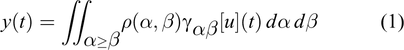
where y(t) and u(t) are the output and input at time t, respectively. ρ(α, β) is known as Preisach density (distribution) function, which weights the single relay units in the α, β - plane and defines the shape of hysteresis curve. The model is regarded as a general description of hysteresis phenomenon with two properties: the casual property and rate-independent property. That is, the output of the model has no relation with future inputs and does not depend on derivatives of the input.

Bouc–Wen model

It was originally proposed by Bouc (1967) and subsequently generalized by Wen (1976). The model has been widely used in the field of structural engineering, which provides reasonable accuracy in the deterministic and stochastic dynamic analyses. The Bouc–Wen model is formulated from mathematical analysis of the characteristic response properties. It is given by the following differential equation

\dot{y} = α \dot{x} - β | \dot{x} | | y |^{μ - 1} y - γ \dot{x} | y |^{μ}

with $α > 0, β + γ > 0, β - γ \geq 0, μ > 1$ . The shapes of hysteresis loops depend on the choice of the loop parameters. In general, α, β, γ influence the loop size, μ the smoothness. The Bouc–Wen model has many advantages. A notable advantage of this model is its capability to capture large numbers of patterns of hysteresis loops with various physical characteristics related to the hysteretic behavior, such as degradation of strength and stiffness,¹⁶ pinching effect,¹⁷ and asymmetry of the peak restoring force.¹⁸ Another advantage of the model is its computational simplicity because only one auxiliary nonlinear differential equation is needed to describe the hysteretic behavior, and the model can be used to analyze the response of the robotic system under any excitation once the parameters have been identified.

Since the nonlinearity of hysteresis may show totally different properties for robotics of different areas, it is impossible to find one accurate model suitable for all types of robotic systems with hysteresis, which not only exists in robot sensors with smart materials but also robot dynamics. The hysteresis can be generally classified into two major categories: static hysteresis and dynamic hysteresis. The former is rate independent, which means there is no correlation between the behavior and the variation rate of input, like the phenomenon corresponding to the Preisach model; while the latter is rate dependent, which depends on the variation rate of input, like the features captured by the Bouc–Wen model.

The purpose of this article is to propose a generalized model with a clear structure in some straightforward way, which can be used to model robotic systems with hysteresis with no limitations on the nonlinear characteristics. The existing models are mostly continuous-time models,^10,12,15 and the mathematical expressions are complicated, such as (1) and (2). One major shortcoming to the use of the continuous-time models is the difficulty of controller design due to the complicated form of the robotic model. Another shortcoming is lack of generalization capability. The nonlinearity and mechanism of hysteresis is different for robotics of different areas. The continuous-time models are given based on parameters with physical meaning, which analyze the mechanism for hysteresis of the particular robot. In addition, continuous-time model is not always available after theoretical analysis of the complex system. Then, discrete-time models can be considered. In practical application, discrete-time observations are obtained and the identification technique is realized by digital computer, so discrete-time models are more convenient in the identification procedure. The authors come up with the idea to use the discrete-time Nonlinear AutoRegressive with eXogenous input (NARX) model to describe the input–output relationship of robotic systems with hysteresis. The NARX model can exhibit a wide range of nonlinear behaviors with different properties such as chaos and bifurcations¹⁹ and can be easily identified. The model structure is constructed in a linear-in-parameter form, which solves the difficulty of controller design.

The article is organized as follows: The NARX model is reviewed in the second section, and analysis for modeling robotic systems with hysteresis is made afterward. The third section introduces the orthogonal forward regression (OFR) algorithm for term selection. The fourth section is devoted to show the limitations of the OFR algorithm, and then an improved model selection procedure with new criteria is developed to solve the problems. Typical simulation examples are discussed in the fifth section, together with the detailed derivations and performance analysis. Experimental example of unmanned aerial vehicle is given in the sixth section. Finally, some concluding remarks are drawn and the limitations of potentially applying the polynomial NARX model to hysteresis identification are discussed in the seventh section. For the sake of easy implementation of digital computers, all the signal processing derived here are based on the discrete-time case.

The NARX model

The NARX representation has attracted considerable interest in modeling nonlinear systems, and many relevant analysis tools and identification algorithms have been developed in recent years.^20

–23 The NARX model is an extension of the linear ARX model. The AR model is used when current output is dependent only on the previous outputs, and the ARX model is used when there is exogenous input given to the AR model, as shown in Figure 1.

Figure 1.

The ARX model.

The NARX model is defined as

y [n] = f (y [n - 1], \dots, y [n - n_{y}], u [n - 1], \dots, u [n - n_{u}]) + e [n]

where y[n] and u[n] are the output and input of the system, respectively; n_y and n_u are the maximum lags for system output and input, respectively; f(⋅) is a nonlinear function which needs to be identified from given observed data; e[n] is the prediction error, which is thought to be a zero mean noise sequence when f(⋅) gives the reasonable description of the nonlinear relation between the output and input. As mentioned in the Introduction, hysteresis is a multivalued and nonsmooth relation between input and output; however, when the input is expanded from u[n] to x [n], where $x [n] = [y [n - 1], \dots, y [n - n_{y}], u [n - 1], \dots, u [n - n_{u}]]$ , corresponding to the definition of NARX model with high-dimensional input spaces, the relationship f(⋅) will turn to be a smooth single-valued mapping, which brings a lot of convenience in the determination of the nonlinear function.

The smooth single-valued function f(⋅) is often constructed by a linear-in-parameter form, using a variety of basic functions $φ_{i} (\cdot)$ , which can be expressed in the regression form

y [n] = \sum_{i = 1}^{n_{m}} θ_{i} φ_{i} (x [n]) + e [n]

where $x [n] = [y [n - 1], \dots, y [n - n_{y}], u [n - 1], \dots, u [n - n_{u}]]$ , $θ_{i} (i = 1, 2, \dots, n_{m})$ are unknown parameters, and n_m is the number of model terms potentially involved. The linear-in-parameter model is widely applied for system identification in many industrial areas, because simple algorithms like least squares method can be used for parameter estimation. If φ_i(⋅) is a polynomial function, the model can be given as²⁴

y [n] = \sum_{m = 0}^{l} \sum_{p = 0}^{m} \sum_{n_{1} = 1}^{n_{y}} \dots \sum_{n_{m} = 0}^{n_{u}} θ_{p, m - p} [n_{1}, \dots, n_{m}] \times \prod_{i = 1}^{p} y [n - n_{i}] \prod_{i = p + 1}^{m} u [n - n_{i}] + e [n]

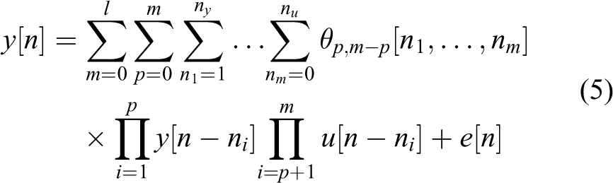
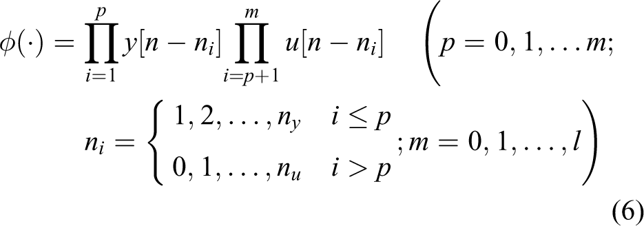
where l is the degree of the polynomial model defined as the maximum order of model terms. Corresponding to (4), φ(⋅) is thus of the form

φ (\cdot) = \prod_{i = 1}^{p} y [n - n_{i}] \prod_{i = p + 1}^{m} u [n - n_{i}] (p = 0, 1, \dots m; n_{i} = {\begin{matrix} 1, 2, \dots, n_{y} & i \leq p \\ 0, 1, \dots, n_{u} & i > p \end{matrix}; m = 0, 1, \dots, l)

Most nonlinear models (e.g. the Volterra series model) only consider the input data to the system as the input to the model. The amount of model terms is sometimes very large; otherwise, the model cannot guarantee the approximation accuracy. The NARX model, however, adds the historical output data to the input variables of the model. The model terms decrease significantly, because the historical output information contains some nonlinear characteristics of the system. So, the NARX model can give a simpler structure for the complex systems. In continuous-time models (1) and (2), integral and differential calculus is needed which adds noise to the identification procedure, as a result algorithm complexity is increased to ensure the accuracy. The NARX model avoids the problem. The discrete-time data can be used directly to approximate the continuous-time system with good performance. The NARX model decomposes the system into a linear segment and a nonlinear segment. The linear segment represents the influence of historical data which deals with problem of rate dependence, while the nonlinear segment (e.g. polynomial form) corresponds to the static nonlinear mapping. The clear structure makes it easier for control design.

OFR algorithm

From (6), it can be easily found out that the total number of terms increases rapidly with the maximum lag $n_{u}, n_{y}$ and degree l. In most application situations, however, only a small percent of the total terms are confirmed to be significant to the performance of the model, so it is necessary to find a method to select model terms. On one hand, redundant terms must be abandoned to avoid overfitting, on the other hand, the model should be as simple as possible, on the basis of containing key model characteristics of the robotic system. Model structure selection turns out to be a key task in the identification process. The main step of the method is to define a criterion for indicating the significance of each term φ(⋅). Several criteria have been proposed in the literature for NARX models.²⁵ One of the most widely used is the error reduction ratio (ERR) based on the OFR algorithm.²⁶ The authors of this article also use it as a reference of the final chosen term detection method. The vector Φ_j is constructed using the result of the jth model term $φ_{j} (\cdot)$ from given data at each time. Then the jth error reduction ratio, ERR _j (also called the squared correlation coefficient), is defined as

{ERR}_{j} = C (Y, Φ_{j}) = \frac{{〈 Y, Φ_{j} 〉}^{2}}{〈 Y, Y 〉 〈 Φ_{j}, Φ_{j} 〉} = \frac{{(Y^{T} Φ_{j})}^{2}}{(Y^{T} Y) (Φ_{j}^{T} Φ_{j})} = \frac{{(\sum_{i = 1}^{N} y_{i} φ_{j}^{i})}^{2}}{\sum_{i = 1}^{N} y_{i}^{2} \sum_{i = 1}^{N} {(φ_{j}^{i})}^{2}}

The ratio provides an effective means to measure the dependency between the output and each term of the model. Then the significant terms can be selected out gradually based on the OFR algorithm. The procedure is described as follows.

Step 1. Select out the term with the largest ERR.

l_{1} = \arg \max_{1 \leq j \leq n_{m}} {C (Y, Φ_{j})}

Then the first significant term can be selected as $w_{1} = φ_{l_{1}}$ .

Step j. Let r _j represent the residual output vector of the model in the jth step. It is given by

r_{m} = r_{m - 1} - \frac{r_{m - 1} w_{m - 1}}{w_{m - 1}^{T} w_{m - 1}} w_{m - 1}

In the first step, r ₀ = Y . Select out the term with the largest ERR in the remaining terms.

l_{j} = \arg \max_{i \neq l_{k} (1 \leq k \leq j - 1)} {C (r_{j}, Φ_{i})}

Then the jth significant term can be selected as $w_{j} = φ_{l_{j}}$ .

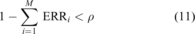
The procedure terminates at the Mth step. M is determined by the terminating condition. For simple situations, it can be given as

1 - \sum_{i = 1}^{M} {ERR}_{i} < ρ

where ERR _i equals $C (r_{i}, Φ_{l_{i}})$ derived in each step, and ρ is the desired error tolerance.

Extension to the OFR algorithm

Limitations of the OFR identification approach

As shown in the third section, the form only considers the tolerance in the identification procedure when all the data are used for fitting. The model usually shows a bad performance when used on future data sets.²⁷ However, in order to be generally used, a model must have good extrapolation properties. It is necessary to split the data into two subsamples: a fitting sample and a validation sample. The fitting sample is used to measure the significance of model terms, while the validation sample is used to terminate the procedure. The fitting sample must contain the key characteristics of the robotic system to ensure that the model identified using the data has the ability to perform the hysteretic behavior with expected properties.

Since the NARX model takes the output history as part of variables in the model, it results in some drawbacks. The model works only when the historical outputs of the robotic system are available. If the output of the robotic system is not measurable in the procedure, the model terms that contain the output need to be calculated by the estimated result of the previous steps, then the system error will be accumulated, leading to inaccuracy in the model.

The data used for identification procedure is obtained from the continuous-time system through periodic sampling

u [n] = u_{c} (n T), y [n] = y_{c} (n T)

where u_c (t), y_c (t) are the continuous-time input and output signals, respectively, and T is the sampling period. T has a tremendous influence on the effectiveness of the final model. The coefficients of the overall model are dependent on the choice of the sampling rate. Practical experience has shown that the mainly influence of sampling rate on modeling is the coefficients of model terms but not the model structure apart from the effects of oversampling.²⁸ Data oversampling will bring numerical problems for nonlinear model structure selection. When the T is chosen to be too small, the fitting data will be so intensive that x [n] ( $x [n] = [y [n - 1], \dots, y [n - n_{y}], u [n - 1], \dots, u [n - n_{u}]]$ ) are highly correlated, which will cause potential problems in distinguishing the significance of model terms. In particular, the output can be extrapolated by the outputs of earlier time as

\begin{array}{l} y [n] = y [n - 1] or \\ y [n] = 2 y [n - 1] - y [n - 2] \end{array}

Then the model finally identified is always a combination of expressions in (13) with a random rule. As a result of that, the model only displays the linearized characteristics at every point, incapable of representing the nonlinear properties of robotic systems with hysteresis. Even if the final model doesn’t end up in the linear form for T_s is small, the ERR of term y[n − 1] is close to 1, while the terms determined by input history, like u[n − 1], u[n − 2], have extremely low ERRs, which will lead to wrong results in the following steps of the OFR procedure after y[n − 1] is selected, since the precision of orthogonalization is influenced profoundly by the noise of data, owing to the strong correlation between model terms. The sampling period, however, cannot be large, in case some important nonlinear information is missed resulting in low approximation accuracy to continuous-time system, especially when rapid change exists in the robotic system.

The PRESS statistic

A commonly used criterion in data splitting is the prediction error sum of squares (PRESS).²⁹ The procedure of leave-one-out cross validation goes like this: remove one observation at a time, use the removed observation as validation point and the remaining N − 1 observations as fitting sample, then estimate the coefficients and evaluate the deleted response ${\hat{y}}_{n}^{(- i)} [i]$ from the estimated model at x = x _i, repeat this process on all points and finally get PRESS residual, defined as

\begin{array}{l} PRESS [n] = \sum_{i = 1}^{N} {[y [i] - {\hat{y}}_{n}^{(- i)} [i]]}^{2} \\ = \sum_{i = 1}^{N} {[ε_{n}^{(- i)} [i]]}^{2} \end{array}

where $ε_{n}^{(- i)} [i]$ is the predicted residual evaluated at the ith point with the fitting sample of size N − 1. Obviously, the computation is complex for the model is to be fitted for N times. Researchers have done much work to simplify the procedure. When using the relationship between the PRESS residual and the ordinal residual, the PRESS reduces to

PRESS [n] = \sum_{i = 1}^{N} {[\frac{ε [i]}{1 - h_{i i}}]}^{2}

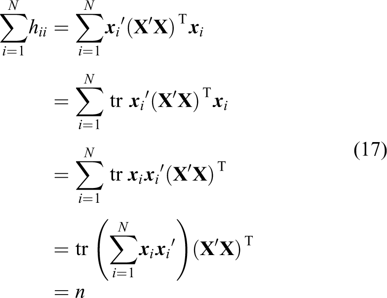
where h_ii represents the prediction variance, given by

h_{i i} = x_{i}' {(X' X)}^{- 1} x_{T}

An important property of h_ii can be easily derived as

\begin{matrix} \sum_{i = 1}^{N} h_{i i} = \sum_{i = 1}^{N} x_{i}' {(X' X)}^{T} x_{i} \\ = \sum_{i = 1}^{N} tr x_{i}' {(X' X)}^{T} x_{i} \\ = \sum_{i = 1}^{N} tr x_{i} x_{i}' {(X' X)}^{T} \\ = tr (\sum_{i = 1}^{N} x_{i} x_{i}') {(X' X)}^{T} \\ = n \end{matrix}

When N >> n,³⁰

PRESS [n] \approx \sum_{i = 1}^{N} \frac{ε^{2} [i]}{(1 - n / N)}

This approximation significantly reduces computational complexity of PRESS.

Considering the problems for model structure selection, a model identified using a finite data set may not have good performance over the fitting data, so the measure of model accuracy has to depend on an additional data set. The cross-validation way helps a lot for the model generalization when substituting the terminating condition of expression (11) with the PRESS statistic in the ORF algorithm. Moreover, the estimated function $\hat{f}$ of (3) provides higher accuracy as the complexity of $\hat{f}$ increases, which is mainly determined by n, the total number of the polynomial NARX model terms. This may cause overfitting to the noise in y[n]. From the simplified expression of PRESS in (18), we can see that the criterion avoids the overfitting phenomenon efficiently because the value of PRESS will increase as n increases owing to the existence of −n in the denominator.

Sampling rate reduction

Following the discussion in “The PRESS statistic” section, the sampling rate must be determined under full consideration of the dynamic characteristics of the data to guarantee that the OFR procedure can capture the main nonlinear effects of the robotic system. When the sampling period is too small, the nonlinear effects will appear to be local linearization, and the OFR procedure will be disturbed by the form of (13). So in situations of very small sampling period, the authors suggest using the improved algorithm followed by sampling rate reduction (SRR) procedure. A decimator in Figure 2, that is, a system with a low-pass filter followed by compression, is required for SRR by integer factor L.

Figure 2.

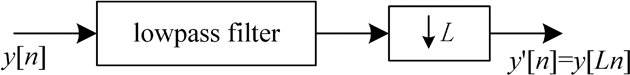
Decimator for sampling rate reduction by L.

The maximum relative deviation (MRD) and the maximum relative error (MRE) are is proposed as the criteria for choice of L in this article. For the new discrete-time data after decimation, with the new sampling period of T′ (=LT), MRD is given as

MRD [T'] = \max_{1 \leq k \leq N / L} {\frac{(y' [k + 2] + y' [k]) / 2 - y' [k + 1]}{y' [k + 1]}}

where y′[k] = y[Lk] is the output of the new discrete-time data. Then the inferior limit of L can be determined by

1 - MRD [T'] < α

where 0 < α < 1 is the expected confidence level. If MRD doesn’t satisfy the inequality, the output y′[n] can be directly derived from the past two points y′[n − 1] and y′[n − 2], that is, the linear relationship in (13) can already reach the requirement of modeling accuracy. The nonlinear information, thus, is not necessary to be contained in the model. However, models which capture little nonlinear characteristics cannot present the nonlinear properties of the robotic system and, certainly, have no significance for controller design in practice.

Then the procedure with SRR is given. First, evaluate the sampling rate 1/T of the original data set D ₀ by the value of MRD. If the value is smaller than 1 − α or very close to it, we may use the following procedure to handle the oversampling data. The data rate is reduced by increasing integer factor L_i (L_i = 2, 3, 4,…) using a decimator, and the value of MRD _i for each new data set D _i with the data rate 1/T_i (T_i = L_iT) is calculated. Note that the MRD _i value is getting bigger as L_i increases, which means local linear regression has less influence on model fitting, whereas some important nonlinear characteristics may be abandoned in the remaining data by the decimator when L_i increases to some extent. So the authors propose the MRE to measure the importance of the information missed due to decimation by L_i , defined as

MRE [L_{i}] = {\begin{array}{l} \max_{1 \leq k \leq N - L_{i}} | \frac{(y [k] + y [k + L_{i}]) / 2 - y [k + L_{i} / 2]}{y [k + L_{i} / 2]} | & L_{i} = 2, 4, 6, \dots \\ \max_{1 \leq k \leq N / L_{i} - 1} {| \frac{(y [k] + y [k + L_{i}]) / 2 - (y [k + (L_{i} + 1) / 2] + y [k + (L_{i} - 1) / 2]) / 2}{(y [k + (L_{i} + 1) / 2] + y [k + (L_{i} - 1) / 2]) / 2} |, & L_{i} = 3, 5, 7, \dots \end{array}

where y[k] is the output of original data set D ₀. The superior limit of decimation factor L is determined by

1 - MRE [L_{i}] > α

where 0 < α < 1 is the expected confidence level. We can choose an appropriate value of L based on the two restrictions in (20) and (22). Then the sampling rate is adjusted to 1/(LT). The model structure is finally selected by the OFR algorithm with the PRESS statistic following this SRR procedure.

Simulation studies

This section investigates the efficiency and performance of the polynomial NARX model for the identification of robotic systems with hysteresis, by applying the OFR algorithm with the PRESS statistic following SRR procedure to two typical examples. The first example is a static hysteresis, given by a simulated Preisach model, while the latter is a dynamic hysteresis, given by a simulated Bouc–Wen model.

A simulated Preisach model

Consider a Preisach model described by the expression as follows

y (t) = \iint_{α \geq β} ρ (α, β) γ_{α β} [u] (t) d α d β + ξ (t)

where $γ_{α β} [u]$ is assumed to be bounded as Figure 3(a), α, β - plane is given as Figure 3(b), ρ(α, β) is assumed to be constant, namely, given as a uniform distribution, and ξ(t) is a Gaussian white noise of zero mean and variance σ² = 0.01. The model is simulated by setting the input signal u(t) as an increasing sequence from −0.5 to 0.5 followed by a decreasing sequence from 0.5 to −0.5 with period 0.01 s, and 202 input–output data point are collected.

Figure 3.

Elements for model in (23): (a) $γ_{α β} [u]$ and (b) α, β - plane.

The model terms φ(⋅) in (4) are chosen to be polynomial functions in (6) determined by the following element: $x [n] = [y [n - 1], y [n - 2], y [n - 3], u [n], u [n - 1], u [n - 2], u [n - 3]]$ , which is the input to the NARX model. First, the SRR procedure is used to adjust the data rate. The values of MRD and MRE in the decimation process are summarized in Table 1.

Table 1.

Evaluation for L in the SRR procedure.

L_i	MRD	MRE	L_i	MRD	MRE
2	0.0129	0.0028	9	0.0425	0.0296
3	0.0155	0.0050	10	0.0480	0.0343
4	0.0192	0.0091	11	0.0534	0.0383
5	0.0233	0.0124	12	0.0589	0.0429
6	0.0276	0.0170	13	0.0631	0.0467
7	0.0324	0.0208	14	0.0711	0.0510
8	0.0372	0.0256	15	0.0745	0.0547

SRR: sampling rate reduction; MRD: maximum relative deviation; MRE: the maximum relative error.

The confidence level is usually expected to be 95% in practice, corresponding to α in expressions (20) and (22), then the decimation factor L can be set to be 11, 12, and 13 according to the results of the SRR procedure. The PRESS values (Table 2), by the OFR algorithm, with different L, over the data set of different size accordingly, are calculated for different model length n.

Table 2.

PRESS values for different model length.

n	PRESS (L = 11)	PRESS (L = 12)	PRESS (L = 13)
6	0.0114	0.0087	0.0062
7	0.0107	0.0085	0.0063
8	0.0106	0.0080	0.0060
9	0.0114	0.0080	0.0059
10	0.0117	0.0088	0.0062
11	0.0126	0.0096	0.0064
12	0.0131	0.0109	0.0081
13	0.0149	0.0137	0.0110

PRESS: prediction error sum of squares.

The PRESS statistic suggests choosing 8 model terms over training data with L = 11 in the SRR procedure, 8 or 9 model terms for L = 12, and 9 model terms for L = 13, and the model terms selected out are almost the same as shown in Table 3.

Table 3.

The term selection results based on the data with different L.

Iter.	Regressors	Parameters (L = 11)	Parameters (L = 12)	Parameters (L = 13)
1	$y^{2} (t - 1)$	0.0631	0.0657	−0.2019
2	u(t)	0.3232	0.3627	0.3871
3	$u (t - 3)$	−0.1703	−0.1924	−0.1921
4	$u^{2} (t)$	−0.3914	−0.0936	−0.1171
5	$u (t) u (t - 3)$	−0.2066	0.1854	0.2293
6	$u^{2} (t - 3)$	–	−0.0967	−0.1056
7	$u^{3} (t)$	0.5929	−0.0513	−0.0758
8	$u^{2} (t - 1)$	0.1577	–	0.0433
9	$y (t - 3)$	0.9664	1.0881	1.1669
Average relative error		0.0015	0.0014	3.3633E−4

The effect of data rate in modeling the robotic systems with hysteresis is sufficiently shown in the results in Table 3. The parameters in the model, but not the model structure, have the strong dependence on the sampling rate. The process also verifies the significance of the SRR procedure and finally shows a good performance for modeling the simulated Preisach model using a polynomial NARX model, which proves that the proposed method is effective for modeling robotic systems with static hysteresis like magnetostrictive actuators.

A simulated Bouc–Wen model

Consider a Bouc–Wen model described in (2), where $α = 1, β = 1, γ = 1, μ = 4.$ The model is simulated by setting the input signal u[n] as a sinusoidal wave and 101 input–output data point are collected. The SRR procedure is not needed, since the sampling rate is low, and the value of MRE doesn’t satisfy the inequality of (22) at L = 2. The leave-one-out cross-validation is carried out directly without the SRR procedure. The input to the model is chosen to be $x [n] = [y [n - 1], y [n - 2], y [n - 3], u [n], u [n - 1], u [n - 2], u [n - 3]]$ , and the polynomial degree is chosen to be l = 3. The result of the PRESS statistic is shown in Figure 4.

Figure 4.

The PRESS statistic versus the model length. PRESS: prediction error sum of squares

It is clear that the model length is best to be 11. The model by choosing 11 model terms is finally identified as

y [n] = 0.3236 y^{3} [n - 1] - 0.4363 u [n - 3] + 0.0183 u^{2} [n - 3] y [n - 3] - 0.2970 u [n - 2] + 0.6885 y [n - 3] - 0.1873 u [n - 1] + 0.1577 u^{2} [n - 2] y [n - 2] + 0.0251 u^{3} [n - 3] + 0.7538 u [n] - 0.1152 u^{2} [n - 1] y [n - 1] - 0.0148 u [n - 1] y^{2} [n - 1]

The model structure identified by the OFR algorithm based on the PRESS statistic is in agreement with traditional modeling assumptions. Figure 5 displays the performance of (24) over the test data set consisting of 120 points. The continuous line is the real values from the simulated Bouc–Wen model, while the dashed line is the estimated output from the NARX model in (24). The relative error of each point is calculated to test the model validity, and the results are given in Figure 6, where the two horizontal lines indicate the desired error tolerance of 5%. The jumping phenomena can be ignored directly, because it is the result of zero values of y[n] in the denominator. Clearly, the model validity tests are well satisfied.

Figure 5.

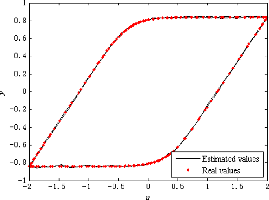
Model performance on the test data.

Figure 6.

Model validity tests for (24).

Experimental result

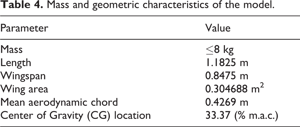
This section aims at illustrating the effectiveness of the NARX model and the accuracy of above explained identification method. For this purpose, we employ an unmanned aerial vehicle for research. The mass and geometric characteristics are shown in Table 4.

Table 4.

Mass and geometric characteristics of the model.

Parameter	Value
Mass	≤8 kg
Length	1.1825 m
Wingspan	0.8475 m
Wing area	0.304688 m²
Mean aerodynamic chord	0.4269 m
Center of Gravity (CG) location	33.37 (% m.a.c.)

In general situations of steady flights with small angle of attack, the models for aerodynamic forces and moments are linear to the state variables. However, for the flights with large angles of attack and sideslip or high angular rates, the forces and moments demonstrate hysteresis effects. The test data of longitudinal large-amplitude sinusoidal motions is investigated. Preisach model cannot apply to this situation, because the hysteresis is relevant to the angular rate. Bouc–Wen model is also inappropriate, because the differential operator on aerodynamic forces and moments will lead to an accumulation of errors. In the study by Greenwell,⁵ a reduced-frequency model is discussed, which was proposed for modeling the hysteresis nonlinearity in aerial vehicle. Comparison of the NARX model and the reduced-frequency model is shown in Figure 7 based on the test data of the normal force coefficient C_N and the angle of attack α with the frequency of 0.4 Hz. The NARX model and the proposed identification approach can be applied to the unmanned aerial vehicle with a high precision.

Figure 7.

Comparison result.

Conclusions

The polynomial NARX model has been considered for modeling robotic systems with hysteresis. The model term selection problem has been investigated for using polynomial NARX models. A critical analysis of the standard OFR algorithm has shown some limitations, particularly when the sampling rate is high. The terminating condition for the OFR algorithm has been modified. The sampling rates over a reasonable range affect the parameter estimates but not affect the model structure. A SRR procedure is proposed based on calculating the MRD and MRE. The applicability and effectiveness of the SRR procedure for term selection have been demonstrated by two simulated examples and one experimental example. Another important property of using polynomial NARX models for hysteresis identification is that few assumption or priori knowledge about the robotic system is needed. When the robotic system is appeared to have a complex noise model, the NARX models should be extended to the nonlinear autoregressive moving average with exogenous variables models.

As a final remark, it should be pointed out that the proposed modeling approach for robotic systems containing hysteresis is not viable for the situation that the previous output data are not available in the process. One solution to this problem is to use the estimated values from the previous steps. However, the solution will cause a stepwise accumulation of errors, owing to the sensitivity of the iteration process to initial condition, so a compensation measure is needed to guarantee the accuracy.

Footnotes

Declaration of conflicting interests

The author(s) declared no potential conflicts of interest with respect to the research, authorship, and/or publication of this article.

Funding

The author(s) disclosed receipt of the following financial support for the research, authorship, and/or publication of this article: This work is supported by the National Natural Science Foundation of China (grant nos 61673240 and 61603210) and the National Program on Key Basic Research Project (grant no 2012613189).

References

Zhang

Tan

. Neural networks based identification and compensation of rate-dependent hysteresis in piezoelectric actuators. Physica B 2010; 405(12): 2687–2693.

Yang

., A modified Prandtl-Ishlinskii model for rate-dependent hysteresis nonlinearity using mth-power velocity damping mechanism. Int J Adv Robot Syst 2014; 11(10): 163.

Shen

. A neural hysteresis model for magnetostrictive sensors and actuators. Int J Adv Robot Syst 2016; 13(4): 1–8.

Chen

Feng

. Adaptive control for continuous-time systems with actuator and sensor hysteresis. Automatica 2016; 64: 196–207.

Greenwell

. A review of unsteady aerodynamic modelling for flight dynamics of manoeuvrable aircraft. In: Atmospheric flight mechanics conference, Providence, Rhode Island, 16–19 August 2004. pp. 1231–1255, 2004, Providence: American Institute of Aeronautics and Astronautics Inc.

Crawley

Anderson

. Detailed models of piezoceramic actuation of beams. J Intell Mater Syst Struct 1990; 1(1): 4–25.

Liu

. Robust adaptive inverse control of a class of nonlinear systems with Prandtl-Ishlinskii hysteresis model. IEEE Trans Autom Control 2014; 59(8): 2170–2175.

Swevers

Al-Bender

Ganseman

., An integrated friction model structure with improved presliding behavior for accurate friction compensation. IEEE Trans Autom Control 2000; 45(4): 675–686.

Hesselroth

Sarkar

Van Der Smagt

. Neural network control of a pneumatic robot arm. IEEE Trans Syst Man Cybern 1994; 24(1): 28–38.

10.

Ruderman

Hoffmann

Bertram

. Modeling and identification of elastic robot joints with hysteresis and backlash. IEEE Trans Ind Electron 2009; 56(10): 3840–3847.

11.

Palli

Borghesan

Melchiorri

. Modeling, identification, and control of tendon-based actuation systems. IEEE Trans Robot 2012; 28(2): 277–290.

12.

Natale

Velardi

Visone

. Identification and compensation of Preisach hysteresis models for magnetostrictive actuators. Physica B 2001; 306(1): 161–165.

13.

Iyer

Tan

Krishnaprasad

. Approximate inversion of the Preisach hysteresis operator with application to control of smart actuators. IEEE Trans Autom Control 2005; 50(6): 798–810.

14.

Xiao

. Modeling and high dynamic compensating the rate-dependent hysteresis of piezoelectric actuators via a novel modified inverse Preisach model. IEEE Trans Control Syst Technol 2013; 21(5): 1549–1557.

15.

Mayergoyz

. Mathematical models of hysteresis. IEEE Trans Magnet 1986; 22(5): 603–608.

16.

Baber

Wen

. Random vibration of hysteretic degrading systems. J Eng Mech Div 1981; 107(6): 1069–1087.

17.

Talatahari

Kaveh

Rahbari

. Parameter identification of Bouc-Wen model for MR fluid dampers using adaptive charged system search optimization. J Mech Sci Technol 2012; 26(8): 2523–2534.

18.

Song

Der Kiureghian

. Generalized Bouc-Wen model for highly asymmetric hysteresis. J Eng Mech 2006; 132(6): 610–618.

19.

PHA

Nguyen

. Novel adaptive forward neural MIMO NARX model for the identification of industrial 3-DOF robot arm kinematics. Int J Adv Robot Syst 2012; 9(4): 104.

20.

Leva

Piroddi

. NARX-based technique for the modeling of magneto-rheological damping devices. Smart Mater Struct 2002; 11(1): 79.

21.

Billings

Wei

. The wavelet-NARMAX representation: a hybrid model structure combining polynomial models with multiresolution wavelet decompositions. Int J Syst Sci 2005; 36(3): 137–152.

22.

Rahrooh

Shepard

. Identification of nonlinear systems using NARMAX model. Nonlin Anal 2009; 71(12): e1198–e1202.

23.

Billings

. Nonlinear system identification: NARMAX methods in the time, frequency, and spatio-temporal domains. New York: John Wiley & Sons, 2013.

24.

Jones

JCP

Billings

. Recursive algorithm for computing the frequency response of a class of non-linear difference equation models. Int J Control 1989; 50(5): 1925–1940.

25.

Falsone

Piroddi

Prandini

. A randomized algorithm for nonlinear model structure selection. Automatica 2015; 60, 227–238.

26.

Chen

Billings

Luo

. Orthogonal least squares methods and their application to non-linear system identification. Int J Control 1989; 50(5): 1873–1896.

27.

Billings

Wei

. An adaptive orthogonal search algorithm for model subset selection and non-linear system identification. Int J Control 2008; 81(5): 714–724.

28.

Billings

Aguirre

. Effects of the sampling time on the dynamics and identification of nonlinear models. Int J Bifurc Chaos 1995; 5(06): 1541–1556.

29.

Allen

. The relationship between variable selection and data augmentation and a method for prediction. Technometrics 1974; 16(1): 125–127.

30.

Miller

. Subset selection in regression. 2nd ed. London: Chapman and Hall, 2002.

Identification of robotic systems with hysteresis using Nonlinear AutoRegressive eXogenous input models

Abstract

Keywords

Introduction

Preisach model

Bouc–Wen model

The NARX model

OFR algorithm

Extension to the OFR algorithm

Limitations of the OFR identification approach

The PRESS statistic

Sampling rate reduction

Simulation studies

A simulated Preisach model

A simulated Bouc–Wen model

Experimental result

Conclusions

Footnotes

Declaration of conflicting interests

Funding

References