Introducing MultiScale technique with CACM-RL

Abstract

Control Adjoining Cell Mapping and Reinforcement Learning (CACM-RL) is a promising technique used to implement controllers. However, it needs many resources so that it can be only applied to simple problems. The contribution of this work is to describe MultiScale approach in order to be used together with CACM-RL technique to overcome its limitations. The main challenge is to verify and validate its efficiency in real-time and in resource-limited systems. MultiScale approach is truly useful when different levels of resolution are needed in the state space, regardless of the number of dimensions. In this way, a set of different regions inside the state space where each region has a specific optimal policy (also different resolutions) is defined. The results described in this article show the feasibility to run MultiScale in real time and find the minimum number of policies to solve the optimal control problem in an automatic way. In the considered test cases, a significant reduction in the total number of cells used is achieved when using MultiScale.

Introduction

Cell-to-cell mapping methods are based on the discretization of the state variables of a system dividing the state space into cells. ¹ A cell-to-cell mapping can be derived from the dynamic evolution of a system. This is of paramount importance, up to the point that if we know the comprehensive cell-to-cell mapping of a system, the system is perfectly characterized. In this sense, there are approaches to design controllers based on cell mapping techniques, such as the simple cell mapping (SCM), ² which carries out the discretization of both state space and control variables and uses a cost function to specify the desired optimality criterion. SCM includes, on the one hand, the efficient application of the numerical methods in order to integrate non-linear systems and, on the other hand, the principle of optimality power in order to search the optimal control efficiently. ² The result is an optimal control method based on a cell state space able to design efficiently the optimal controllers of non-linear systems.

Let Ω be a continuous state space composed of a state vector, x = [x ₁…x_N ], where N is the number of state variables that define the system and x_i is a specific state variable. Then, for each state variable, lower and upper boundaries, x_i ^(l) and x_i ^(u), are specified as follows

$x_i{}^{\left(l\right)}\le x_i\le x_i{}^{\left(u\right)},i=1,\dots ,N$

1

The discretization consists of dividing Ω into cells. Each interval $\left[x_i{}^{\left(i\right)},x_i{}^{\left(u\right)}\right]$ is divided into M intervals with a width of h_i . Each cell is denoted by an index j∈{1…N}. The region located out of, at least, one of the intervals is called the sink cell and it represents the non-interest region. Figure 1 shows a bi-dimensional example of the SCM discretization process.

Figure 1.

Discretization using SCM of a two-dimensional state space. SCM: simple cell mapping.

To illustrate how the discretized state space is merged with the control variables (control actions), a controllability map, ^3,4 such as Figure 2 shows, can be generated in order to assign to each state a specific optimal control action to guide the system to a specific goal.

Figure 2.

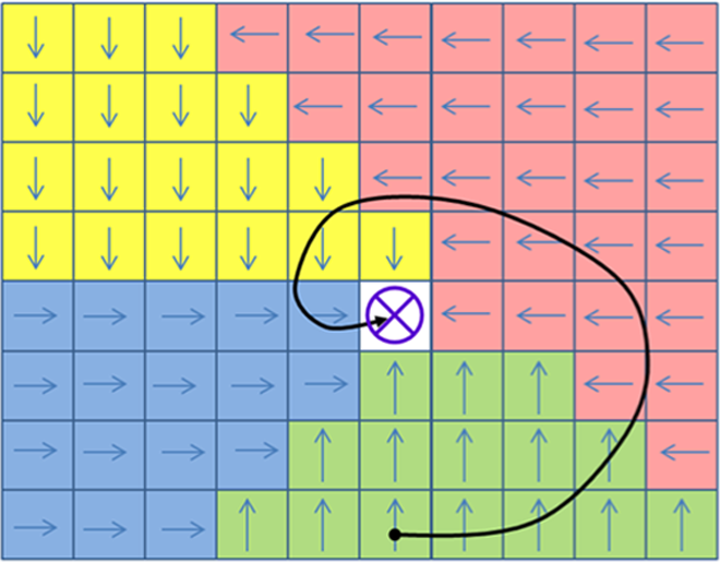
Trajectory that reaches a specific goal. Each type arrow (different colours) refers to the applied control action.

The grid of Figure 2 represents a bi-dimensional system that uses one control vector with four different values (arrows). Applying a specific control action in each state, the system can optimally reach the goal (represented as X).

When working with a high-dimensional state space and with a high number of control actions, and depending on the degree of discretization, there is no doubt that, the needed memory and the use of processor cycles may become a huge problem. Therefore, applying control techniques based on cell mapping requires a great computational effort so that a real-time control on the system is difficult to achieve. The contribution of this work is to propose a feasible algorithm, which is based on cell mapping techniques that allow optimal controllers to work with non-linear and real-time embedded systems. Our contribution with MultiScale represents a unique milestone in the control and planning in real time of dynamic systems using cell mapping techniques because there was not a cell mapping approach to solve optimal control problems in real time so far.

Cell mapping techniques consider the central point of a cell as a reference for the analysis and the cell size as the minimum unit of movement. In this context, it is appropriate to introduce the concept of transition. A transition is the change of system’s state due to a control action applied to the system during a defined period of time. In order to store all possible transitions, it is necessary to make a memory allocation that depends on the number of cells and the number of control actions.

Let Ω denote a k-dimensional state space. In this case, Nc_i is the number of cells for the state variable i, where i = {1, 2,…, k}. Also, let Uc denote a j-dimensional control action vector, where j = {1, 2,…, m}. With these premises, the needed memory records for storing all transitions are, R

$R={\displaystyle \prod _{i=1}^{k}N{c}_i}\cdot {\displaystyle \prod _{j=1}^{m}Uc(j)}$

2

According to equation (2), we have an exponential growth in the number of needed memory records, which makes us to have a constraint in the number of state variables and/or control actions values so that most of the real-time problems (with more than four state variables) may not be solved using cell mapping techniques. Figure 3 shows the memory records required to store all transitions as defined by equation (2). To simplify the graph, we assume that all dimensions have been discretized with the same number of cells.

Figure 3.

Relationship between the state space size (MiB) and the number of cells per state variable considering different number of state variables (dimensions). It is supposed the same number of cells for each variable.

In Figure 3, the dashed lines show the memory required to store the optimal control actions per state. As an illustrative example, 1 GiB memory is required to address the optimal control actions in a five-dimensional state space with 70 cells per dimension. On the one hand, it can be observed that more memory is required if the number of cells per dimension grows. On the other hand, cell size in the discretization process has a direct impact on the accuracy and stability, depending on the dynamics of the system. This means that a compromise solution is required. To alleviate the excessive growing of the state space, a non-uniform discretization can be used. ^5,6 The non-uniform discretization allows improving the processing analysis and, at the same time, obtaining a more accurate and stable control. The main problems associated with the non-uniform discretization are its complexity and the time needed to access the data structures, typically kd-trees. ⁷

In the presented work, a new algorithm named MultiScale is proposed in order to reduce the computational effort and the memory records that store all transitions. It is important to highlight that MultiScale has been designed to be used in real-time control scenarios. Other non-uniform approaches previously described are used in simulated environments, ^5,6 mainly due to the complexity of the search in the state space, which requires a high computational cost.

In our approach, MultiScale is combined with a cell mapping control technique to provide an optimal control solution with a non-uniform discretization. If we compare MultiScale with other cell mapping discretization methods, the needed resources will be dramatically reduced using this new technique. MultiScale is able to select the suitable control policy providing a good balance between resources and requirements. Thanks to this technique, control based on cell mapping methods is feasible in platforms with limited resources, such as embedded systems. With MultiScale, a set of perfectly integrated policies is obtained in a hierarchical structure. MultiScale allows working simultaneously with high resolution when the accuracy is needed and low resolution in other scenarios.

Problems in control based on cell mapping

In this section, we analyse and show a simple case study in order to demonstrate the constraints of control techniques based on cell mapping and applied to dynamic systems in real time. These constraints are mainly related to the cell size (implying a great computational effort and a great use of memory), which cannot be always reduced as much as desired. In addition, the sample period, T_S , could be critical depending on the used specific hardware. The simple study case is referred to the control of the position of a motor. In this example, we analyse in depth optimal control in real time using cell mapping techniques. The goal of the problem is to reach a specific angular position in minimum time. In this case, two state variables have been selected: angular position of the motor, X ₁, and angular velocity, X ₂.

We can see in Figure 4 how several trajectories reach the same goal (origin of coordinates represented by a white dot) from different origin states using a specific control cell mapping technique, called Control Adjoining Cell Mapping and Reinforcement Learning (CACM-RL). ^3,8,9 The way in which the goal is reached is as follows: first, a maximum acceleration is performed and before reaching the goal, an inverse maximum acceleration is applied. In all cases, the goal is reached with a null velocity and no oscillations. The background colour in the graph represents the control action value for each state (on the left side: maximum value; on the right side: minimum value and on the centre cell: no action). The vertical axis is the angular velocity and the horizontal axis is the angular position.

Figure 4.

Controllability map of the DC motor position control problem using a specific control cell mapping technique (CACM-RL). X ₁ (−180°–180°), 41 cells; X ₂ (−1000–1000°/s), 29 cells.

Cell mapping techniques consider the cell size as the minimum unit of movement. The transition time is not constant over all the state space but it is directly related to the dynamics of the system and the cell size. When using control cell mapping techniques, T_s should be always smaller than the transition time. Otherwise, applied control actions could introduce phase delay, and if T_s is greater than the transition time, some undesired oscillations, like those represented in Figure 5, could appear.

Figure 5.

Controllability map of the DC motor position control problem using a specific control cell mapping technique (CACM-RL) and using a T_S greater than the transition time. X ₁ (−180°–180°), 41 cells; X₂ (−1000–1000°/s), 29 cells.

Figure 6 shows a temporal response of the specific controller based on CACM-RL. ^3,8,9 We can see in red, the optimal response when T_s is lower than the transition time. When T_s is higher than the transition time (Figure 5), the response oscillates in a limit cycle. ¹⁰ There is a dependence between cell size, T_S , and the dynamics of the system. Therefore, a suitable cell size should be adjusted according to the dynamics of the system and the computation capabilities. Afterwards, T_S should be chosen.

Figure 6.

Typical temporal response of a DC motor position controller based on CACM-RL.

One of the most relevant characteristics of MultiScale technique presented in this work is its capability to select the most efficient cell size in specific state space areas, always taking into account the lowest T_S , which directly depends on the response time of the system. In this way, computation resources are minimized and optimized. The most practical consequence is the ability to be applied in real time.

MultiScale technique description

The algorithm described in this section, MultiScale, can be used together with any kind of cell mapping technique. In our work, the presented results have been achieved applying MultiScale with the specific technique CACM-RL. ^3,8,9 In this way, we drastically reduce the overall resources in order to compute the control loop in real time. When using CACM-RL, the dk-adjoining constraint ^11,12 is used to adjust automatically the sample period in real time. Thus, we will not have a critical dependence of T_S .

The main difference between MultiScale approach and other previous works ^5,6 is in the method to organize and explore the state space from the continuous world (real): other previous works discretize the continuous control problem into a k-dimensional state space with a variable resolution grid using hypercubes arranged hierarchically in a kd-tree. The root node covers the whole state space. All other nodes are hypercubes covering only a subset of the state space. At every branch, a split is performed in one of the state dimensions, creating two smaller hypercubes. A Kuhn triangulation is implemented at each leaf, effectively splitting it into k! simplexes. The overall effect is a complete triangulation of the space. The value function is interpolated linearly within this triangulation using barycentric coordinates. Figure 7 corresponds to a tree structure where the area covered by each node is indicated in grey level, the splits occur at the centre of every cell (kd-tree) and a Kuhn triangulation is implemented on every leaf level.

Figure 7.

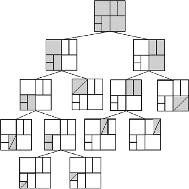
Example of a non-uniform discretization using a kd-tree approach.

MultiScale also discretizes the continuous control problem into a k-dimensional state space but in this case, with a uniform resolution grid per each of the defined regions. The resolution grid of each of the regions depends on the degree of required accuracy. When using a kd-tree approach, the searching complexity is O(n log n), whereas using MultiScale, the complexity is O(1) since the translator functions work on a flat data structure to find a point inside a cell. Figure 8 represents the overall state space with three regions with different resolution grids.

Figure 8.

Example of a non-uniform discretization performed in MultiScale algorithm.

In MultiScale, a uniform discretization in each area of interest is performed. In addition, it can be considered as a non-uniform discretization in an overall view of the state space. However, thanks to the uniform criterion, the translator functions to find a point inside a cell can be applied. If we apply kd-tree in the areas of interest, the most noticeable disadvantage is related to the traceability between the continuous and discrete spaces since it would have to be performed using searches more complex, O(n log n), than using the translator functions, which are O(1). Although we can use kd-tree as a searching method to manage the accuracy in a specific control problem, it would be not as efficient as using MultiScale’s translator functions, and therefore, it would not be feasible to implement in real time.

In general, the high-resolution cell area in a control problem will be given by the degree of accuracy that is required in this area. In order to provide a soft transition among different resolution areas, it is necessary to have an overlap between regions of different resolutions, such as Figure 9 shows. Figure 9 on the left shows a possible trajectory that does not reach the goal. However, in Figure 9 on the right, the trajectory perfectly reaches the goal. Therefore, when working with regions of different resolutions, a frontier with the lowest resolution of the regions must be defined.

Figure 9.

Overlap between regions of different resolutions to ensure a convergence to the goal.

According to Figure 9, the total number of cells per dimension, N_T , can be written in equation form as follows

$N_T=\frac{L}{L_{LR}}+2\cdot \frac{L_{LR}}{L_{HR}}$

3

where L is the total length of the state variable, L_LR is the length of the low-resolution cell and L_HR is the length of the high-resolution cell. Regarding the frontier between two regions of different resolutions, it is necessary to have an overlapping area per each state variable (or dimension). In this case, and in order to see the evolution of the optimality of N_T , we have considered, as a good approximation, half the length of the low-resolution cell (on both sides of the adjoining cell to the goal). In order to achieve the optimal value of N_T , equation (3) is derived with respect to L_LR as follows

${\dot{N}}_T=\frac{-L}{L_{LR}{}^2}+\frac{2}{L_{HR}}$

4

If ${\dot{N}}_T=0$ , the value of L_LR for achieving an optimal value of N_T is

$L_{LR}=\sqrt{\frac{L\cdot L_{HR}}{2}}$

5

Next, Figure 10 shows the variation of N_T for specific values of L_HR . In addition, the optimal variation of N_T is shown using equation (5) in equation (3). In order to illustrate the procedure used in MultiScale, the graphs have been generated for L = 100. In this case, if the final accuracy is specified (L_HR ), we have to select the low resolution (L_LR ) or the total number of cells that we are going to use. One of the two last parameters will give us the other one. Following with the same previous case for L = 100, Table 1 shows a comparison between the total number of cell that should be used for achieving a specific accuracy using a uniform discretization (L_LR = L_HR ) and a non-uniform discretization. Therefore, thanks to MultiScale, state space is reduced more effectively where greater accuracy is required. In this way, we can save computational resources, such as memory, and processor cycles.

Figure 10.

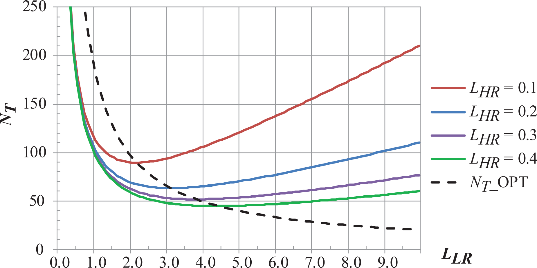
Evolution of N_T with respect to L_LR for different L_HR values and evolution of the optimal variation of N_T function.

Table 1.

Comparison between uniform and non-uniform discretizations.

LHR	LLR	NT (uniform)	NT (non-uniform)	NTU /NTNU
0.1	2.24	1.000	90	11.11
0.2	3.16	500	64	7.82
0.3	3.87	334	52	6.42
0.4	4.47	250	45	5.56

When using MultiScale, the controller has to identify in real time the region where the system is located in order to apply the right control policy. In this case, the particular regionId from the current state is selected using linear functions (lines 1 to 10 in Table 2) and, once inside, the real point must be mapped to the specific cell (regionId2cell in Table 2). It must be taken into account that the regionId can contain in a recursive way other regionId’s with higher resolution. The algorithm shown in Table 2 considers that regionId 0 has the highest resolution and it is embedded in the regionId 1. The latter is embedded in the regionId 2 and so on.

Table 2.

Algorithm used in MultiScale approach to find the control region.

1	$\overrightarrow{\text{x}}\leftarrow \text{current\hspace{0.17em}state}$
2	$\text{SortedRegions}=\text{SortRegionsByResolution\hspace{0.17em}()}$
3	regionId = 0
4	do
5	${\text{x}}_{i\min }=\text{MinimumValue\hspace{0.17em}(SortedRegions}\to \text{regionId,\hspace{0.17em}}{\text{x}}_i)$
6	${\text{x}}_{i\max }=\text{MaximumValue\hspace{0.17em}(SortedRegions}\to \text{regionId,\hspace{0.17em}}{x}_i)$
7	$if(x_i<{\text{x}}_{i\min }\text{\hspace{0.17em}or\hspace{0.17em}}{x}_i>{\text{x}}_{i\max })$
8	$\text{regionId}=\text{regionId}+\text{1}$
9	$\text{i}=\text{i}+\text{1}$
10	$\text{while\hspace{0.17em}(i}<\text{dim(}\overrightarrow{\text{x}}\text{))}$
11	$\text{z}\leftarrow \text{regionId2cell\hspace{0.17em}(regionId,\hspace{0.17em}}\overrightarrow{\text{x}}\text{)}$

The baseline of MultiScale is to consider several regions into the state space with different levels of discretization (see Figure 8) so that the control policies associated with the highest resolution region are embedded in another region with a lower resolution according to the example of Figure 8. The final result is a set of control policies embedded in several areas with different resolutions and therefore different controllability maps, in an overlapped configuration like the one represented in Figure 8.

In order to easily introduce MultiScale technique, we consider that any control problem based on cell mapping techniques can be solved with different policies related to the resolution of the state space. In a general approach, we could use two policies (low resolution and high resolution) to solve the control problem in all state space. This scheme could be recursively applied in order to have several regions (even with different dynamic characteristics) with different resolution levels (policies). Even, it could implement different policies for the same region. Therefore, in this work and with the aim to ease the description of the conceptual ideas of MultiScale technique, we will present MultiScale theory only for two policies taking into account that the explanation can be extended to any number of policies. The high-resolution policy, related to the accuracy requirement, is bounded by the dk-adjoining requirement. ^11,12 This policy is mainly focused on those cases where the motion planning among the states requires accuracy and precision. The low-resolution policy is in charge of solving the motion planning in the rest of the state space where there is no need of accuracy or precision.

When describing MultiScale combined with CACM-RL, it is necessary to take into account one key data structure used in CACM-RL. This data structure is a table called Q-Table(s, a), ⁸ where some of the data stored are accumulated reward for the (s, a)-pair, transition time for the (s, a)-pair and image state that has been transited. From Q-Table(s, a), the optimal policy for each state, a*, is obtained as follows ⁸

$a^{*}\left(s\right)=arg.{\max }_a\left[Q-Table\left(s,a\right)\right]$

6

where s is a specific state and a is the control action associated with s. Q-Table(s, a) is created considering cell sizes defined by the required accuracy and precision; a specific sample period, T_S , which is chosen depending on the response time of the system; and an adjoining distance, dk, which is the key characteristic of CACM-RL and it is an input requirement for the control problem.

In order to define the high-resolution policy, it is required to analyse the control response of the system and to find the boundaries of the region (state space) where dk-adjoining requirement is not met. To do that, we calculate what the maximum dynamics variation of the system per variable, max[ΔXi/Δt], should be in order to have transition distances that meet with the dk-adjoining requirement, and therefore the cell sizes defined initially can be valid.

Due to the fact that Q-Table(s, a) is a bi-dimensional table where the rows are the states of the system in an ordered way and the columns are referred to the different control actions, we can easily identify which states do not meet with the dk-adjoining requirement. The methodology carried out to perform such identification is to take into account two conditions simultaneously: transition time must be higher than T_S and transition distance must meet with the dk-adjoining requirement in all state variables. Therefore, those states whose transitions do not meet with these two conditions should be filtered. When filtering the Q-Table(s, a), a new optimal control table (OCT) is generated, which is only formed by rows or states that meet with the dk-adjoining requirement and by one column that stores the optimal control action associated with each state. In this way, we have generated a high-resolution policy, which is implemented in a bi-dimensional tabular form. The creation of the low-resolution policy is performed considering the rest of states that did not meet with the dk-adjoining requirement in the high-resolution policy. For these states, greater cell sizes are considered in order to meet with the same dk-adjoining condition and for the maximum dynamics variation of the system.

The best way to illustrate the behaviour of MultiScale is to make a comparison with a uniform approach using CACM-RL. ⁸ In Figure 11, we can see two interconnected block diagrams when using CACM-RL. The upper diagram corresponds to the learning process, which uses the received feedback of the system when it interacts with the environment. The lower diagram is referred to the optimal planning process making use of the OCT. Both processes are integrated through the control loop, so it is possible to learn the dynamics and behaviour of the system at the same time as to perform optimal planning.

Figure 11.

Control process using CACM-RL.

Regarding Figure 11, first of all, it is necessary to set a specific goal and the accuracy degree that we have to meet in order to be compliant with the control requirements and dynamics of the system. CACM-RL is implemented according to the study by Gómez et al., ⁸ and it is performed to carry out the following basic functions:

Create the OCT, which is the data structure that stores the optimal control actions associated with each state. CACM-RL searches for the following optimal action in each sample period that should be applied to the system. This data structure is continuously being updated in order to learn during the optimal planning.

Create the Datalog, which is a database that is updated by CACM-RL in each sample period with the feedback received from the output of the plant (state vector). This data structure contains the dynamic behaviour of the system in an implicit way so that CACM-RL needs to use it to achieve the optimal control actions and update the OCT.

If we see Figure 12, using MultiScale combined with CACM-RL, the learning and planning processes consider different resolution grids and specific OCTs for each grid. In general, there could be up to ‘n’ interleaved resolution levels. When using MultiScale, the implementation of CACM-RL is as explained in the study by Gómez et al., ⁸ but in this case, the state space is divided into regions with different resolution levels. Therefore, and due to the fact that we have a non-uniform grid in the state space, the cell() function used in CACM-RL ⁸ (lines 3 and 15 of algorithm 1) should be replaced with the algorithm of Table 2.

Figure 12.

Control process using MultiScale combined with CACM-RL.

Results

To show how MultiScale technique works in real scenarios, two different test cases have been considered: the position control of an electric motor and the optimal motion planning of a vehicle.

Position control of an electric motor

The main goal of this test case is to control the position (angle) of an electric motor by means of the power applied to the motor. This power has been discretized in 15 levels from –100 to +100 power units, so four bits are necessary to identify the control action. In the proposed test, the goal is to reach optimally the final state (X ₁ = 90° and X ₂ = 0°/s) from any initial state. The state space is defined by the angle X ₁ (−180° to 180°) and the angular velocity X ₂ (−1000°/s to 1000°/s). When reaching the goal, the maximum error should be about 1° in position and 1°/s in angular velocity.

The maximum accuracy of the encoder coupled to the motor is 1° and the period for the CACM-RL control loop is 10 ms. We have chosen this period because it is the response time of the motor driver. With the specified requirements, MultiScale evaluates its compliance with d1-adjoining criterion and whether the problem can be solved with a single policy or it is necessary to introduce more policies. The first step is to determine the regions, together with their boundaries, where the single policy complies with the d1-adjoining criterion. If this criterion is met, CACM-RL can provide an optimal controller in all the state space.

In order to find the single policy boundaries, we have to consider the maximum variation of the system per dimension as $\left[\max \left[\frac{\Delta Xi}{\Delta t}\right]Ts \right]$ in 10 ms. Taking into account the cell size (1° in position and 1°/s in velocity) and the d1-adjoining distance, when the system moves with a velocity equal to X ₂ = 1000°/s, it transits 10° (10 units of X ₁ cells) in 10 ms so it would not meet with the d1-adjoining criterion. To avoid the d1-adjoining violation, the maximum range in X ₂ axis is reduced to (−100°/s < X ₂ < 100°/s). According to the previous analysis, the X ₂ boundary in the single resolution policy is defined by ±100°/s. The X ₂ size equal to 1°/s is defined by the accuracy requirements. In the considered example, a second analysis shows that the single policy can also be reduced in X ₁. In this case, the high accuracy is only required in the neighbourhood of the goal, and the performed control far from the goal can be done with a different low-resolution policy. This tuning allows for a significant memory reduction. The advance of X ₁ defines the minimum cell size in the single policy during T_S with the maximum X ₂ real value. Considering X _2max = 826°/s, which is the maximum value tested on the motor, it gives a displacement in X ₁ of 8.26° during T_S = 10 ms. In general, when we need to have a greater accuracy in a high-resolution policy, it is required to increase the dk-adjoining.

When a high accuracy is needed in specific regions of the state space, the best option is to implement MultiScale technique: near the goal or even, in critical trajectories near obstacles. A low-resolution policy will assume the remaining state space with a suitable cell size according to the dynamic range of the system. Table 3 summarizes MultiScale results of the position control of the considered example.

Table 3.

Final cell sizes for high and low resolutions.

	X 1 size	X 2 size	X 1 min	X 1 max	X 2 min	X 2 max
Low-resolution policy	8.26°	200°/s	−180°	180°	−1000°/s	1000°/s
High-resolution policy	1°	1°/s	−9.5°	9.5°	−100.5°/s	100.5°/s

In Tables 4 and 5, the comparison between CACM-RL and CACM-RL combined with MultiScale is shown. It can be seen that CACM-RL requires 722,361 states and MultiScale with only two policies requires 4638 states. These values confirm a great reduction in the use of memory using MultiScale technique.

Table 4.

Final CACM-RL cell sizes and total number of cells.

CACM-RL	Xi size	Cell size	N cells
X 1 space	360°	1°	361
X 2 space	2000°	1°/s	2001
Total cells			722,361

Table 5.

Final MultiScale cell sizes and total number of cells.

MultiScale	Xi size	Cell size	N cells
High resolution
X 1 space	19°	1°	19
X 2 space	201°	1°/s	201
Total cells in high resolution			3819
Low resolution
X 1 space	360°	9.5°	39
X 2 space	2000°	100.5°/s	21
Total cells in low resolution			819
Total cells			4638

Optimal motion planning of a vehicle

The aim of this test case is to plan the motion of a vehicle to reach a specific goal. The origin state is the parked position located at the middle left of Figure 13, and the goal is the parked position located at the bottom right of Figure 13. The vehicle must start from the origin and it shall follow the windy high-speed road until it reaches the goal. The control of the vehicle is optimally performed by CACM-RL in minimum time and taking into account that it should not go off the road. Initially, the vehicle is parked with its front side looking to the left. Therefore, it starts going backwards in order to begin the travel forward. Before reaching the goal, the vehicle must go backwards to park with the same orientation than in origin (front side looking to the left).

Figure 13.

Global vision of the scenario for reaching a goal in minimum time applying MultiScale technique.

MultiScale is used to have specific areas with different resolutions. In this case, parking and curves areas are regions where the accuracy of the motion is more important than in the rest of the road. In Figure 14(a), the optimal trajectory followed by the vehicle has been drawn. We can see how in both curves, the traced path has been planned to reduce the travel time (minimum time criterion). The optimal trajectory does not go by the central axis of the curves. Instead, it goes tangentially to the external or internal zone depending on whether the vehicle enters or leaves the curve. This behaviour occurs because CACM-RL performs a trajectory to reach the goal in minimum time. In this way, the braking is delayed when entering the curve and the acceleration to enter the straight road is applied inside the curve. The controller performs both actions (braking and acceleration) at precise moments to reduce the travel time. This behaviour achieved with CACM-RL is considered an optimal solution. In this sense, it is important to highlight that CACM-RL does not need any input data to generate the trajectory shown in Figure 14(a), but it learns from the experience. ⁸

Figure 14.

(a) Optimal trajectory performed by the vehicle to reach the goal. (b) The sampling of the different vehicle positions along its travel.

In Figure 14(b), different positions of the vehicle along its optimal trajectory (red line) are shown. We can see that it moves at different speeds: using a constant sampling period to acquire its position, the samples (white rectangles) are further apart in the high-speed road than in the parking or curves areas. The yellow rectangles are the occupied parking spaces. Thanks to the implementation of CACM-RL, the vehicle performs a trajectory that avoids these spaces taking into account a security margin.

Figure 15 shows a shade of grey gradients to represent specific control actions in each cell and so we always know the optimal action to be applied to reach the goal in minimum time. Therefore and according to the previous figures, if there are special regions (parking or curves), where we need an accurately planning of the motion of the vehicle or robot, the use of MultiScale technique is the most appropriate approach because it allows us to reduce the computational resources maintaining the optimality.

Figure 15.

Shade of grey gradients that represent specific optimal control actions in each cell.

Conclusions

In this work, a new technique combined with cell mapping algorithms, such as CACM-RL, and named MultiScale has been presented. It has been demonstrated to be a robust and efficient implementation of controllers based on cell mapping since the computation resources are reduced. The most important characteristic of MultiScale is its ability to select the suitable cell size according to the dynamics of the system. In this way, any kind of control problem using cell mapping algorithms can be automatically optimized, ensuring the accuracy and precision required in the design. A simple example with MultiScale applied to the control position of a motor shows a memory resource reduction in the order of 500 times with respect to CACM-RL. This reduction makes possible to apply MultiScale combined with cell mapping algorithm to systems with low resources, such as embedded systems.

Using MultiScale combined with CACM-RL for the resolution of optimal control problems in real time involves a qualitative leap in the technological approaches related to the optimal control of the dynamic systems because there was not a cell mapping approach to solve optimal control problems in real time so far. In this sense and, from the achieved results, the road map of our research group is to apply MultiScale on unstable systems, such as multicopters or an inverted pendulum (light transport vehicle with two wheels) or even on more complex systems with a high number of state variables, such as a fixed-wing aerial platform.