Sage Journals: Discover world-class research

Abstract

For atmospheric entry vehicles, guidance design can be accomplished by solving an optimal issue using optimal control theories. However, traditional design methods generally focus on the nominal performance and do not include considerations of the robustness in the design process. This paper proposes a linear covariance-based model predictive control method for robust entry guidance design. Firstly, linear covariance analysis is employed to directly incorporate the robustness into the guidance design. The closed-loop covariance with the feedback updated control command is initially formulated to provide the expected errors of the nominal state variables in the presence of uncertainties. Then, the closed-loop covariance is innovatively used as a component of the cost function to guarantee the robustness to reduce its sensitivity to uncertainties. After that, the models predictive control is used to solve the optimal problem, and the control commands (bank angles) are calculated. Finally, a series of simulations for different missions have been completed to demonstrate the high performance in precision and the robustness with respect to initial perturbations as well as uncertainties in the entry process. The 3σ confidence region results in the presence of uncertainties which show that the robustness of the guidance has been improved, and the errors of the state variables are decreased by approximately 35%.

Keywords

Entry guidance linear covariance analysis model predictive control robustness

Introduction

Hypersonic entry vehicles may offer a reliable and more cost efficient way to access space by reducing the flight time.¹ Guidance design is challenging since the longitudinal model of the dynamics are known to be unstable and affected by significant model uncertainty.² The entry guidance problem is concerned with providing commands to control the entry vehicles from the initial point to a target point, thus meeting the desired terminal conditions including the position and velocity vector components. During the entry phase, severe constraints on the load limit, dynamic pressure, and heating rate come into action, which must be accounted for and managed well for safety reasons.

Research on entry guidance has been investigated for several decades. The first generation of entry guidance methods was designed for the low-lifting capsule vehicle in the Apollo project.^3,4 In this research, the magnitude and the direction of the spacecraft roll-attitude commands was determined on the in-plane and the roll-attitude ranging requirements respectively. Space shuttle guidance is another milestone in the entry guidance design. In the paper of Harpold and Graves,⁵ they designed a drag acceleration profile by a piecewise analytical function of the velocity which can meet the terminal and path constraints. The results showed that this method is applicable for any entry vehicle with aerodynamic lift which can be used for trajectory control. Subsequently, Mease et al. presented a method to design both the drag and lateral accelerations using a reduced-order model.⁶ Grimm et al. proposed an optimal update scheme for the drag reference profile,⁷ and the guidance was designed in the neighborhood of a specified nominal flight path. Dukeman designed a linear control law using state feedback with energy scheduled gains, which were obtained offline based on a linear quadratic regulator function.⁸ Saraf et al. proposed a guidance method including a trajectory planner and a tracking law.⁹ The planner generated reference drag acceleration and heading angle profiles, while the tracking law commanded the bank angle and the angle of attack to follow the reference profiles.

The drawback of the guidance depending on the reference profile is the lack of robustness. To deal with the disturbances and perturbation, research on the real-time trajectory design and the predictor-corrector entry guidance methods has been carried out in the literature. Shen and Lu presented a method for on board entry trajectory generation.¹⁰ With the quasi-equilibrium glide condition, the problem of meeting the path constraints and designing the longitudinal trajectory profiles were converted into a one-parameter search problem. Lu et al. developed a feedback mechanism for the trajectory control in conjunction with the predictor-corrector guidance method in order to eliminate phugoid oscillations in vehicles with a high lift to drag ratio.¹¹ Xue and Lu proposed a constrained predictor-corrector algorithm that was designed to deal with all common inequality constraints with a modified quasi-equilibrium-glide condition.¹² Brunner and Lu compared the performance of Apollo with that of the numerical predictor-corrector skip entry guidance algorithm and drew the conclusion that high landing precision can be ensured by the numerical predictor-corrector algorithm.¹³ Lu developed an effective predictive load-relief strategy and the simulation showed that the robust longitudinal mode contributes to a satisfactory performance in dispersed cases.¹⁴ In the article by Lu,¹⁵ a single baseline predictor-corrector algorithm has been designed, which was appropriate for vehicles with a wide range of lifting capabilities. Lu also investigated longitudinal lifting entry dynamics and concluded that the flight-path angle dynamics were faster than the altitude by two to three orders of magnitude, which means the time-scale separation is available in gliding entry guidance and trajectory design.¹⁶ In the article by Kamel and Zhang,¹⁷ the authors used the linear model predictive control to solve the problem of trajectory tracking while using the input–output feedback linearization to solve the problem of model nonlinearity.

Real-time trajectory design and predictor-corrector entry guidance methods improve the robustness to some extent. However, this improved robustness is dependent on the redesign of trajectory and guidance commands after the deviation due to disturbances and perturbation. Irrespective of the different improvements made in these methods, a major shortage is that the designed optimality cannot be guaranteed.

Monte Carlo analysis is a common tool used for the robustness analysis of a guidance system. However, Monte Carlo analysis may require several hundreds to thousands of simulation runs which leads to low computation efficiency. Without a mathematical expression, Monte Carlo analysis cannot be used to provide an analytical solution. To overcome these problems, covariance analysis is used to research the effects of environmental and modeling uncertainties on trajectory dispersions instead of Monte Carlo analysis. Zimmer et al. proposed the optimality conditions for a spacecraft to transfer between a set of initial and final conditions using calculus of variations,¹⁸ while minimizing the cost function combined fuel consumption with the estimation error covariance matrix of spacecraft state. Christensen and Geller presented an overview of the covariance analysis for a closed-loop guidance, navigation and control system and demonstrated the capabilities of covariance analysis for the design and analysis of a closed-loop system with guidance, navigation, and a state estimation.¹⁹ Geller developed a new trajectory control and navigation analysis method.²⁰ This method quickly determines trajectory dispersions and navigation errors at specified key points along a reference trajectory. It can be used for the mission design and planning activities, or to determine the best trajectories and the navigation update times to ensure the success of a mission.

This article leverages the advances of linear covariance analysis in the field of trajectory dispersions analysis and explores the use of linear covariance analysis to directly include the trajectory robustness in guidance design. Firstly, in the ‘Entry guidance problem formulation’ section, a dimensionless three degrees of freedom (3 three-degree-of-freedom [DOF]) equation of motion of an entry vehicle is given and all of the entry trajectory constraints are analyzed. Furthermore, in the ‘Linear covariance formulation’ section, the linear covariance analysis is incorporated into the guidance design. A recursive function of a covariance matrix with a feedback updated control input is formulated to provide dispersions along the trajectory, and an innovative cost function is proposed. Subsequently, in the ‘Model predictive control’ section, the model predictive control theory is introduced into the optimal problem solving and the bank angle command under the innovative cost function is calculated. Finally, in the ‘Simulation’ section, simulations with different mission scenarios are run to demonstrate the performance and verify the robustness of the model for state perturbations as well as parametric uncertainties.

Entry guidance problem formulation

Equations of motion

The 3DOF equations of motion of a lifting entry vehicle over a spherical rotating Earth can be expressed as follows¹⁰

\dot{r} = V sin γ

\dot{θ} = \frac{V \cos γ sin ψ}{r \cos ϕ}

\dot{ϕ} = \frac{V \cos γ sin ψ}{r}

\dot{V} = - \frac{D}{m} - g sin γ + ω_{e}^{2} r \cos ϕ (sin γ \cos ϕ - \cos γ sin ϕ sin ψ)

\dot{γ} = \frac{1}{V} [\frac{L \cos σ}{m} + (\frac{V^{2}}{r} - g) \cos γ + 2 ω_{e} V \cos ϕ sin ψ + v ω_{e}^{2} r \cos ϕ (\cos γ \cos ϕ + sin γ \cos ψ sin ϕ)]

\dot{ψ} = \frac{1}{V} [\frac{L sin σ}{m \cos γ} + \frac{V^{2}}{r} \cos γ sin ψ tan ϕ - 2 ω_{e} V (\cos ϕ tan γ \cos ψ - sin ϕ) + \frac{ω_{e}^{2} r}{\cos γ} sin ϕ \cos ϕ sin ψ]

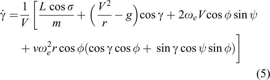
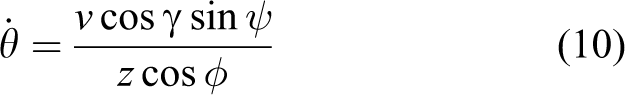
where r is the radial distance from the center of the Earth to vehicle, θ is the longitude, and ϕ is the latitude. In the velocity coordinates, V is the Earth-relative velocity magnitude, γ is the flight-path angle, and ψ is the velocity heading angle which is measured from the north in the clockwise direction. The vehicle mass is m, the gravity is g, and the Earth-rotation rate is ω. L and D are the lift and drag forces expressed as

L = \frac{1}{2} ρ V^{2} S C_{L}

D = \frac{1}{2} ρ V^{2} S C_{D}

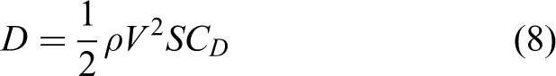
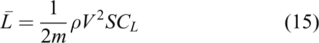
where ρ is the atmospheric density and S is the reference area of the vehicle. $C_{L}$ and $C_{D}$ are aerodynamic lift and drag coefficients as functions of the angle of attack and Mach number.

For the convenience of the analysis and calculations, we use the dimensionless variables

z = \frac{r}{R_{0}}, v = \frac{V}{\sqrt{g_{0} R_{0}}}, τ = \frac{t}{\sqrt{R_{0} / g_{0}}}, Ω = \frac{ω_{e}}{\sqrt{g_{0} / R_{0}}}

to get the dimensionless equations. Where $R_{0}$ is the equatorial radius of the Earth and $g_{0}$ is the gravity at the Earth’s surface.

Then the dimensionless 3DOF equations of motion of a lifting entry vehicle over a spherical rotating Earth are obtained

\dot{z} = sin γ

\dot{θ} = \frac{v \cos γ sin ψ}{z \cos ϕ}

\dot{ϕ} = \frac{v \cos γ sin ψ}{z}

\dot{v} = - \bar{D} - \frac{sin γ}{z} + Ω^{2} z \cos ϕ (sin γ \cos ϕ - \cos γ sin ϕ sin ψ)

\dot{γ} = \frac{1}{v} [\bar{L} \cos σ + \frac{\cos γ}{z} (v^{2} - \frac{1}{z}) + 2 Ω v \cos ϕ sin ψ + Ω^{2} z \cos ϕ (\cos γ \cos ϕ + sin γ \cos ϕ sin ψ)]

\dot{ψ} = \frac{1}{v} [\frac{\bar{L} sin σ}{\cos γ} + \frac{v^{2}}{z} \cos γ sin ψ tan ϕ - 2 Ω v (tan γ \cos ψ \cos ϕ - sin ϕ) + \frac{Ω^{2} z}{\cos γ} sin ϕ \cos ϕ sin ψ]

where the differentiations are with respect to the dimensionless time τ, and the dimensionless lift and drag forces could be respectively expressed as

\bar{L} = \frac{1}{2 m} ρ V^{2} S C_{L}

\bar{D} = \frac{1}{2 m} ρ V^{2} S C_{D}

Entry trajectory constraints

A lifting entry vehicle must obey varies of constraints during its entry process. These include terminal constraints, path constraints, and control constraints. The objective of the guidance design is to find the satisfying state history and the appropriate manipulations of the guidance parameters, namely, the angle of attack and the bank angle within the control bounds to meet the terminal constraints and satisfy the path constraints.

Path constraints

Typical inequality path constraints include the heating rate constraint, the normal load constraint, and the dynamic pressure constraint

\dot{Q} = K {(\frac{ρ}{ρ_{0}})}^{0.5} {(\frac{V}{V_{c}})}^{3} \leq {\dot{Q}}_{max}

n = \frac{L \cos α + D sin α}{m} \leq n_{max}

q = \frac{1}{2} ρ V^{2} \leq q_{max}

where K is a constant related to the vehicle and $V_{c} = \sqrt{g_{0} R_{0}}$ . The right-hand sides of equations (17) to (19) are the specified maximum allowable limits for the heating rate, the normal load, and the dynamic pressure, respectively.

The heating rate is a main constraint in the initial descent due to the high velocity, and then the main constraint becomes the normal load in the mid-velocity phase. In the low-velocity phase, the dynamic pressure is the major constraint to maintain the normal operation of the executive mechanism.

Control constraints

To maintain sufficient controllability, as well as to avoid the stall condition and severe aerodynamic coupling, the angle of attack and the bank angle are constrained by the following relationship

α_{min} (V) \leq α (V) \leq α_{max} (V)

σ_{min} \leq σ \leq σ_{max}

For entry trajectory planning, the angle of attack is usually specified as a function of velocity. In this article, the angle of attack and the bank angle are constrained within $5 ° - 25 °$ and $\pm 75 °$ respectively.

Terminal constraints

The vehicle has to meet the terminal constraints at the final time $τ_{f}$ , and the constraints can be written as

H_{f} = H_{d}, V_{f} = V_{d}, θ_{f} = θ_{d}, ϕ_{f} = ϕ_{d}

where $H_{d}, V_{d}, θ_{d}, and ϕ_{d}$ represent the desired values of the height, velocity, longitude, and latitude, respectively. The variables with subscript f denote the final states obtained through the guidance algorithm.

Linear covariance formulation

Parametric uncertainties

There are several types of uncertainties that affect the entry process which can be modeled in different ways, but the following uncertainties represent what might be encountered and used during the entry guidance process. It is assumed that all uncertainties used in this article are normally distributed with a zero mean and defined standard deviations.

The first type of uncertainty is the initial error. Before the entry process, the vehicle may not arrive at the desired initial point. These errors are in both the initial position states and the velocity states. The values of the errors are given in Table 1.

Table 1.

Initial error parameters.

State	$3 σ$ error	Unit
Altitude	50	km
Longitude	0.05	°
Latitude	0.05	°
Velocity	70	m/s
Flight-path angle	0.2	°
Heading angle	0	°

The second type of uncertainty is in the system dynamics. During the entry process, there are many random disturbances acting on the vehicle due to unmodeled forces. These disturbances are modeled as white Gaussian noise acting on the velocity equations for speed, the flight-path angle, and the heading angle to construct the actual rates

{\dot{v}}_{act} = {\dot{v}}_{n} + η_{v}

{\dot{γ}}_{act} = {\dot{γ}}_{n} + η_{γ}

{\dot{ψ}}_{act} = {\dot{ψ}}_{n} + η_{ψ}

where the subscript n and act mean the nominal and actual stochastic equations of motion respectively. The random variables $η_{v}$ , $η_{γ}$ , and $η_{ψ}$ denote the white noise disturbances.

The initial uncertainties and process noise along the trajectory are easily included in the state deviations along the trajectory by the methods described above. However, the third type of uncertainty is not included in the state directly, but it does impact the state variables. Seywald proposed a method to introduce this type of uncertainty into the covariance calculations.²¹

Including the parameter of interest, $c_{p}$ , the augmented state vector can be given as

x_{a} = [\begin{matrix} x \\ c_{p} \end{matrix}]

The nominal system dynamic becomes

{\dot{x}}_{a} = g_{a} (x, u, c, t) [\begin{matrix} g_{a} (x, u, t) \\ {\dot{c}}_{p} \end{matrix}]

The uncertainty of the parameter is defined as

p_{act} = (1 + c_{p} σ_{p} (x)) p

where $p_{act}$ is the actual parameter considering random processes, $σ_{p}$ is the standard deviation, and p is the value of the nominal parameter. $c_{p}$ is included in the state vector of the system. We can assume that $c_{p}$ is distributed normally with the mean

E [c_{p}] = 0

and variance

E [c_{p}^{2}] = 1

By including $c_{p}$ to the state vector, the third type of uncertainty is modeled within the covariance dynamics, and then it can affect other state errors.

This method is incorporated into the entry guidance design process, allowing the reduction of the sensitivity to different types of uncertainties of the designed trajectory. During the entry process, the uncertainties include aerodynamic coefficients, $C_{L}$ and $C_{D}$ , and the atmospheric density ρ. These uncertainties are characterized as a zero mean, with a $3 σ$ confidence value of $10 %$ of the nominal values. After including the uncertainties as additional states, the augmented state can be written as

x_{a} = [\begin{matrix} x \\ c_{ρ} \\ c_{C_{L}} \\ c_{C_{D}} \end{matrix}]

Covariance dynamics

During the entry process, the precision and optimality of the trajectory is affected by the uncertainties. In order to improve the robustness of the trajectory and reduce the sensitivity to uncertainties, linear covariance analysis theory is introduced into the guidance design process.

Taking the uncertainties into consideration, the system dynamics can be given as

\dot{x} = f (x (t), u (t), t) + g (t) w (t)

where w is the Gaussian white noise of a zero mean, and the covariance is given by

E [w (t) w^{T} (τ)] = R_{w w} (t) δ (t - τ)

where $R_{w w} (t)$ denotes the power spectral density of the white noise.

The covariance of the state variables of a general system can be written as

\begin{matrix} P = E [(x - E [x]) (x - E [x {])}^{T}] \\ = E [(x - x_{N}) (x - x_{N})^{T}] \\ = E (δ x δ x^{T}) \\ = [\begin{matrix} E (δ x_{1} δ x_{1}) & \dots & E (δ x_{1} δ x_{n}) \\ ⋮ & ⋱ & ⋮ \\ E (δ x_{n} δ x_{1}) & \dots & E (δ x_{n} δ x_{n}) \end{matrix}] \end{matrix}

The diagonal components are the variances of each state variable. They represent the deviations of the states from their nominal values. The off-diagonal components describe the correlations between two different state variables.

In order simplify the formulation and use the following theory, the previous system equation (32) is given in discrete form after linearization and discretization

x_{k + 1} = A_{k} x_{k} + B_{k} u_{k} + Γ_{k} w_{k}

where $A_{k} = e^{\frac{\partial f}{\partial x} (k) Δ t}$ , $B = \int_{k}^{k + Δ t} \frac{\partial f}{\partial u} (k) e^{\frac{\partial f}{\partial x} (k) τ} d τ$ , $Γ = \int_{k}^{k + Δ t} \frac{\partial f}{\partial w} (k) e^{\frac{\partial f}{\partial x_{k}} τ} d τ$ .

A nominal reference trajectory can be written as equation (36)

{\hat{x}}_{k + 1} = A_{k} {\hat{x}}_{k} + B_{k} {\hat{u}}_{k}

The dynamics of the linear state covariance with feedback command are given as equation (37)

\begin{matrix} P_{k + 1} = E (δ x_{k + 1} δ x_{k + 1}^{T}) \\ = E {[x_{k + 1} - {\hat{x}}_{k + 1}] [x_{k + 1} - {\hat{x}}_{k + 1}]^{T}} \\ = E {[(A_{k} x_{k} + B_{k} (u_{k} + Δ u_{k}) + Γ_{k} w_{k}) - (A_{k} {\hat{x}}_{k} + B_{k} u_{k})] [(A_{k} x_{k} + B_{k} (u_{k} + Δ u_{k}) + Γ_{k} w_{k}) - (A_{k} {\hat{x}}_{k} + B_{k} u_{k} {)]}^{T}} \\ = E {[A_{k} δ x_{k} + B_{k} Δ u_{k} + Γ_{k} w_{k}] [A_{k} δ x_{k} + B_{k} Δ u_{k} + Γ_{k} w_{k}]^{T}} \\ = A_{k} P_{k} A_{k}^{T} + B_{k} Δ u_{k} Δ u_{k}^{T} B_{k}^{T} + Γ_{k} w_{k} w_{k}^{T} Γ_{k}^{T} \end{matrix}

Equation (37) indicates the relation between the updated control command and the future linear state covariance. In the same way, the final state covariance, $P_{k + 1}$ , is calculated sequentially using a set of future control parameters

\begin{matrix} P_{k + 1} = A_{k} P_{k} A_{k}^{T} + B_{k} Δ u_{k} Δ u_{k}^{T} B_{k}^{T} + Γ_{k} w_{k} w_{k}^{T} Γ_{k}^{T} \\ = A_{k} (A_{k - 1} P_{k - 1} A_{k - 1}^{T} + B_{k - 1} Δ u_{k - 1} Δ u_{k - 1}^{T} B_{k - 1}^{T} \\ + Γ_{k - 1} w_{k - 1} w_{k - 1}^{T} Γ_{k - 1}^{T}) A_{k}^{T} + B_{k} Δ u_{k} Δ u_{k}^{T} B_{k}^{T} \\ + Γ_{k} w_{k} w_{k}^{T} Γ_{k}^{T} \\ = A_{k} A_{k - 1} P_{k - 1} A_{k - 1}^{T} A_{k}^{T} + A_{k} B_{k - 1} Δ u_{k - 1} Δ u_{k - 1}^{T} B_{k - 1}^{T} A_{k}^{T} \\ + B_{k} Δ u_{k} Δ u_{k}^{T} B_{k}^{T} + A_{k} Γ_{k - 1} w_{k - 1} w_{k - 1}^{T} Γ_{k - 1}^{T} A_{k}^{T} \\ + Γ_{k} w_{k} w_{k}^{T} Γ_{k}^{T} \\ = A_{k} A_{k - 1} (A_{k - 2} P_{k - 2} A_{k - 2}^{T} + B_{k - 2} Δ u_{k - 2} Δ u_{k - 2}^{T} B_{k - 2}^{T} \\ + Γ_{k - 2} w_{k - 2} w_{k - 2}^{T} Γ_{k - 2}^{T}) A_{k - 1}^{T} A_{k}^{T} \\ + A_{k} B_{k - 1} Δ u_{k - 1} Δ u_{k - 1}^{T} B_{k - 1}^{T} A_{k}^{T} + B_{k} Δ u_{k} Δ u_{k}^{T} B_{k}^{T} \\ + A_{k} Γ_{k - 1} w_{k - 1} w_{k - 1}^{T} Γ_{k - 1}^{T} A_{k}^{T} + Γ_{k} w_{k} w_{k}^{T} Γ_{k}^{T} \\ ⋮ \\ = K_{1} + K_{2}^{T} Δ U^{T} Δ U K_{2} + K_{3} Q^{T} K_{3}^{T} \end{matrix}

where

\begin{array}{l} K_{1} = \prod_{i = 0}^{k} A_{k - i} \cdot P_{0} \cdot \prod_{i = 0}^{k} A_{i}^{T} \\ K_{2} = [\prod_{i = 1}^{k} A_{k + 1 - i} \cdot B_{0} \prod_{i = 1}^{k - 1} A_{k + 1 - i} \cdot B_{1} \dots A_{k} B_{k - 1} B_{k}]^{T} \\ K_{3} = [\prod_{i = 1}^{j} A_{j + 1 - i} \cdot Γ_{0} \prod_{i = 1}^{j - 1} A_{j + 1 - i} \cdot Γ_{1} \dots A_{j} Γ_{j - 1} Γ_{j}]^{T} \\ Δ U = {[Δ u_{1} Δ u_{2} \dots Δ u_{n - 1}]}^{T} \end{array}

And the initial covariance of the states is given as

P_{0} = E [δ x_{0} δ x_{0}^{T}] = E [(x - x_{0}) (x - x_{0})^{T}]

where $δ x_{0}$ indicates the initial dispersion. x is the real initial state with uncertainties in the form of white noise. $x_{0}$ is the expected initial state.

It is now possible, given a nominal reference trajectory, an initial uncertainty estimate, and a process noise model, to determine the expected state errors at any point by propagating equation (38) along the trajectory.

Model predictive control

Formulation of the control movements

The systems dynamics are considered in their discrete form, the state and output dynamics, which are given by

\begin{array}{l} x_{k + 1} = A_{k} x_{k} + B_{k} u_{k} \\ y_{k} = C_{k} x_{k} \end{array}

where the subscript k means the time epoch. The primary objective is to achieve a suitable control history U, so that the output $y_{n}$ , at the final step n, goes to a desired value of $y_{d}$ . Then the entry guidance problem turns into the optimal control problem. Taking a difference operation on both sides of equation (40), one can obtain

\begin{array}{l} x_{k + 1} - x_{k} = A_{k} (x_{k} - x_{k - 1}) + B_{k} (u_{k} - u_{k - 1}) \\ y_{k} - y_{k - 1} = C_{k} (x_{k} - x_{k - 1}) \end{array}

Let us denote the difference of the state variable and the control variable as $Δ x_{k + 1} = x_{k + 1} - x_{k}$ . With this transformation, the difference of the state-space equations are

\begin{array}{l} Δ x_{k + 1} = A_{k} Δ x_{k} + B_{k} Δ u_{k} \\ Δ y_{k} = C_{k} Δ x_{k} \end{array}

Note that the input to the state-space model is $Δ u_{k}$ . Choosing a new state variable vector ${\bar{x}}_{k} = [Δ x_{k} y_{k}]^{T}$ , we have

\begin{matrix} {\bar{x}}_{k + 1} = [\begin{matrix} Δ x_{k + 1} \\ y_{k + 1} \end{matrix}] = [\begin{matrix} A_{k} & o \\ C_{k + 1} A_{k} & I \end{matrix}] [\begin{matrix} Δ x_{k} \\ y_{k} \end{matrix}] + [\begin{matrix} B_{k} \\ C_{k + 1} B_{k} \end{matrix}] Δ u_{k} \\ y_{k} = [\begin{matrix} o & I \end{matrix}] [\begin{matrix} Δ x_{k} \\ y_{k} \end{matrix}] \end{matrix}

where ${\bar{A}}_{k} = [\begin{matrix} A_{k} & o \\ C_{k + 1} A_{k} & I \end{matrix}]$ , ${\bar{B}}_{k} = [\begin{matrix} B_{k} \\ C_{k + 1} B_{k} \end{matrix}]$ , ${\bar{C}}_{k + 1} = [\begin{matrix} o & I \end{matrix}]$ .

Based on the augmented state-space model, the future state variables are calculated sequentially using a set of future control parameters

\begin{matrix} {\bar{x}}_{1} = {\bar{x}}_{1} \\ {\bar{x}}_{2} = {\bar{A}}_{1} {\bar{x}}_{1} + {\bar{B}}_{1} Δ u_{1} \\ {\bar{x}}_{3} = {\bar{A}}_{2} {\bar{x}}_{2} + {\bar{B}}_{2} Δ u_{2} \\ = {\bar{A}}_{2} ({\bar{A}}_{1} {\bar{x}}_{1} + {\bar{B}}_{1} Δ u_{1}) + {\bar{B}}_{2} Δ u_{2} \\ ⋮ \\ {\bar{x}}_{n} = {\bar{A}}_{n - 1} {\bar{x}}_{n - 1} + {\bar{B}}_{n - 1} Δ u_{n - 1} \\ = {\bar{A}}_{n - 1} ({\bar{A}}_{n - 2} {\bar{x}}_{n - 2} + {\bar{B}}_{n - 2} Δ u_{n - 2}) + {\bar{B}}_{n - 1} Δ u_{n - 1} \\ = ... \\ = \prod_{k = 1}^{n - 1} {\bar{A}}_{n - 1} \cdot {\bar{x}}_{1} + \sum_{k = 1}^{n - 1} (\prod_{i = 1}^{k} {\bar{A}}_{n - 1} \cdot {\bar{B}}_{n - k - 1} Δ u_{n - k - 1}) \end{matrix}

\begin{matrix} y_{n} = {\bar{C}}_{n} {\bar{x}}_{n} \\ = {\bar{C}}_{n - 1} ({\bar{A}}_{n - 2} {\bar{x}}_{n - 2} + {\bar{B}}_{n - 2} Δ u_{n - 2}) \\ ⋮ \\ = {\bar{C}}_{n - 1} \prod_{k = 1}^{n - 1} A_{n - k} \cdot {\bar{x}}_{1} \\ + {\bar{C}}_{e_{N - 1}} \sum_{k = 1}^{n - 1} (\prod_{i = 1}^{k} {\bar{A}}_{n - i} \cdot {\bar{B}}_{n - k - 1} Δ u_{n - k - 1}) \\ = F {\bar{x}}_{1} + G Δ U \end{matrix}

where $F = {\bar{C}}_{n - 1} \prod_{k = 1}^{n - 1} A_{n - k}, G = {\bar{C}}_{n - 1} [\prod_{k = 1}^{n - 2} A_{n - k} \cdot {\bar{B}}_{1} \prod_{k = 1}^{n - 3} A_{n - k} \cdot {\bar{B}}_{2} \dots {\bar{A}}_{n - 1} {\bar{B}}_{n - 2} {\bar{B}}_{n - 1}], Δ U = {[Δ u_{1} Δ u_{2} \dots Δ u_{n - 1}]}^{T}$ .

Note that all of the predicted variables are formulated in terms of the current state variables and the future control movement. The objective is to achieve a suitable set of the errors of the controls to minimize the cost function and the errors in the output.

Cost function selection

Selection of a suitable cost function is one of the key features of any optimal control formulation. One objective in this problem is to minimize the distance of a given location $(θ_{t}, ϕ_{t})$ at the specific terminal height and velocity. In addition, minimization of the deviation of the updated control from its previous value and the total errors of the state variables should be taken into consideration.

The cost function of the following form is considered

J = ε {(y_{n})}^{T} R_{t} ε (y_{n}) + Δ U^{T} R_{c} Δ U + R_{p}^{T} P_{n} R_{p}

where $ε (y_{n}) = [h_{n} - h_{d}, V_{n} - V_{d}, θ_{n} - θ_{d}, ϕ_{n} - ϕ_{d}]^{T}$ , represents a transmission, by which the final state, $y_{n}$ , can be turned into the errors between the predicted final outputs and the desired values, including the height error, velocity error, latitude error, and longitude error. $R_{t}$ , $R_{c}$ , and $R_{p}$ are the weighting matrices, which need to be chosen by the designer.

Bank angle computation

The issue of determining the optimal entry trajectory is to find the required bank angle profile $σ (τ)$ , such that the corresponding trajectory satisfies the initial condition, the terminal constraints, and the path constraints while the cost function can be minimized.

The cost function is expressed as

\begin{matrix} J = ε {(y_{n})}^{T} R_{t} ε (y_{n}) + Δ U^{T} R_{c} Δ U + R_{p}^{T} P_{n} R_{p} \\ = {(F {\bar{z}}_{1} + G Δ U - y_{d})}^{T} R_{t} (F {\bar{x}}_{1} + G Δ U - y_{d}) \\ + Δ U^{T} R_{c} Δ U + R_{p}^{T} (K_{1} + K_{2}^{T} Δ U^{T} Δ U K_{2} \\ + K_{3} Q^{T} K_{3}^{T}) R_{p} \\ = {(F {\bar{x}}_{n - 1} - y_{n})}^{T} R_{t} (F {\bar{x}}_{n - 1} - y_{n}) + K_{1} F {\bar{x}}_{n} - K_{1} y_{n - 1} \\ + R_{p}^{T} (K_{1} + K_{3} Q^{T} K_{3}^{T}) R_{p} + Δ U^{T} G^{T} R_{t} (F {\bar{x}}_{1} - y_{d}) \\ + {(F {\bar{x}}_{1} - y_{d})}^{T} R_{t} G Δ U + Δ U^{T} G^{T} R_{t} G Δ U \\ + Δ U^{T} R_{c} Δ U + R_{p}^{T} K_{2}^{T} Δ U^{T} Δ U K_{2} R_{p} \end{matrix}

The optimality condition calls for the optimal bank angle to satisfy

\frac{\partial J}{\partial Δ U} = 2 (F {\bar{x}}_{1} - y_{d})^{T} R_{t} G + 2 Δ U^{T} G^{T} R_{t} G + 2 Δ U^{T} R_{c} + 2 Δ U^{T} R_{p}^{T} K_{2}^{T} K_{2} R_{p} = 0

Thus, the optimal guidance command can be updated as

Δ U = (y_{d} - F {\bar{x}}_{1}) R_{t} G {(G^{T} R_{t} G + R_{c} + R_{p}^{T} K_{2}^{T} K_{2} R_{p})}^{- 1}

U_{optimal} = U_{initial} + Δ U

We can also use quadratic programming to solve the problem, when the optimal condition cannot be used directly.

Simulation

Vehicle model

The entry vehicle model used in the simulations is the Common Aero Vehicle-H (CAV-H) as shown in Figure 1.

Figure 1.

The CAV-H lifting-body vehicle.

The mass of the vehicle is 907 kg, and the reference area of the vehicle is 0.4839 m². The lift to drag ratios, the coefficients of the lift and drag versus the corresponding angle of attack profile at different Mach numbers are given in Tables 2 to 4.

Table 2.

Lift to drag ratio (L/D).

AOA	Mach 3.5	Mach 5	Mach 8	Mach 10	Mach 15	Mach 20	Mach 23
$10 °$	2.2000	2.5000	3.1000	3.5000	3.3846	3.2692	3.2000
$15 °$	2.5000	2.6616	2.9846	3.2000	3.0846	2.9692	2.9000
$20 °$	2.2000	2.3616	2.6846	2.9000	2.7846	2.6692	2.6000

Table 3.

Coefficient of lift ( $C_{L}$ ).

AOA	Mach 3.5	Mach 5	Mach 8	Mach 10	Mach 15	Mach 20	Mach 23
$10 °$	0.4500	0.4250	0.4000	0.3800	0.3700	0.3600	0.3500
$15 °$	0.7400	0.7000	0.6700	0.6300	0.6000	0.5700	0.5570
$20 °$	1.0500	1.0000	0.9500	0.9000	0.8500	0.8000	0.7800

Table 4.

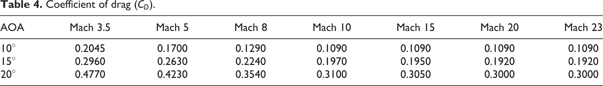
Coefficient of drag ( $C_{D}$ ).

AOA	Mach 3.5	Mach 5	Mach 8	Mach 10	Mach 15	Mach 20	Mach 23
$10 °$	0.2045	0.1700	0.1290	0.1090	0.1090	0.1090	0.1090
$15 °$	0.2960	0.2630	0.2240	0.1970	0.1950	0.1920	0.1920
$20 °$	0.4770	0.4230	0.3540	0.3100	0.3050	0.3000	0.3000

Mission

The limits on the peak heating rate, dynamic pressure, and normal load for all of the missions are listed in Table 5.

Table 5.

Limits of the path constraints.

Path constraints limits	Value
$\dot{Q}$ (kW/m²)	1000
q (kPa)	100
n (g)	4

Simulation with different final conditions

The performance of the proposed linear convariance-based model predictive control (LinCov-MPC) method is verified by simulations of the differen final desired points. The initial nominal conditions and different conditions of the final desired points are listed in Tables 6 and 7.

Table 6.

Initial nominal conditions.

Variables	Value
H (km)	100.00
θ (°)	0.00
ϕ (°)	0.00
V (m/s)	7000.0
γ (°)	−2.0
ψ (°)	45.0

Table 7.

Different final desired conditions at the end of the entry.

Case	$H_{d}$ (km)	$V_{d}$ (m/s)	$θ_{d}$ (°)	$ϕ_{d}$ (°)
1	20.00	2000.0	50.00	50.00
2	20.00	2000.0	50.00	45.00
3	20.00	2000.0	45.00	50.00
4	20.00	2000.0	50.00	40.00
5	20.00	2000.0	40.00	50.00

Five nominal mission scenarios are carried out in the simulations, the trajectory results are shown in Figures 2 to 7 and the corresponding errors of outputs are listed in Table 8.

Figure 2.

Bank angle histories for different cases.

Table 8.

Corresponding errors in the outputs at the end of the entry.

Case	$e_{H}$ (km)	$e_{V}$ (m/s)	$e_{θ}$ (°)	$e_{ϕ}$ (°)
1	0.0042	4.867	−0.0201	−0.0213
2	−0.0082	−5.2345	0.0121	−0.0312
3	0.0106	−2.0413	−0.0371	0.0190
4	0.0073	−3.4223	0.0223	0.0478
5	0.0059	5.9103	0.0309	0.0212

Figure 2 presents the time histories of the bank angle, which are well within the bounds of $\pm 75 °$ . All the bank angles start from zero, fluctuate from 500 s to 1300 s, and become small at the final time. Because of the dispersions in the final desired conditions, each history of the bank angle is slightly different.

The trajectories in the velocity–altitude space are given in Figure 3. The velocity trajectories are decreasing monotonically due to the drag force, while the altitude trajectories decline at first and then climb up a bit when they arrive at the height with a larger atmospheric density which contributes to the considerable lift force. All of the five cases satisfy the terminal constraints in the altitude and velocity at the final points.

Figure 3.

Altitude versus velocity profiles of the entry trajectories for different cases.

Figure 4 shows the latitude trajectories versus the longitude. However, it should be noted that, in each case, the trajectory ends up with $\pm 0.05 °$ error at the final point of entry. The trajectories of all five cases are smooth and satisfy both the terminal longitude and latitude constraints.

Figure 4.

Latitude versus longitude profiles of the entry trajectories for different cases.

The heating rate, normal load and dynamic pressure trajectories for different cases are plotted in Figures 5, 6, and 7 respectively. The heating rate trajectories in Figure 5 illustrate that they keep well within the limit bounds, which is 1000 kW/m² in this article. Figure 6 shows that the normal load variations of the entry trajectories are less than 4 g at all the times in the different cases, satisfying the requirement of the configuration safety. Figure 7 shows that the dynamic pressure trajectories satisfy the path constraints well, and reach a high dynamic pressure at the end of the entry process, which indicates a good control ability.

Figure 5.

Heating rate variations of the entry trajectories for different cases.

Figure 6.

Normal load variations of the entry trajectories for different cases.

Figure 7.

Dynamic pressure variations of the entry trajectories for different cases.

Simulation with perturbations in initial conditions

To adequately test the robustness of the proposed entry guidance method to uncertainties, simulations with perturbations in the initial height, velocity, and flight-path angle are carried out. The different initial conditions are given in Tables 9 and 10.

Table 9.

Different initial conditions.

Case	H (km)	V (m/s)	γ (°)
6	100.00	7000.0	−2.0
7	103.00(+3%)	6986.0(−0.2%)	−1.92(−4%)
8	98.00(−2%)	7028.0(+0.4%)	−2.06(+3%)
9	101.00(+1%)	6944.0(−0.8%)	−1.86(−7%)
10	95.00(−5%)	7021.0(+0.3%)	−1.90(−5%)
11	96.00(+4%)	6973.0(−0.9%)	−2.16(+8%)
12	97.00(−3%)	7042.0(+0.6%)	−2.04(+2%)

Table 10.

Final desired conditions.

Variables	Value
H (km)	20.00
V (m/s)	2000.0
θ (°)	45.00
ϕ (°)	40.00

The trajectory results are plotted in Figures 8 to 12 and the errors in the outputs are listed in Table 11. Figure 8 describes the guidance parameter trajectories of the bank angle σ, which are well within the bounds of $\pm 75 °$ . All the bank angles start from zero, fluctuate from 500 s to 1500 s, and become small at the final time. All trajectories of Cases 7 to 12 are close to the Case 6, which demonstrates the good robustness of the proposed guidance method.

Figure 8.

Bank angle histories for cases with initial perturbations.

Table 11.

Corresponding errors in the outputs at the end of the entry.

Case	$e_{H}$ (km)	$e_{V}$ (m/s)	$e_{θ}$ (°)	$e_{ϕ}$ (°)
6	0.0083	1.0153	−0.0122	−0.0171
7	0.0304	3.1852	−0.0139	−0.0862
8	−0.0102	−6.5985	0.0706	−0.0508
9	0.0106	−1.4138	−0.0861	0.0320
10	0.0211	−4.4902	−0.0675	0.0932
11	0.0394	6.3003	−0.0813	−0.0401
12	−0.0121	3.0011	0.0320	0.0665

The altitude trajectories versus the velocity are plotted in Figure 9. All of the seven cases satisfy the terminal constraints. The velocity trajectories decrease monotonically, while the altitude trajectories decline at first and then climb up a little. All trajectories with different initial perturbations are close to each other, which illustrates the robustness of the proposed guidance method.

Figure 9.

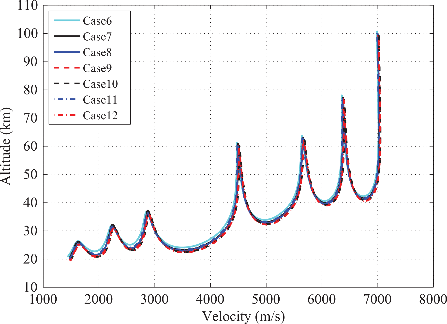
Altitude versus velocity profiles for the cases with initial perturbations.

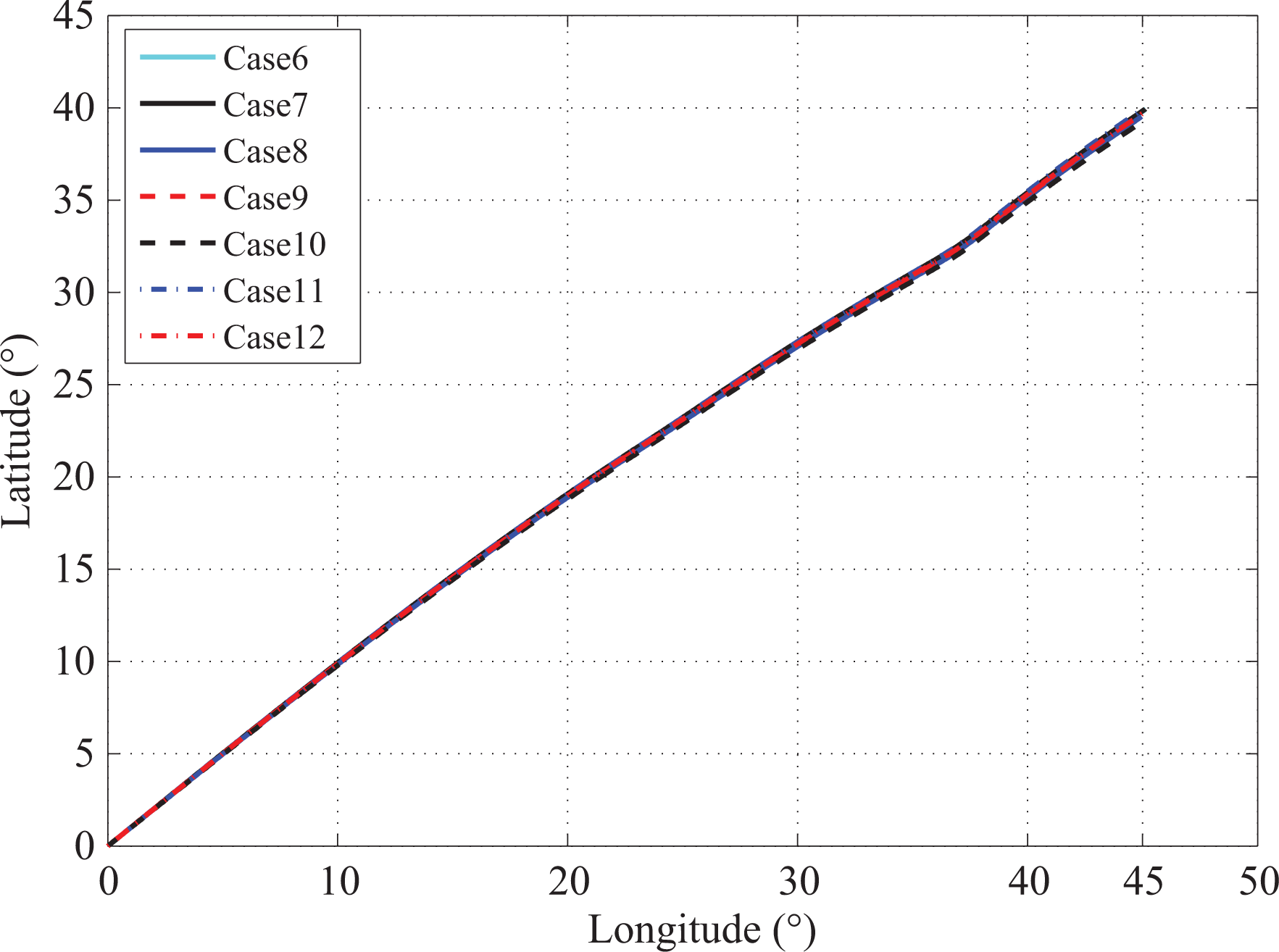
The latitude trajectories versus the longitude are shown in Figure 10. It can be seen that, the trajectories in all of the cases with different initial perturbations ends up with an error of $\pm 0.12 °$ at the final point of the entry. The trajectories of all of the cases are smooth and satisfy the terminal longitude and latitude constraints. The simulations show the robustness of the latitude and longitude trajectories to initial perturbations.

Figure 10.

Latitude versus longitude profiles for the cases with initial perturbations.

The heating rate, normal load, and dynamic pressure of the entry trajectories for different cases are given in Figures 11 to 13. The heating rate trajectories in Figure 11 are well within the allowed bounds. Figure 12 indicates that the normal load of the entry trajectories remains less than 4 g for all of the different cases. Figure 13 illustrates that the dynamic pressure trajectories satisfy the constraints well. And all of the trajectories are close to Case 6, which reveals the robustness of the proposed method.

Figure 11.

Heating rate variations of the cases with initial perturbations.

Figure 12.

Normal load variations of the cases with initial perturbations.

Figure 13.

Dynamic pressure variations of the cases with initial perturbations.

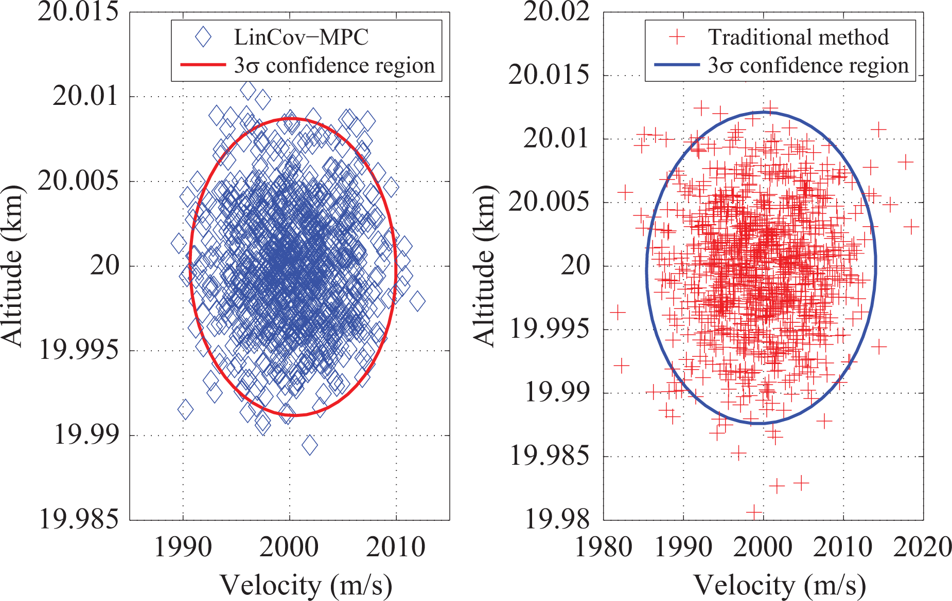
In order to further validate the robustness of the proposed method, 1000 Monte Carlo simulations are carried out for both the traditional method and the proposed method. The initial conditions are based on Table 6 with an additional random distribution within 5% of the height, 1% of the velocity, and 10% of the flight-path angle. The desired final conditions are given in Table 10. The $3 σ$ confidence regions of the state variables errors were found from the simulation results and they sufficiently test the robustness to the perturbation in the initial condition. Figure 14 compares the proposed LinCov-MPC with the traditional method. As expected, the $3 σ$ confidence region of the LinCov-MPC method is smaller than the traditional method. The region is approximately $0.015 °$ smaller in the longitude, and about ${0.02}^{\circ}$ smaller in the latitude. Figure 15 illustrates that the region with $3 σ$ confidence is approximately 3.8 m smaller in altitude, and about 4.1 m/s smaller in velocity.

Figure 14.

Normal load variations of the cases with initial perturbations.

Figure 15.

Dynamic pressure variations of the cases with initial perturbations.

Simulation study with perturbation in the aerodynamic parameters

1000 Monte Carlo simulations have also been conducted to further test the robustness of the proposed guidance method to the perturbation in the atmospheric density and aerodynamic parameters, namely $ρ, C_{L}, and C_{D}$ . The initial nominal conditions and the final desired conditions are listed in Tables 6 and 10. The bounds of the random perturbation are given in Table 12.

Table 12.

Bounds of the random perturbation.

Variables	Bounds
ρ	$\pm 10 %$
$C_{L}$	$\pm 10 %$
$C_{D}$	$\pm 10 %$

Figure 16 shows the results of the longitude and the latitude at the final points in 1000 Monte Carlo simulations. It is clear from this figure that in all of the cases using the proposed method, the errors of the longitude and latitude are within the $0.06 °$ , despite the very large dispersions. In contrast, the $3 σ$ confidence region of the LinCov-MPC method is smaller than the traditional method. The region is approximately $0.021 °$ smaller in the longitude, and about $0.023 °$ smaller in the latitude.

Figure 16.

Longitude and latitude at the final point under perturbations.

The altitude and the velocity at the final points by the different methods in 1000 Monte Carlo simulations are shown in Figure 17. We can note that the errors of the altitude in all of the cases are within 10 m, and the errors of the velocity are within 13 m/s. As expected, the $3 σ$ confidence region of the LinCov-MPC method is smaller than the traditional method. The dispersion region is approximately 6 m smaller in altitude and about 6.3 m/s smaller in velocity.

Figure 17.

Velocity and altitude at the final point under perturbations.

Conclusions

In this article, a LinCov-MPC method for entry guidance design is proposed to improve the robustness to various types of uncertainties. Linear covariance is used to directly introduce guidance robustness, and the errors of the nominal state variables with the feedback guidance commands are innovatively formulated. Then a cost function incorporating covariance is established, and model predictive control theory is used to solve the optimal problem of the guidance design to calculate the bank angle. The new features for the improvement of the robustness developed here prove to be essential to the success of the method in different cases. The simulation results demonstrate the high performance and the robustness with respect to uncertainties. Compared to the traditional method, the proposed one enjoys clear advantages in its robustness. The trajectories with uncertainties are close to the nominal one and the errors of the state variables have decreased by approximately $35 %$ .

Footnotes

Declaration of conflicting interests

The author(s) declared no potential conflicts of interest with respect to the research, authorship, and/or publication of this article.

Funding

The author(s) disclosed receipt of the following financial support for the research, authorship, and/or publication of this article: This work was supported by the Major Program of National Natural Science Foundation of China (grant numbers 61690210 and 61690211).

References

Wang

Sun

. Direct neural discrete control of hypersonic flight vehicle. Nonlinear Dyn 2012; 70(1): 269–278.

Huang

Wang

. Dynamic surface control of constrained hypersonic flight models with parameter estimation and actuator compensation. Asian J Control 2014; 16(1): 162–174.

Moseley

. The Aapollo entry guidance: A review of the mathematical development and its operational characteristics. Task MSC/TRW A-220, TRW Note No. 69-FMT-791 (1969). 1969.

Graves

Harpold

. Apollo experience report: Mission planning for Apollo entry. Report, National Aeronautics and Space Administration, 1972.

Harpold

Graves

CA.

Shuttle entry guidance. In: American Astronautical Society, Anniversary Conference, 25th Houston, TX, 30 October–2 November 1978, vol. 1, p.35.

Mease

Chen

Teufel

. Reduced-order entry trajectory planning for acceleration guidance. J Guid Control Dyn 2002; 25(2): 257–266.

Grimm

van der Meulen

Roenneke

. Update scheme for drag reference profiles in an entry guidance. J Guid Control Dyn 2003; 26(5): 695–701.

Dukeman

. Profile-following entry guidance using linear quadratic regulator theory. AIAA Guidance, Navigation, and Control Conference and Exhibit 2002; 4457: 5–8.

Saraf

Leavitt

Chen

. Design and evaluation of an acceleration guidance algorithm for entry. J Spacecr Rockets 2004; 41(6): 986–996.

10.

Shen

. Onboard generation of three-dimensional constrained entry trajectories. J Guid Control Dyn 2003; 26(1): 111–121.

11.

Forbes

Baldwin

. Gliding guidance of high l/d hypersonic vehicles. In: AIAA Guidance, Navigation, and Control (GNC) Conference, 2013.

12.

Xue

. Constrained predictor-corrector entry guidance. J Guid Control Dyn 2010; 33(4): 1273–1281.

13.

Brunner

. Comparison of fully numerical predictor-corrector and Apollo skip entry guidance algorithms. J Astronaut Sci 2012; 59(3): 517–540.

14.

. Predictor-corrector entry guidance for low-lifting vehicles. J Guid Control Dyn 2008; 31(4): 1067–1075.

15.

. Entry guidance: A unified method. J Guid Control Dyn 2014; 37(3): 713–728.

16.

. Entry guidance using time-scale separation in gliding dynamics. J Spacecr Rockets 2015; 52(4): 1253–1258.

17.

Kamel

Zhang

. Linear model predictive control via feedback linearization for formation control of multiple wheeled mobile robots. In: IEEE international conference on information and automation, 8 August 2015, pp. 1283–1288. IEEE.

18.

Zimmer

Ocampo

Bishop

. Reducing orbit covariance for continuous thrust spacecraft transfers. IEEE Trans Aerosp Electron Syst 2010; 46(2): 771–791.

19.

Christensen

Geller

. Linear covariance techniques for closed-loop guidance navigation and control system design and analysis. Proc Inst Mech Eng G J Aerosp Eng 2012; 228(1): 44–65.

20.