Bidirectional scale-invariant feature transform feature matching algorithms based on priority k -d tree search

Abstract

In this article, a bidirectional feature matching algorithm and two extended algorithms based on the priority k-d tree search are presented for the image registration using scale-invariant feature transform features. When matching precision of image registration is below 50%, the discarding wrong match performance of many robust fitting methods like Random Sample Consensus (RANSAC) is poor. Therefore, improving matching precision is a significant work. Generally, a feature matching algorithm is used once in the image registration system. We propose a bidirectional algorithm that utilizes the priority k-d tree search twice to improve matching precision. There are two key steps in the bidirectional algorithm. According to the case of adopting the ratio restriction of distances in the two key steps, we further propose two extended bidirectional algorithms. Experiments demonstrate that there are some special properties of these three bidirectional algorithms, and the two extended algorithms can achieve higher precisions than previous feature matching algorithms.

Introduction

Image registration is the way of overlaying two or more images of the same scene taken at different times, from different viewpoints. Registration methods mainly include feature detection, feature matching, transform model estimation, and image resampling and transformation. Area-based and feature-based methods are the two main approaches in feature detection. ¹ Lowe proposed a scale-invariant feature transform (SIFT) feature that represents the image gradients within a local region of an image. ² The SIFT feature is invariant to image rotation and scale and robust across many affine transformations. Because of the invariant to image transformations, lots of solutions based on SIFT features have been integrated into realistic applications, such as object recognition ^3,4 and video tracking. ^{5 –7} Cheung and Hamarneh ⁸ presented an n-dimensional SIFT method for extracting and matching salient features from scalar images of arbitrary dimensionality. Recently, SIFT feature–based methods in image registration have been widely studied. An algorithm integrating the intensity variations and SIFT features of ultrasound images was developed in nonrigid registration. ⁹ Brown and Lowe applied SIFT features in their automatic panoramic image stitching system. ¹⁰ The registration step may take advantage of SIFT-based correspondence to estimate the transformation between images. ¹¹ The dimension of SIFT feature recommended by Lowe ² is 128 and very high. Feature matching will largely affect the performance of image registration system based on SIFT features.

The main methods for SIFT feature matching are the linear search, hash tables, and k-d tree search. The linear search has lower speed, and hash tables perform well in low dimensions but poorly in high dimensions. The k-d tree structure was firstly proposed in the research by Schauer and Nuchter ¹² for associative searching. The value of the notation k is the dimension of features which are applied to build a k-d tree. Little time was spent on building a k-d tree, but lots of computation works are needed to find the best matches. The original k-d tree was optimized to minimize the expected number of nodes need to be examined. ¹³ The optimized tree that can significantly reduce the cost of calculation is theoretically a balance tree. The combination of the search algorithm ¹² and the improved method of building the k-d tree ¹³ is called the standard k-d tree search (shortly named “standard search”), which has a theoretical logarithmic search time in low dimensions. But in high dimensions, ¹⁴ its search time increases sharply because of the cost of backtracking through the tree to return the exact nearest neighbor (NN).

Some variations of a k-d tree were proposed to improve the performance in high dimensions. The priority k-d tree search (shortly named “priority search”) was an efficient and approximate NN search algorithm. ^15,16 It modified the search order of the standard search algorithm and searched subtrees in the order of their closest distance from the query feature. A sorted list was required to store the subtrees in order to efficiently determinate the search order. Beis and Lowe developed the Best Bin First (BBF) algorithm, ¹⁷ which is the same as the priority search. The priority technique has been applied in many systems. ^2,18,19

The randomized trees for fast matching were firstly introduced in a study by Amit and Geman ²⁰ and then used in the work done by Lepetit and Fua. ²¹ Silpa-Anan and Hartley ²² used multiple randomized k-d trees which concerned with the more geometric problem of NN search, to speed up searching. But it takes much time to build multiple randomized trees. Muja and Lowe ²³ described a system that selects the better algorithm and optimizes the parameters automatically, and it needs an example of data set and the desired precision.

In an image registration system, there are generally hundreds or thousands of SIFT features of an image, but several of them can be used to align images. The discarding wrong match performance of many robust fitting methods like Random Sample Consensus (RANSAC) is poor, when matching precision of image registration is below 50%. So, improving matching precision is a significant work. In the following of this article, we will state “the matching precision” as “the precision” shortly. In the work done by Brown and Lowe, ¹⁰ the priority search is used only once where SIFT features between two images are matched. The SIFT features of one image are used to build a k-d tree, and a search algorithm runs on this tree to return the NN of each SIFT feature of another image. In order to improve matching precision, in this article, we propose a bidirectional SIFT feature matching (BSFM) algorithm and two extended algorithms based on the priority search. The priority search is used twice in these three bidirectional algorithms. Lowe stated that if the ratio of distance of the closest neighbor to distance of the second closest neighbor for each query feature is not greater than 0.8, the match between the closest neighbor and query feature is accepted, otherwise abandoning it. ² Thus, the features that did not have good match to the query feature set can be discarded. According to the case of adopting the ratio restriction of distances, we present two extended bidirectional algorithms based on the BSFM algorithm.

The remainder of this article is organized as follows. Section “Priority k-d tree search algorithm” is the brief introduction of the priority search. Three different bidirectional algorithms are proposed in section “BSFM algorithms.” In section “Experiments,” we compare the performance of different algorithms, including the linear search, the standard search, the priority search and three proposed bidirectional algorithms. In the final section, the conclusions are presented.

Priority k-d tree search algorithm

Process of building the standard version of the k-d tree

In this section, we take a brief review about the process of building the standard version of the k-d tree. The standard version of the k-d tree search algorithm was first proposed by Friedman et al. ²⁴ The following is a brief review of the k-d tree. First, find out the ith dimension with the greatest variance in the SIFT feature data set. The ith dimension is the discriminating dimension of the root node. The value of the SIFT feature in the ith dimension that is closest to the median value in the ith dimension is the partition value. Then, choose the SIFT feature as the root node. The partition value in the ith dimension is the threshold value that splits the data set into two halves. Then, compare the remaining SIFT features with the partition value to determine SIFT features belonging to which half parts. The process iterates with each of the two halves of the data, until every SIFT feature is on the tree. Each tree node is in a hyperrectangle that is associated with two hyperrectangles, respectively, corresponding to its two child trees.

We use seven test features in two dimensions as an example to illustrate the process of building a 2-D tree. Figure 1(a) displays how the feature space is divided into hyperrectangles iteratively, where the black points are test features and the red one is the query feature. The structure of the 2-D tree is illustrated in Figure 1(b).

Figure 1.

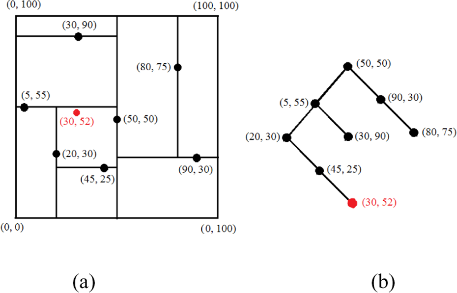
(a) Divided hyperrectangles of the feature space. (b) The standard 2-D tree built by the seven test features.

Priority k-d tree search algorithm

The priority search improved the standard k-d tree search. ^15,16 The priority search is an efficient algorithm, using a sorted list to store subtrees (branches of the tree). When the priority search descends and reaches a subtree, the sibling of the subtree is added to the sorted list. The subtrees in the sorted list are stored in the increasing order of distance between the query feature and the hyperrectangle corresponding to the subtree. Therefore, the sorted list is updated when the priority search descends. The subtree with nearest distance is prior to be examined. The priority search only examines the subtrees stored in the sorted list.

The key steps of the priority search can be summarized as follows ¹⁶ :

Step 1: Apply branch-and-bound search in the descending down k-d tree (or subtree) and ceaselessly update the sorted list, until reaching a leaf node.

Step 2: If the candidate NN of the query feature is null or the distance from the query feature to the candidate is greater than that to the leaf node, the leaf node is treated as the candidate.

Step 3: If the sorted list is empty, stop the program.

Step 4: Extract the subtree with highest priority from the sorted list.

Step 5: If the distance from the query feature to the candidate is smaller than the distance to the hyperrectangle responding to the subtree, stop the program.

Step 6: If the distance from the query feature to the candidate is smaller than the distance to the subtree’s father, turn to step 1.

Step 7: The candidate’s father node is treated as the candidate, and turn to step 1.

In every process of examining a subtree, only one leaf node is reached, so the capacity of the sorted list is equal to the number of the reached leaf nodes and is denoted as E_max. If E_max is small, a few of subtrees are examined, and the NN can be quickly returned, the probability of the NN being exact is low. When E_max is great, the probability of the NN being exact is high, but many subtrees need to be examined, and the algorithm costs more time. Therefore, the parameter E_max is a factor that significantly affects the performance of the priority search. From the aforementioned analysis, we can see that the fundamental reason why the priority search is an efficient and approximate NN algorithm is that the NN should lie in the nearest bins (hyperrectangles) from query feature with high probability and the algorithm limits the number of the reached leaf nodes.

BSFM algorithms

Scale-invariant feature transform

SIFT is an algorithm in computer vision to detect and describe local features in images. The algorithm was proposed by Lowe in 1999. ²⁵ It has been widely used in the field of image processing, including object recognition, robotic mapping and navigation, image stitching, 3-D modeling, gesture recognition, video tracking, individual identification of wildlife, and match moving.

BSFM algorithm

In this section, we introduce the details of the proposed BSFM algorithm, which is illustrated in Figure 2. Before the SIFT features are matched, we extract two SIFT feature sets S1 and S2 of two images I1 and I2 and build two k-d trees kdT1 and kdT2, respectively, based on their feature sets S1 and S2. The BSFM algorithm consists of two key steps. The first step is to find the feature closestT′ from kdT1, which is the closest neighbor of T by the priority search. The second step is to find the feature closestT″ from kdT2, which is the closest neighbor of closestT′ by the priority search. Finally, compare T with closestT″. If they are the same, closestT′ is the correct match feature for T, or else T is given up.

Figure 2.

Two key steps of the BSFM algorithm. BSFM: bidirectional SIFT feature matching; SIFT: scale-invariant feature transform.

The following is the procedure of the BSFM algorithm:

Step 1: Take a SIFT feature T from S2.

Step 2: Find the closest neighbor closestT′ of T by the priority search from kdT1.

Step 3: Find the closest neighbor closestT″ of closestT′ by the priority search from kdT2.

Step 4: Compare T with closestT″. If they are the same, the match between T and closestT′ is accepted, or else there is not a correct match feature for T.

Step 5: Continue to take another SIFT feature from S2 and turn to step 2, until every SIFT feature in S2 is taken.

According to aforementioned description of the BSFM algorithm, the priority search is used twice.

Two extended BSFM (BSFM1R and BSFM2R) algorithms

Lowe stated that if the ratio of distance of the closest neighbor to distance of the second closest neighbor for each query feature is not greater than 0.8, the match between the closest neighbor and query feature is accepted, otherwise abandoning it. ² Thus, we can discard features that did not have good match to the query feature set. In this section, according to the case of adopting the ratio restriction of distances, we propose two extended bidirectional algorithms based on the BSFM algorithm. In one extended bidirectional algorithm, which is called the “BSFM1R algorithm,” the ratio restriction of distances is adopted just in the first step. In the second extended bidirectional algorithm, which is called the “BSFM2R algorithm,” the ratio restriction of distances is adopted in both the first and second steps.

The procedure of the BSFM1R algorithm is as follows:

Step 1: Take a SIFT feature T from S2.

Step 2: Find the closest neighbor closestT′ and second closest neighbor seclosestT′ of T by the priority search from kdT1.

Step 3: If the ratio of distance of closestT′ to distance of seclosestT′ for T is greater than 0.8, there is not a correct match feature for T and turn to step 6.

Step 4: Find the closest neighbor closestT″ of closestT′ by the priority search from kdT2.

Step 5: Compare T with closestT″. If they are the same, the match between T and closestT′ is accepted, or else there is not a correct match feature for T.

Step 6: Continue to take another SIFT feature from S2 and turn to step 2, until every SIFT feature in S2 is taken.

The following is the procedure of the BSFM2R algorithm:

Step 1: Take a SIFT feature T from S2.

Step 2: Find the closest neighbor closestT′ and second closest neighbor seclosestT′ of T by the priority search from kdT1.

Step 3: If the ratio of distance of closestT′ to distance of seclosestT′ for T is greater than 0.8, there is not a correct match feature for T and turn to step 7.

Step 4: Find the closest neighbor closestT″ and second closest neighbor seclosestT″ of closestT′ by the priority search from kdT2.

Step 5: If the ratio of distance of closestT″ to distance of seclosestT″ for closestT′ is greater than 0.8, there is not a correct match feature for T and turn to step 7.

Step 6: Compare T with closestT″. If they are the same, the match between T and closestT′ is accepted, or else there is not a correct match feature for T.

Step 7: Continue to take another SIFT feature from S2 and turn to step 2, until every SIFT feature in S2 is taken.

From the procedures of BSFM, BSFM1R and BSFM2R algorithms, it can be seen that the match between T and closestT′ is just a candidate match after the first step of these three algorithms is processed. We can assert whether or not the candidate match is a correct match, until the second step of them being processed and comparing T and closestT″. If the ratio restriction of distances is adopted in the priority algorithm, the procedure of the priority algorithm is similar to the first step of BSFM1R and BSFM2R algorithms.

Experiments

Experiments on two pairs of images

In this section, we present two group experiments on the basis of two pairs of images, respectively, to compare the matching precisions, recall rates, and speedups of the linear search, the standard search, the priority search, and these three bidirectional algorithms. All the experiments are tested on the Computer of Lenevo (memory: 2Gb, CPU: core i5 2400s), and the test tool was Matlab 2010b.

Figures 3 and 4 show the comparison results of these six algorithms mentioned earlier. In the following, we describe the processes of the first group experiment whose results are shown in Figure 3, which is similar to that in Figure 4. In the first group experiment, the SIFT features of two test images I1 and I2 are matched. I1 is shown in Figure 3(a) and I2 is the image rotated 45° of I1. The size of I1 is 512 × 512 pixels. The k-d trees of the standard search and priority search are built by the SIFT feature set of I1. For every SIFT feature of I2, the linear search would search the closest feature in the SIFT feature set of I1. The first step of these three bidirectional algorithms runs on the k-d tree built by the SIFT feature set of I1 and the second step of them runs on the k-d tree built by the SIFT feature set of I2. The case of adopting the ratio restriction of distances is listed in Table 1, where “Y” means that the ratio restriction of distances is adopted and “N” means that the ratio restriction of distances is not adopted.

Figure 3.

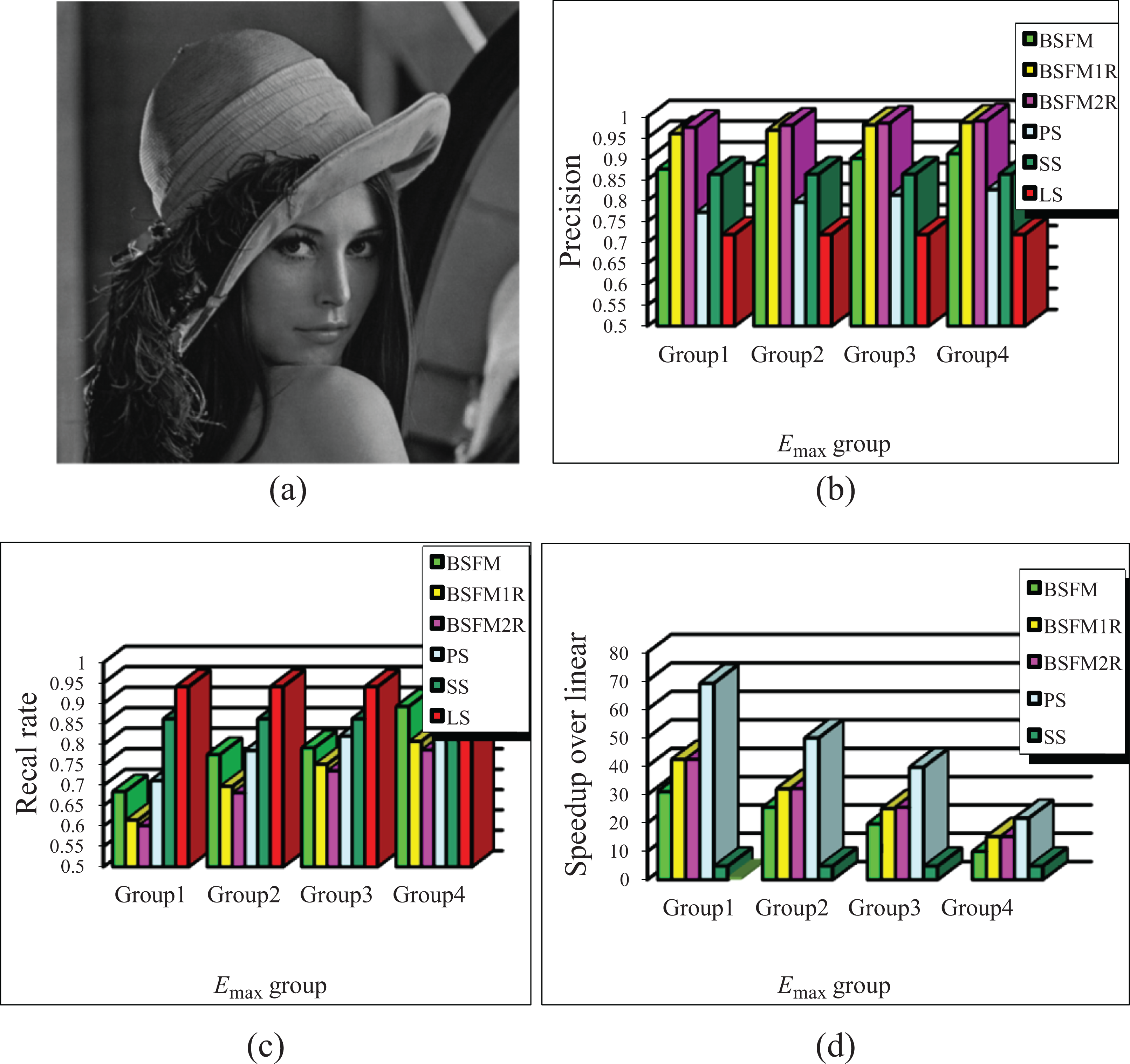
Performance of six algorithms on the basis of I1 and I2. (a) Test image I1; (b) precision; (c) recall rate; (d) speedup over linear search. PS: priority search; SS: standard search; LS: linear search.

Figure 4.

Performance of six algorithms on the basis of I3 and I4. (a) Test image I3; (b) precision; (c) recall rate; (d) speedup over linear search. PS: priority search; SS: standard search; LS: linear search.

Table 1.

The case of adopting the ratio restriction of distances in six algorithms or their key steps.

Algorithm or its key steps	Linear search	Standard search	Priority search	BSFM		BSFM1R		BSFM2R
				Step 1	Step 2	Step 1	Step 2	Step 1	Step 2
Adopting the ratio restriction of distances	Y	Y	Y	N	N	Y	N	Y	Y

BSFM: bidirectional SIFT feature matching; SIFT: scale-invariant feature transform.

The recall rate results of these six algorithms are illustrated in Figures 3(c) and 4(c). The precision of the linear search is the lowest, and inversely the recall rate of the linear search is the biggest. As the E_max increases, the recall rate of the priority search becomes closer to the recall rate of the standard search. That is because, the recall rate of the priority search becomes greater with the increasing of E_max, and the priority search is an algorithm based on the standard search. The recall rates of BSFM1R and BSFM2R algorithms are lower than the recall rate of the priority search, because the first step of BSFM1R and BSFM2R algorithms is similar to the procedure of the priority search, and these two extended algorithms have one more step than the priority search to judge whether or not the candidate match in the first step is correct. The recall rate of the BSFM algorithm is higher than that of the priority search when E_max are in group 4. The main difference between the BSFM algorithm and the priority search is that both of two steps in the BSFM algorithm do not adopt the ratio restriction of distances, but the priority search adopts. It indicates that because of adopting the ratio restriction of distances in the priority search, a few of correct matches can be discarded. Since the frequency of adopting the ratio restriction of distances in BSFM, BSFM1R, and BSFM2R algorithms increases, their recall rates consecutively become low.

The speedups of the standard search, the priority search, and these three bidirectional algorithms over the linear search are illustrated in Figures 3(d) and 4(d). As it can be seen in these two figures, the priority search has the greatest speedup, and the speedup of the standard search is less than 1 and the lowest. That is to say, the time cost of the standard search is higher than other five algorithms on matching SIFT features. It also can be seen that the speedups of the priority search and these three bidirectional algorithms decrease with the increasing of E_max. The speedup of the priority search is almost twice that of the BSFM algorithm, because the priority search must be processed twice in the BSFM algorithm. The speedups of BSFM1R and BSFM2R algorithms are very close and bigger than that of the BSFM algorithm. That is because, if the ratio restriction of distances cannot be satisfied in the first step of BSFM1R and BSFM2R algorithms, the second step of them is not processed.

In order to compare the performances of these six algorithms when the priority search and these three bidirectional algorithms achieve different precisions, four E_max groups are assigned and listed in Tables 2 and 3. If the number of SIFT features is fixed, the precisions achieved by the priority search and these three bidirectional algorithms become higher with the increasing of E_max. In Table 2, the data in the second column are the number of SIFT features and that in the third column is the number of real SIFT feature matches between I1 and I2. The data in the second row are E_max for the priority search and the first step of these three bidirectional algorithms, and the data in the third row are E_max for the second step of these three bidirectional algorithms.

Table 2.

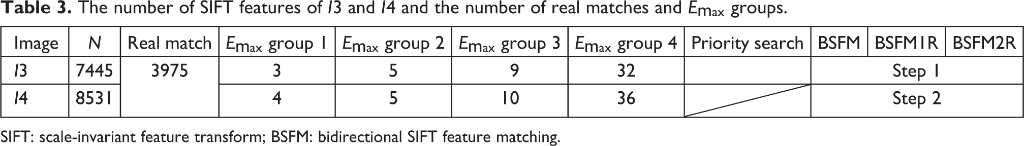
The number of SIFT features of I1 and I2 and the number of real matches and E_max groups.

Image	N	Real match	Emax group 1	Emax group 2	Emax group 3	Emax group 4	Priority search	BSFM	BSFM1R	BSFM2R
I1	3091	1862	2	4	6	15		Step 1
I2	4120		3	4	7	19		Step 2

SIFT: scale-invariant feature transform; BSFM: bidirectional SIFT feature matching.

Table 3.

The number of SIFT features of I3 and I4 and the number of real matches and E_max groups.

Image	N	Real match	Emax group 1	Emax group 2	Emax group 3	Emax group 4	Priority search	BSFM	BSFM1R	BSFM2R
I3	7445	3975	3	5	9	32		Step 1
I4	8531		4	5	10	36		Step 2

SIFT: scale-invariant feature transform; BSFM: bidirectional SIFT feature matching.

The precisions obtained by these six algorithms are illustrated in Figures 3 (b) and 4(b). It can be seen that the linear search obtains the lowest precision. The precisions obtained by BSFM1R and BSFM2R algorithms are higher than that obtained by the linear search, the standard search, and the priority search. The precisions of BSFM1R and BSFM2R algorithms are very close and are much greater than that of the BSFM algorithm. The difference among these three bidirectional algorithms is that the first step of BSFM1R and BSFM2R algorithms adopts the ratio restriction of distances, but the first step of the BSFM algorithm does not adopt. It indicates that in BSFM1R and BSFM2R algorithms, most of false matches are cut down in the first step and only a little of false matches are discarded in the second step.

For these three bidirectional algorithms, if E_max is fixed, the frequency of adopting the ratio restriction of distances will be high, and the precisions become higher and the recall rates smaller. It exhibits the special function of the ratio restriction of distances. Plenty of false matches can be eliminated and a few of correct matches also can be discarded by the ratio restriction of distances. This result is consistent with the theory stated in the research by Lowe. ²

From the results of two group experiments, we can obtain the following conclusions. The precisions of BSFM1R and BSFM2R algorithms are the highest and very close, and the recall rates of them are the lowest. The precision of the linear search is the lowest, and inversely its recall rate is the greatest. The recall rate of the BSFM algorithm is higher than that of the priority search when E_max is large enough. The speedup of the standard search is the lowest, and the speedup of the priority search is almost twice that of the BSFM algorithm. The speedups of BSFM1R and BSFM2R algorithms are very close and greater than that of the BSFM algorithm. When the parameter E_max increases, the precisions and recall rates of the priority search and these three bidirectional algorithms increase, but the speedups of them decrease.

Experiments on two groups of images

The experiments in section “Experiments on two pairs of images” are only with two pairs of images. In order to substantially verify the results obtained in section “Experiments on two pairs of images,” in this section, we do experiments with two image groups. The number of each image group is 100. The images in the first group are not transformed, and the images in the second group are of rotating 45° of the first group images. Extracting the SIFT features of the two group images, each image is corresponding to a SIFT feature set, so there are 100 pairs of SIFT feature sets matched by these six algorithms.

In order to compare the performances of these six algorithms when they achieve low or high precisions, E_max assigned for the priority search and the two steps of these three bidirectional algorithms are illustrated, respectively, in Figure 5, where the curve marked 2 is for the case of achieving low precisions and the curve marked 1 is for high precisions. The processes of these six algorithms in these experiments are specified in the flowing. The k-d trees of the standard search and priority search are built by the feature sets of the images in the first group. For every SIFT feature of the images in the second group, the linear search would search the closest feature in the SIFT feature sets of the images in the first group. The first and second steps of these three bidirectional algorithms run on the k-d trees built by the SIFT feature sets of the images in the first and the second groups, respectively. The case of adopting the ratio restriction of distances is listed in Table 1.

Figure 5.

Curves of E_max values with respect to SIFT feature number. SIFT: scale-invariant feature transform.

There is an example to illustrate how to assign E_max for the priority search and the two steps of these three bidirectional algorithms. Suppose that an image I is in the first group and its rotated image is I′ in the second group, then the number of SIFT features of I and I′ is 2000 and 3000, respectively. For the case of achieving low precisions, refer to the curve marked 2 in Figure 5, the value of E_max is 5 for the priority search and the first step of these three bidirectional algorithms, and 6 for the second step of these three bidirectional algorithms. For the case of achieving high precisions, refer to the curve marked 1 in Figure 5, the value of E_max is 12 for the priority search and the first step of these three bidirectional algorithms, and 15 for the second step of these three bidirectional algorithms.

The performances of these six algorithms running on two image groups are illustrated in Figure 6. The precisions achieved by these six algorithms are illustrated in Figure 6(a) and (b). We can see that the precisions of BSFM1R and BSFM2R algorithms are very close and almost of them are greater than 95%. The precision distributions of the BSFM algorithm and the linear search are mainly from 90% to 95%.

Figure 6.

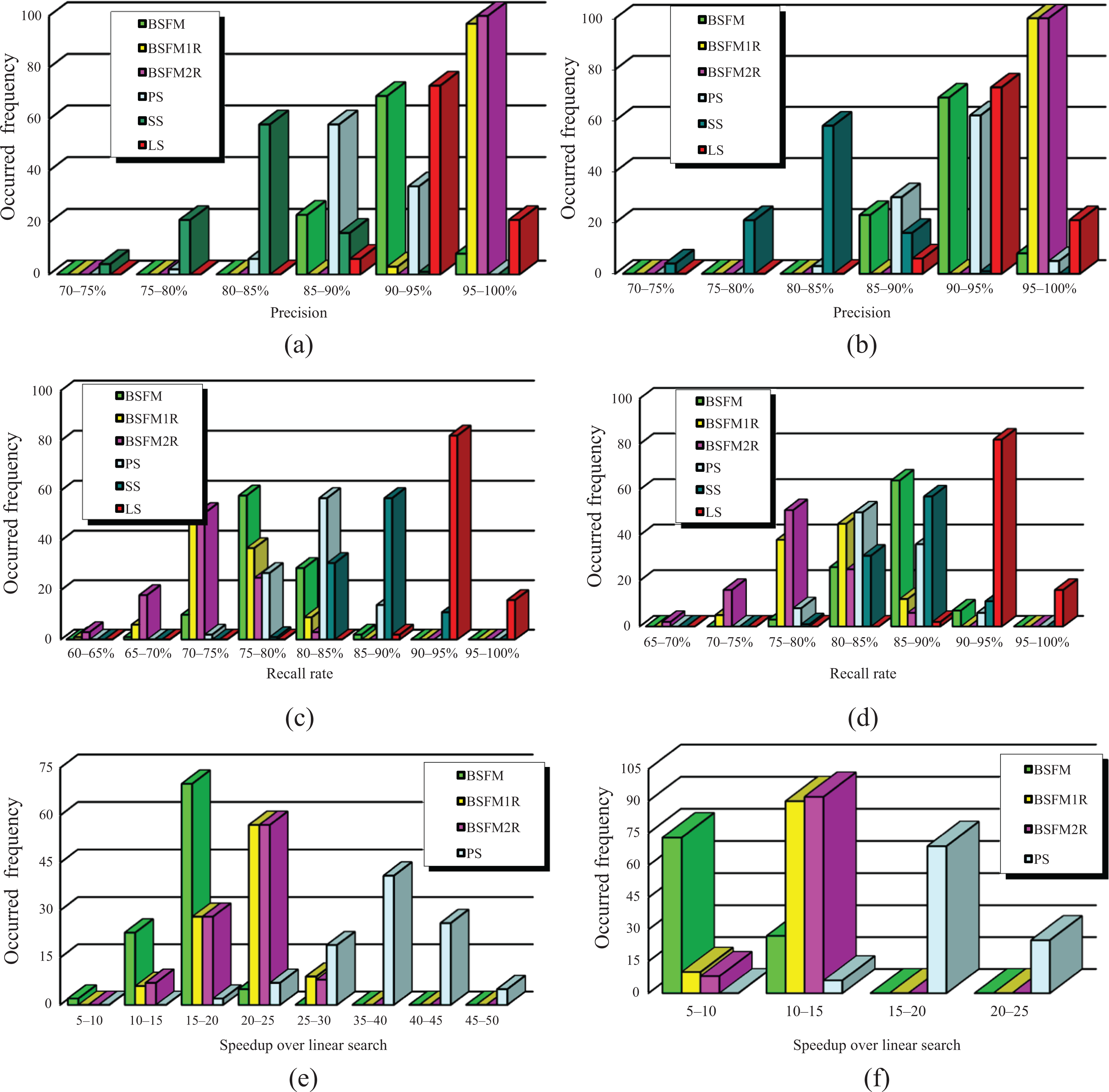
Performance of six algorithms. (a) Precision histogram of six algorithms with E _max referred to the curve marked 2; (b) precision histogram of six algorithms with E _max referred to the curve marked 1; (c) recall rate histogram of six algorithms with E _max referred to the curve marked 2; (d) recall rate histogram of six algorithms with E _max referred to the curve marked 1; (e) speedup histogram of six algorithms with E _max referred to the curve marked 2; (f) speedup histogram of six algorithms with E _max referred to the curve marked 1. PS: priority search; SS: standard search; LS: linear search.

The recall rates achieved by these six algorithms are illustrated in Figure 6(c) and (d). The recall rates of the linear search are the highest, and the recall rate distribution of it is mainly from 90% to 95%. The recall rates of BSFM1R and BSFM2R algorithms are the lowest. The recall rate distribution of the BSFM algorithm in Figure 6(c) is mainly from 75% to 80% and that in Figure 6(d) is mainly from 85% to 90%. Both of the recall rate distributions of the priority search in Figure 6(c) and (d) are mainly from 80% to 85%. It indicates that the recall rate of the BSFM algorithm becomes higher than that of the priority search when E_max is large enough.

The speedups obtained by the priority search and three bidirectional algorithms are illustrated in Figure 6(e) and (f). Because the speedup of the standard search is lower than 1, these two figures do not show it. The speedups of BSFM1R and BSFM2R algorithms are very close and greater than that of the BSFM algorithm. In Figure 6(e), the speedup distribution of the BSFM algorithm is mainly from 15 to 20 and that of the priority search is mainly from 35 to 40. In Figure 6(f), the speedup distribution of the BSFM algorithm is mainly from 5 to 10 and that of the priority is mainly from 15 to 20. It demonstrates that the speedup of the priority search is almost twice that of the BSFM algorithm.

The mean value of the precisions, recall rates, and speedups of these six algorithms in the experiments is calculated and listed in Table 4. The recall rate of the linear search is the highest and that of BSFM1R and BSFM2R algorithms is the lowest. The speedup of the standard search is the smallest and that of the priority search is the greatest. The precisions of BSFM1R and BSFM2R algorithms are the greatest, and the speedups of them are very close and greater than the BSFM algorithm. The parameter E_max in group 2 is bigger than that in group 1. The precisions and recall rates of the priority search and three bidirectional algorithms increase, while the speedups of them decrease, as the parameter E_max becomes larger. To sum up the analyzing results of section Experiments, it comes to the same conclusion.

Table 4.

The mean of the precisions, recall rates, and speedups of six algorithms.

Mean	Linear search	Standard search	Priority search		BSFM		BSFM1R		BSFM2R
			Emax group 1	Emax group 2	Emax group 1	Emax group 2	Emax group 1	Emax group 2	Emax group 1	Emax group 2
Precision	82.01%	93.25%	88.61%	90.78%	91.69%	91.75%	97.40%	97.65%	98.73%	98.92%
Recall rate	93.40%	86.34%	81.57%	84.60%	78.67%	85.95%	74.89%	80.68%	72.88%	78.16%
Speedup over linear search		0.67	32.56	18.36	16.20	9.29	21.09	11.89	21.13	11.96

BSFM: bidirectional SIFT feature matching; SIFT: scale-invariant feature transform.

Processes of different algorithms

In this section, two SIFT feature matching experiments based on Figure 7(a) and (b) are presented. The difference of these two experiments is the process of those six algorithms. The matching results of them are listed. Figure 7(b) is a part of Figure 7(a) and rotated 45°. Figure 7(c) and (d) give the SIFT feature locations.

Figure 7.

Two test images and their SIFT feature locations. (a)I1; (b) I2; (c) SIFT feature locations of I1; (d) SIFT feature locations of I2. SIFT: scale-invariant feature transform.

The processes of these six algorithms in the first experiment are as follows. For every SIFT feature of Figure 7(b), the linear search would search the closest feature in the SIFT feature set of Figure 7(a). The standard search and the priority search run on the k-d tree built by the SIFT feature set of Figure 7(a). The first step of BSFM, BSFM1R, and BSFM2R algorithms runs on the k-d tree built by the SIFT feature set of Figure 7(a), and the second step of them runs on the k-d tree built by the SIFT feature set of Figure 7(b). Figure 8(a) to (f), respectively, illustrate the SIFT feature matching results of the linear search, the standard search, the priority search, and these three bidirectional algorithms.

From Figure 8(a) to (f), it can be seen that the matching number of the linear search is the most. In Figure 8(a) to (c), there are some many-to-one matches, but in Figure 8(d) to (g), there are not many-to-one matches. It demonstrates an important property of these three bidirectional algorithms that they can remove many-to-one matches. From Figure 8(d) to (g), the number of total matches decreases, but the percentage of correct matches increases consecutively. It indicates the special function of the ratio restriction of distances once again.

Figure 8.

SIFT feature matching results of six algorithms based on Figure 7(a) and (b). (a) Linear search; (b) standard search; (c) priority search; (d) BSFM algorithm; (e) BSFM1R algorithm; (f) BSFM2R algorithm. SIFT: scale-invariant feature transform.

The processes of these six algorithms in the second experiment are in the following and different to that in the first experiment. The matching results are, respectively, illustrated in Figure 9. For every SIFT feature of Figure 7(a), the linear search would search the closest feature in the SIFT feature set of Figure 7(b). The matching result of the linear search is illustrated in Figure 9(a). The standard search and the priority search run on the k-d tree built by the SIFT feature set of Figure 7(b) and their matching results are illustrated in Figure 9(b) and (c). The first step of these three bidirectional algorithms runs on the k-d tree built by the SIFT feature set of Figure 7(b), and the second step of them runs on the k-d tree built by the SIFT feature set of Figure 7(a). Their matching results are illustrated in Figure 9(d) to (f).

Figure 9.

Another SIFT feature matching results of six algorithms based on Figure 7(a) and (b). (a) Linear search; (b) standard search; (c) priority search; (d) BSFM algorithm; (e) BSFM1R algorithm; (f) BSFM1R algorithm. SIFT: scale-invariant feature transform.

It can be seen that the results illustrated in Figure 9(a) to (c) are different from the results illustrated in Figure 8(a) to (c). However, the results illustrated in Figure 9(d) to (f) are similar to the results illustrated in Figure 8(d) to (f), respectively. It indicates another property of these three bidirectional algorithms. These three bidirectional algorithms can always obtain the respective same matching results that are not relevant to their processes. But the results of the linear search, the standard search, and the priority search are relevant to their processes.

Conclusion

In order to improve SIFT feature matching precision in image registration, we propose BSFM, BSFM1R, and BSFM2R algorithms based on the priority search. The precisions of BSFM1R and BSFM2R algorithms are very close and higher than that of the linear search, the standard search, the priority search, and the BSFM algorithm. The recall rate of the BSFM algorithm is higher than that of the priority search when E_max is large enough. The speedup of the priority search is almost twice that of the BSFM algorithm. The speedups of BSFM1R and BSFM2R algorithms are very close and greater than that of the BSFM algorithm. When the parameter E_max increases, the precisions and recall rates of the priority search and these three bidirectional algorithms increase, but the speedups of them decrease. There are two special properties of BSFM, BSFM1R, and BSFM2R algorithms, one is that they can remove many-to-one matches and another is that they can always obtain the respective same matching results that are not relevant to their processes.

In image registration, the BSFM1R or BSFM2R algorithm is recommended to match SIFT features. They can achieve not only greater precisions than the linear search, the standard search, the priority search, and the BSFM algorithm but also higher speedups than the BSFM algorithm. In addition, the number of their correct matches can satisfy the requirement of aligning images absolutely.

The idea of utilizing the feature matching algorithm twice is significant, and it can be applied in other domains concerned with searching element matches between two sets.