Sage Journals: Discover world-class research

Abstract

This article proposes a novel advanced differential evolution method which combines the differential evolution with the modified back-propagation algorithm. This new proposed approach is applied to train an adaptive enhanced neural model for approximating the inverse model of the industrial robot arm. Experimental results demonstrate that the proposed modeling procedure using the new identification approach obtains better convergence and more precision than the traditional back-propagation method or the lonely differential evolution approach. Furthermore, the inverse model of the industrial robot arm using the adaptive enhanced neural model performs outstanding results.

Keywords

Advanced differential evolution adaptive neural networks model robot arm modified back-propagation algorithm nonlinear system identification autoregressive with exogenous input model

Introduction

According to recent studies, the differential evolution (DE) algorithm is promising for identifying and controlling nonlinear dynamic system. The first study on DE algorithm is introduced by Storn and Price.¹ Because DE technique possesses several advantages such as simple implementation, good performance, global optimization, and low space complexity, it is one of the most powerful stochastic population-based optimization algorithms. Ilonen et al.² applied the DE algorithm to train feed-forward neural model. This study used DE to find the global optimum for the objective function. In comparison to gradient descent method, we see that DE technique can be applied efficiently for learning neural-based models. The DE-trained neural networks for nonlinear dynamic system identification are introduced in the literatures^3–5 The DE-based trained neural models for controlling nonlinear dynamic systems are presented in the studies by Chen and Yang and Lu et al.^6,7

Anh and Nam⁸ proposed a robot manipulator identification method using a neural multiple-input and multiple-output (MIMO) nonlinear autoregressive exogenous model (NARX) model based on BP algorithm. This study uses BP algorithm to optimally produce the weighting values of neural model. Simulation results demonstrate that the identification of quality based on the proposed neural model and trained by BP algorithm performed well. Alavandar and Nigam⁹ presented the inverse model of the robot arm identification using an adaptive neuro-fuzzy inference system (ANFIS) model. The BP algorithm is used to train the ANFIS model. The identification process based on the experimental training data of inverse kinematics solution and mean squared error (MSE) criterion. The disadvantage of these results relates to the fact that identification process is sometimes trapped in local optimum solution.

Bandurski and Kwedlo¹⁰ introduced a new way to train neural model using the combination of DE technique with a specific gradient descent approach. The steps of mutation and recombination, in each iteration, produce a new agent. This novel agent is adaptively trained by the gradient descent approach before being transferred to the next iteration. The results prove that the proposed algorithm has better selection than the DE or other gradient descent methods. Based on the above analysis, we see that the multilayer perceptron neural networks (MLPNNs) are usually trained by the gradient descent methods (such as BP algorithm, Levenberg Marquardt algorithm). But, these training algorithms achieve the slow convergence speed and the objective function may lead to local minima.

In this article, a new adaptive neural MIMO NARX model was proposed based on an advanced DE (advanced differential evolution (ADE)-AMNM) for inverse model of the three degree of freedom (3-DOF) industrial robot arm identification. This new advanced DE approach links between the DE with the modified back-propagation (MBP) algorithm which is applied to optimally produce the weighting values of neural model. This new advanced method realizes quicker convergence and better accuracy than the traditional BP algorithm or the lonely DE algorithm. So, the proposed adaptive neural MIMO NARX model using the advanced DE algorithm (ADE-AMNM) for inverse kinematics of the robot arm identification approach successfully modeled and performed well.

This article is structured as follows. Section “The inverse model of the 3-DOF industrial robot manipulator” presented the inverse model of the 3-DOF industrial robot arm. Section “An advanced adaptive neural model for nonlinear MIMO system identification” presents the proposed adaptive neural network model for nonlinear system identification. Section “Modeling and identification results” presented identification results. Final section is the conclusion.

The inverse model of the 3-DOF industrial robot manipulator

In general, there are two alternatives, one is to consider the dynamic model^11,12 of the robotic arm and the other is to use the inverse kinematics. The inverse kinematics plays an important role for robot control implementation. The inverse model helps to calculate the needed joint angles from reference trajectory of the end effector. There are various methods to calculate the inverse kinematics results, for example, the algebraic and the geometric method. This article applies the algebraic method to determine the inverse model of the 3-DOF industrial robot arm presented in Figure 1.

Figure 1.

The investigated 3-DOF industrial robot arm. 3-DOF: three degree of freedom.

Using the D-H procedure, we obtain the transformation matrices

H_{0}^{1} = [\begin{matrix} C_{1} & 0 & S_{1} & 0 \\ S_{1} & 0 & - C_{1} & 0 \\ 0 & 1 & 0 & d_{1} \\ 0 & 0 & 0 & 1 \end{matrix}], H_{1}^{2} = [\begin{matrix} C_{2} & - S_{2} & 0 & a_{2} C_{2} \\ S_{2} & C_{2} & 0 & a_{2} S_{2} \\ 0 & 0 & 1 & 0 \\ 0 & 0 & 0 & 1 \end{matrix}], and H_{2}^{3} = [\begin{matrix} C_{3} & - S_{3} & 0 & a_{3} C_{3} \\ S_{3} & C_{3} & 0 & a_{3} S_{3} \\ 0 & 0 & 1 & 0 \\ 0 & 0 & 0 & 1 \end{matrix}]

Therefore, the forward kinematics for a 3-link robot manipulator is given by

H_{0}^{3} = H_{0}^{1} H_{1}^{2} H_{2}^{3} = [\begin{matrix} C_{1} C_{23} & - C_{1} S_{23} & S_{1} & C_{1} (a_{2} C_{2} + a_{3} C_{23}) \\ S_{1} C_{23} & - S_{1} S_{23} & - C_{1} & S_{1} (a_{2} C_{2} + a_{3} C_{23}) \\ S_{23} & C_{23} & 1 & a_{2} S_{2} + a_{3} S_{3} + d_{1} \\ 0 & 0 & 0 & 1 \end{matrix}]

Where, S₁, C₁, S₂, C₂, S₂₃, and C₂₃ represent $sin θ_{1}, cos θ_{1}, sin θ_{2}, cos θ_{2}, sin (θ_{2} + θ_{3}), and cos (θ_{2} + θ_{3})$ , respectively.

A point P represents a given position of the end effector, which can be expressed by

P = [\begin{matrix} C_{1} (a_{2} C_{2} + a_{3} C_{23}) \\ S_{1} (a_{2} C_{2} + a_{3} C_{23}) \\ a_{2} S_{2} + a_{3} S_{23} + d_{1} \end{matrix}] or {\begin{cases} P_{x} = C_{1} (a_{2} C_{2} + a_{3} C_{23}) (2) \\ P_{y} = S_{1} (a_{2} C_{2} + a_{3} C_{23}) (3) \\ P_{z} = a_{2} S_{2} + a_{3} S_{23} + d_{1} (4) \end{cases}

For the typical position solution of the 3-DOF industrial robot arm, the inherent relation of the joint angles θ₁, θ₂, and θ₃ will be presented. First, (2) and (3) are multiplied by S₁ and C₁, respectively

S_{1} C_{1} (a_{2} C_{2} + a_{3} C_{23}) = P_{x} S_{1}

C_{1} S_{1} (a_{2} C_{2} + a_{3} C_{23}) = P_{y} C_{1}

Then,

P_{y} C_{1} - P_{x} S_{1} = 0

Therefore, the necessary result to the joint variable θ₁ is determined by

θ_{1}^{(1)} = A tan 2 (P_{y}, P_{x})

θ_{1}^{(2)} = A tan 2 (- P_{y}, - P_{x}) = π + θ_{1}^{(1)}

Second, in order to calculate θ₃, equations (2) and (3) are multiplied by C₁ and S₁, respectively

C_{1}^{2} (a_{2} C_{2} + a_{3} C_{23}) = P_{x} C_{1}

S_{1}^{2} (a_{2} C_{2} + a_{3} C_{23}) = P_{y} S_{1}

Then

a_{2} C_{2} + a_{3} C_{23} = P_{x} C_{1} + P_{y} S_{1}

Also, equation (4) can be written as follows

a_{2} S_{2} + a_{3} S_{3} = P_{z} - d_{1}

From equations (10), (11), (12) and (13), we obtain

cos θ_{3} = \frac{P_{x}^{2} + P_{y}^{2} + {(P_{z} - d)}^{2} - a_{2}^{2} - a_{3}^{2}}{2 a_{2} a_{3}} = κ

Therefore, the necessary result to the joint variable θ₃ is determined by

θ_{3}^{(1)} = A tan 2 (\sqrt{1 - κ^{2}}, κ)

θ_{3}^{(2)} = A tan 2 (- \sqrt{1 - κ^{2}}, κ)

Finally, in order to find θ₂, equations (12) and (13) can be written as:

(a_{2} + a_{3} C_{3}) C_{2} - (a_{3} S_{3}) S_{2} = P_{x} C_{1} + P_{y} S_{1}

(a_{2} + a_{3} C_{3}) S_{2} + (a_{3} S_{3}) C_{2} = P_{z} - d_{1}

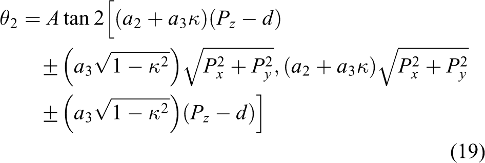
It is clear that $θ_{3}^{(1)}$ and $θ_{3}^{(2)}$ are decoupled of $θ_{1}^{(1)}$ and $θ_{1}^{(2)}$ . Based on equations (17) and (18), θ₂ has the four possible expressions as follows:

θ_{2} = A tan 2 [(a_{2} + a_{3} κ) (P_{z} - d) \pm (a_{3} \sqrt{1 - κ^{2}}) \sqrt{P_{x}^{2} + P_{y}^{2}}, (a_{2} + a_{3} κ) \sqrt{P_{x}^{2} + P_{y}^{2}} \pm (a_{3} \sqrt{1 - κ^{2}}) (P_{z} - d)]

Hence, there will be four different solutions available for the inverse model of the 3-DOF industrial robot arm. In this study, the elbow up set and the shoulder wrist not flipped structure are applied. Then, the inverse model of the investigated 3-DOF robot arm is calculated with

θ_{1} = θ_{1}^{(1)}, θ_{3} = θ_{3}^{(1)}

θ_{2} = A tan 2 [(a_{2} + a_{3} κ) (P_{z} - d) - (a_{3} \sqrt{1 - κ^{2}}) \sqrt{P_{x}^{2} + P_{y}^{2}}, (a_{2} + a_{3} κ) \sqrt{P_{x}^{2} + P_{y}^{2}} + (a_{3} \sqrt{1 - κ^{2}}) (P_{z} - d)]

In summary, the inverse kinematics helps to calculate the needed joint angles $(θ_{1}, θ_{2}, θ_{3})$ from reference position of the end effector (x, y, z). The proposed adaptive neural model optimized by novel advanced DE algorithm (ADE-AMNM) is successfully applied to approximate the needed joint angle values $(θ_{1}, θ_{2}, θ_{3})$ . Specific parameters of the 3-DOF industrial robot arm are tabulated in Table 1.

Table 1.

Specific parameters of the 3-DOF industrial robot arm.

Link	$θ_{i} (degree)$	$a_{i} (mm)$	$α_{i} (degree)$	$d_{i} (mm)$
1	θ ₁	0	90°	d ₁
2	θ ₂	a ₂	0	0
3	θ ₃	a ₃	0	0

3-DOF: three degree of freedom.

An advanced adaptive neural model for nonlinear MIMO system identification

Now, an advanced adaptive neural model (ADE-AMNM) is used to identify the nonlinear system. The AMNM structure is implemented by linking the three-layer MLPNN structure and the ARX model. The AMNM structure has many strongly approximating characteristics of the MLPNN structure and powerful predictive feature of the ARX structure. The block diagram of the proposed AMNM structure is described in Figure 2.

Figure 2.

Block diagram of nonlinear MIMO system identification based on an adaptive neural model. MIMO: multiple-input and multiple-output.

In Figure 2, $u (t) = [u_{1} (t), u_{2} (t), ..., u_{n} (t)]$ is the input signal vector of the nonlinear system and $y (t) = [y_{1} (t), y_{2} (t), ..., y_{m} (t)]$ is the measured output signal vector of the nonlinear system.

To assess the data and identify a model, first, a discrete-time ARX (autoregression with exogenous input) model which performs a relationship between u(t) and y(t) was created. The estimation of the ARX model is the most efficient prediction method. In other words, the ARX model always satisfies the global minimum of the cost function. The ARX model structure with noise input is depicted as follows

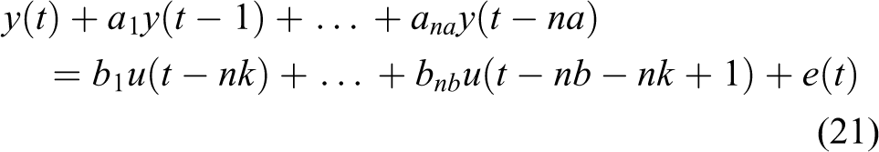
y (t) + a_{1} y (t - 1) + … + a_{n a} y (t - n a) = b_{1} u (t - n k) + … + b_{n b} u (t - n b - n k + 1) + e (t)

Where, e(t) is the white noise measurement, na is the past outputs used for determining the prediction, nb is the past inputs used for determining the prediction, and nk is a time delay (usually 1).

If we let

θ = {[a_{1} a_{2} … a_{n a} b_{1} … b_{n b}]}^{T}

A (q) = 1 + a_{1} q^{- 1} + … + a_{n a} q^{- n a}

B (q) = 1 + b_{1} q^{- 1} + … + b_{n b} q^{- n b}

Substituting expression θ, A(q), and B(q) in (22), (23) and (24) into equation (21), we obtain

y (t) = G (q, θ) u (t) + H (q, θ) e (t) where G (q, θ) = \frac{B (q)}{A (q)}, H (q, θ) = \frac{1}{A (q)}

The discrete ARX model in domain z (with the time delay nk = 1) is depicted as

y (z) = G (z, θ) u (z) + H (z, θ) e (z) where G (z, θ) = \frac{B (z)}{A (z)}, H (z, θ) = \frac{1}{A (z)}

Next, we introduce about the MLPNN. The MLPNN structure is a feed-forward artificial neural network which includes many multilayers perceptron. Figure 3 shows a typical three-layer perceptron neural network structure with n neurons of the input layer, q and m neurons in the hidden and the output layers, respectively.

Figure 3.

Structure of three-layer perceptron neural network.

Based on the studies by Rubio and Bordignon and Gomide,^13,14 as illustrated in Figure 3, the prediction output is computed as follows

{\hat{y}}_{i} (v, w) = F_{i} (\sum_{j = 1}^{q} w_{i j} h_{j} (v) + w_{i 0}) = F_{i} (\sum_{j = 0}^{q} w_{i j} f_{i} (\sum_{l = 1}^{m} v_{j l} ϕ_{l} + v_{j 0}) + w_{i 0})

where v and w are weights of hidden layer and output layer, respectively, f is a sigmoid activation function of the hidden layer and F is a linear activation function of the output layer.

The weights θ is an alternative for the weights matrix of v and w. We denote $θ = (w_{1}, w_{2}, ..., w_{D})$ , with D represents the amount of weighting values of the AMNM or sum of the weights matrix v and the weights matrix w. The weight θ is optimally generated by the training process. The training data includes a set of inputs u(t) and an experimental output y(t). The training data is set by

Z^{N} = {[u (t), y (t)] | t = 1, …, N}

The goal of learning process is to fix a mapping between the learning data Z^N and the weights θ of the AMNM structure

Z^{N} \to \hat{θ}

So that the AMNM produces the prediction output $\hat{y} (t)$ as well as possible to the experimental output y(t). The training process is based on mean square error (MSE) criterion. The MSE is depicted as follows

E_{N} (θ, Z^{N}) = \frac{1}{2 N} \sum_{t = 1}^{N} {[y (t) - \hat{y} (t | θ)]}^{T} [y (t) - \hat{y} (t | θ)]

The weights θ are determined as follows

\hat{θ} = \underset{θ}{\arg \min} E_{N} (θ, Z^{N})

There are many differential methods to train the AMNM structure. This article uses the modified MBP algorithm, the DE technique, and the novel advanced DE technique to train the AMNM for approximating the nonlinear dynamic MIMO system. This training method is applied to optimally produce the weighting values θ of AMNM. In the training process, the weights θ are adaptively modified to choose a functional mapping available. The adaptation can be determined by minimizing the objective function E_N which is depicted in equation (30). The prediction output $\hat{y} (t | θ)$ , which is an output of the AMNM, is dependent on the weights θ and input signal u(t).

Adaptive MIMO neural model optimized by back-propagation algorithm

The back-propagation (BP) algorithm is the most popular learning algorithm. It included two steps to transmit the information. The first, the input signal u(t) is transmitted from input layer to output layer of the AMNM structure to create the output signal $\hat{y} (t)$ . The second, an error in the output node is corrected by back propagating this error by adjusting weights through the hidden layer and back to the input layer. Based on Figure 2, the BP algorithm trained the AMNM can be implemented as follows:

Step 1: Setting parameters

We must select the learning rate η > 0, the maximum of MSE E _max, and create training data Z^N , which include K sample $(x (k), d (k)), k = {1, 2, ..., K}$

Step 2: Initiation

We assign MSE E = 0, variable k = 1, and randomly generated the weights of the AMNM $w_{ia} (k), v_{aj} (k)$ . Where, $i = {1, 2, ..., m}, j = {1, 2, ..., n}, and a = {1, 2, ..., q}$ .

Step 3: Compute the output signal of the AMNM $\hat{y} (t)$ (forward propagating)

Hidden layer : n e t_{a} (k) = \sum_{j = 1}^{n} v_{a j} (k) u_{j} (k)

z_{q} (k) = f (n e t_{q} (k))

Output layer : n e t_{i} (k) = \sum_{a = 1}^{q} w_{i a} (k) z_{q} (k)

{\hat{y}}_{i} (k) = F (n e t_{i} (k))

Step 4 Update the weights of the AMNM (back propagating error)

Output layer : δ_{o i} (k) = [d_{i} (k) - {\hat{y}}_{i} (k)] [F^{'} (n e t_{i} (k))]

w_{i a} (k + 1) = w_{i a} (k) + η δ_{o i} (k) z_{q} (k)

Hidden layer : δ_{h a} (k) = [\sum_{i = 1}^{m} δ_{o i} (k) w_{i a} (k)] [f^{'} (n e t_{a} (k))]

v_{a j} (k + 1) = v_{a j} (k) + η δ_{h a} (k) u_{j} (k)

Step 5 Compute the MSE

E = E + \frac{1}{2} \sum_{i = 1}^{m} {(d_{i} (k) - {\hat{y}}_{i} (k))}^{2}

Step 6 $if k<K then k=k+1 and go back to step 3 if k = K then go to step 7$

Step 7: The end of a training cycle

$\begin{array}{l} if E < E_{max} then stopping training \\ if E \geq E_{max} then E =0, k =1 and go back to \\ step 3 to begin a new training cycle \end{array}$

The flowchart of BP algorithm trained an adaptive MIMO neural model is presented in Figure 4.

Figure 4.

Flowchart of BP algorithm trained an adaptive MIMO neural model. BP: back-propagation; MIMO: multiple-input and multiple-output.

Adaptive neural model optimized by ADE approach

The DE technique is initially appeared as a technical report by Storn and Price in 1995. It is one of the most popular and powerful stochastic population based-optimization algorithms in current use. Like other evolutionary algorithms,^15,16 DE strategy and programming can be implemented in Figures 5 and 6.

Figure 5.

Main stages of the DE algorithm. DE: differential evolution.

Figure 6.

Flowchart of DE method trained an adaptive MIMO neural model. DE: differential evolution; MIMO: multiple-input and multiple-output.

Step 1: Initializing parameters

Firstly, it needs to choose the dimension of population (NP), the amount of maximal generation G _max, the mutation rate F, the crossover factor C, and the lower and upper limits for each parameter.

Step 2: Setting population

Produce an initialized population par hazard with NP D-sized vectors

P_{G} = {(θ_{1, G}, θ_{2, G}, …, θ_{N P, G})}^{T}, G = 1, …, G_{max}

θ_{i, G} = (w_{1, i, G}, w_{2, i, G}, …, w_{D, i, G}), i = 1, …, N P

where D represents the amount of weighting values of the AMNM, i denotes an index to the population, and G denotes the number of iterations.

Step 3: Estimating population

Estimate all individuals. If the fitness result of each individual responds to the predefined criteria, keeping this result and STOP. On the contrary, go to step 4.

Step 4: Choosing variables par hazard for the ith individual of population

r_{1}, r_{2}, r_{3} \in [1, 2, ..., N P], except r_{1} \neq r_{2} \neq r_{3} \neq i

Step 5: Realizing the mutation procedure

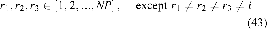
Produce a mutant vector through using mutant operator to every individual as follows

m v_{j, i, G + 1} = w_{j, r_{1}, G} + F (w_{j, r_{2}, G} - w_{j, r_{3}, G}), for j = 1, …, D

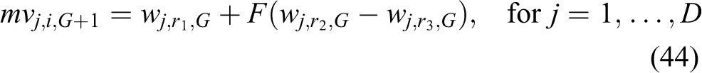
with $F \in (0, 1]$ is the mutant rate.

Step 6: Realizing the crossover/recombination procedure

Create a test vector through relinking the destination vector with the mutant one as follows

t v_{j, i, G + 1} = {\begin{cases} m v_{j, i, G + 1} if r a n d_{j} [0, 1) \leq C \\ w_{j, i, G} otherwise \end{cases}, where C \hat{I} [0, 1)

Step 7 Realizing the selection procedure

Choose between the trial one and the destination vector as follows

θ_{i, G + 1} = {\begin{cases} t v_{i, G + 1} if E_{N} (y, \hat{y} (u, θ_{i, G + 1})) \leq E_{N} (y, \hat{y} (u, θ_{i, G})) \\ θ_{i, G} otherwise \end{cases}

Step 8 Repeating steps 4–7 until ending criteria is satisfied

Adaptive neural model optimized by advanced DE algorithm

System identification using adaptive neural model optimized with MBP method has been regarded as an appropriate approach due to its approximating capability and its identification ability of nonlinear MIMO system. But, the identification process using BP algorithm is sometime trapped in local optimum result. On the other hand, DE technique is recognized as strong global robust optimization with rather low precision. Hence by linking the DE and the MBP algorithm, a novel ADE method is proposed which possesses strong advantages of both DE and MBP algorithm.

There were various methods for using the local search (LS)-based MBP technique inside the global optimization using the ADE approach. In this study, proposed MBP method is used in each test vector—create test vector by linking the destination vector with the mutant one—to create a LS test vector before leaping to step selection procedure. The proposed scheme ADE is summarized in Figure 7.

Figure 7.

Flowchart of proposed ADE algorithm trained an adaptive neural model. ADE: advanced differential evolution.

Modeling and identification results

In this article, the inverse model of the 3-DOF industrial robot arm is investigated. The inverse kinematics is based on kinematics equation of robot to find joint angles $(θ_{1}, θ_{2}, θ_{3}) or (q_{1}, q_{2}, q_{3})$ from specified the position of the end effector $(p_{x}, p_{y}, p_{z})$ with unknown transfer function. The approximation process $(q_{1}, q_{2}, q_{3})$ is appropriate to learning by an adaptive MIMO neural model (AMNM) based on some training algorithm such as BP algorithm, DE, and hybrid DE. Thus, the AMNM structure is created by combining a three-layer MLPNN with a first-order ARX structure. We now describe the block diagram of the inverse kinematics structure of the 3-DOF industrial robot arm identification using the AMNM model presented in Figure 8 as follows,

Figure 8.

Block diagram of the inverse kinematics identification using the AMNM structure.

In general, the procedure of identifying a nonlinear dynamic MIMO system includes four steps as illustrated in Figure 9.

Figure 9.

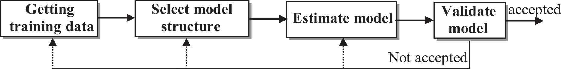
Main stages of the system identification.

Step 1: Selecting learning data

The training data is recorded by the experimental input–output data. This data is determined from the inverse kinematics of the three-link robot manipulator. Where the input values $(p_{x}, p_{y}, p_{z})$ denote the position of the end effector and the output signals $(q_{1}, q_{2}, q_{3})$ are for the joint angles. The process of collecting input–output data of robot manipulator is depicted in Figure 10.

Figure 10.

Collecting input–output data of the 3-DOF industrial robot arm. 3-DOF: three degree of freedom.

The training data includes a set of input signals $u (t) = (p_{x}, p_{y}, p_{z})$ and the experimental output signals $y (t) = (q_{1}, q_{2}, q_{3})$ . The training data is set by

Z^{N} = {[u (t), y (t)] t = 1, …, N}

After running the model in Figure 10, we have input and output signals of the industrial robot manipulator as Figure 11. Where e(t) is a white noise measurement.

Figure 11.

Input–output signal of the 3-DOF industrial robot arm. 3-DOF: three degree of freedom.

Step 2: Select model structure

After having the training data Z^N, the suitable model structure is selected by determining the best networks structure through the given regression as input. This study applies the proposed AMNM model as

Regressive vector

ϕ (t) = {[p_{z} (t - 1) p_{y} (t - 1) p_{x} (t - 1) q_{1} (t - 1) q_{2} (t - 1) q_{3} (t - 1)]}^{T}

Predictive vector

\hat{y} (t | θ) = \hat{y} (t | t - 1, θ) = g (ϕ (t), θ)

with ϕ(t) represents the regression vector, θ denotes the weights vector, and g represents the function operated through the neural model.

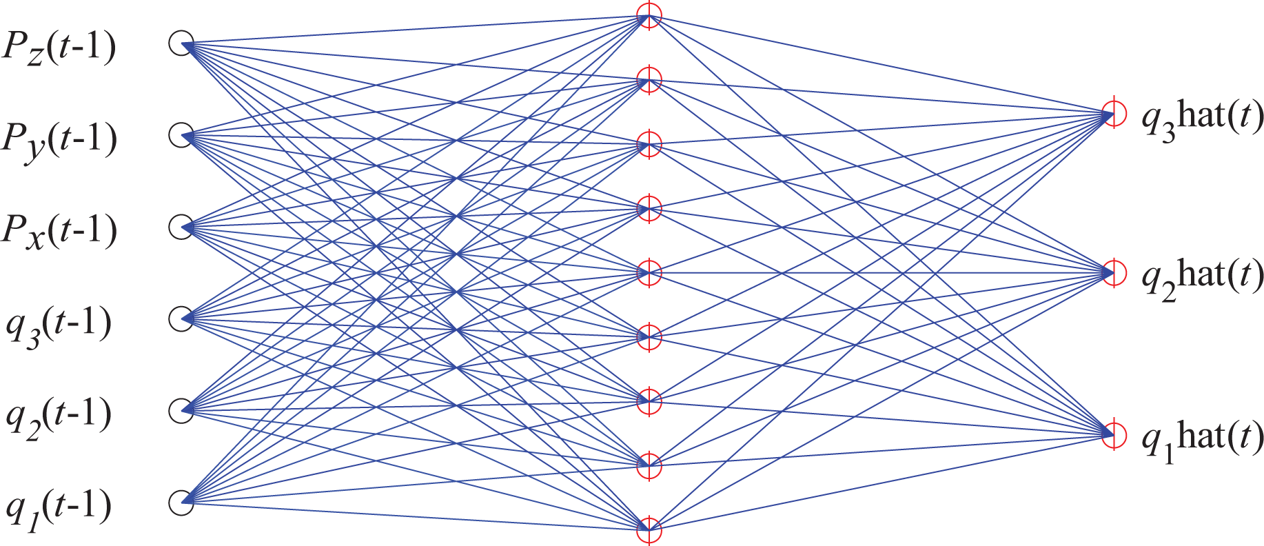
Based on Figure 8, we see that the proposed AMNM structure is created by a fully connected 3-layer feed-forward MLPNN with six inputs, q hidden neurons and three outputs units. Based on the number of hidden layer neuron and training methods, we determine the best result of weights θ.

Step 3: Estimate model

At this step, we solve the optimization problem to find the model parameters by minimizing the objective function E_N . This article uses a BP algorithm, a DE algorithm, and a new hybrid DE algorithm to determine the optimally weights θ.

Thus, the AMNM is estimated or determined the structure of the regression vector.

Step 4: Validate model

This step aims to verify the neural network applying input data sets not used in the evaluating process.¹⁷ The error is once more calculated as abovementioned. If it responds to an appropriate limit, then the investigated network has favorably generalized and can be applied in practice for other real system. The proposed AMNM model is considered to possess the capability of generalization when the input–output relationship collected from the network is approximately correct for input–output patterns never used in the learning process of the investigated model.^18,19

An adaptive neural model (AMNM) optimized by an advanced DE algorithm

First, we selected a number of generations and a number of LS’ iterations to study the performance identification of the AMNM optimized by the proposed ADE algorithm. The AMNM structure with six inputs, five hidden neurons, and three outputs is depicted in Figure 12. Table 2 gives the proposed ADE parameters applied in simulation.

Figure 12.

The AMNM structure with five hidden neurons.

Table 2.

Proposed ADE variables applied in simulation.

Proposed ADE variables	Value
Sampling number (T)	40
Amount of hidden nodes	5
Amount of generations	–
Bounded range of weighting values	[−1 1]
Population dimension (NP)	20
Mutation rate (F)	0.39
Crossover factor (C)	0.36
BP learning rate (η)	0.00009

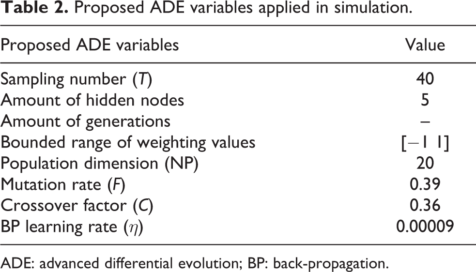
ADE: advanced differential evolution; BP: back-propagation.

Figure 13 shows the fitness convergence of inverse kinematics result of the 3-DOF industrial robot arm using the AMNM model-based hybrid differential evolution (HDE) algorithm. Here, a number of generations are 500 GEN and a number of LS’ iterations is changed from 10 up to 150. Table 3 gives the performance identification in term of time’s convergence and MSE.

Figure 13.

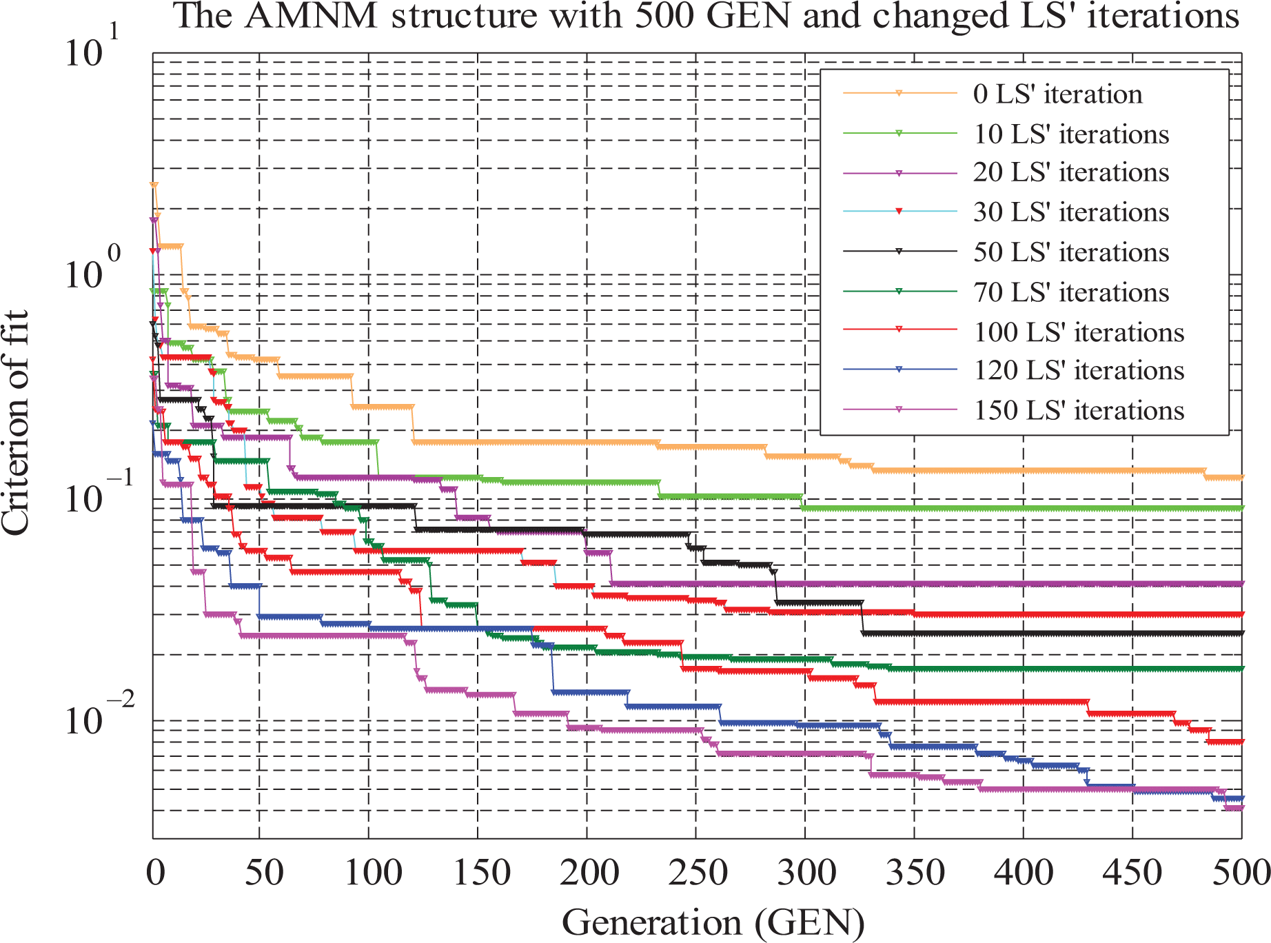
The fitness convergence of inverse kinematics solution using the AMNM with 500GEN. GEN: generation.

Table 3.

The performance identification using the AMNM 500GEN.

LS’ iteration	Time of convergence (s)	MSE
0	1	0.1219
10	4	0.0888
20	8	0.0409
30	11	0.0297
50	16	0.0264
70	22	0.0170
100	32	0.0081
120	40	0.0044
150	50	0.0041

LS: local search; MSE: mean squared error.

Figure 14 shows the fitness convergence of inverse model solution of the 3-DOF industrial robot arm using the AMNM model-based ADE algorithm. Here, a number of generations are 750 GEN and a number of LS’ iterations is changed from 10 to 120 (namely, the AMNM 750GEN). Table 4 gives the performance identification in term of time’s convergence and MSE.

Figure 14.

The fitness convergence of inverse kinematics solution using the AMNM 750GEN. GEN: generation.

Table 4.

The performance of identification procedure using the AMNM 750GEN.

LS’ iteration	Time of convergence (s)	MSE
0	1.5	0.0651
10	6	0.0604
20	12	0.0463
40	20	0.0220
50	26	0.0100
70	34	0.0068
90	49	0.0024
110	54	0.0051
120	56	0.0040

LS: local search; MSE: mean squared error.

Continually, Figure 15 shows the fitness convergence of inverse model solution of the 3-DOF industrial robot arm using the AMNM structure-based ADE algorithm. Here, a number of generations are 1500 GEN and a number of LS’ iterations is changed from 10 to 120 (namely the AMNM 1500 GEN). Table 5 gives the identification performance in term of time’s convergence and MSE.

Figure 15.

The fitness convergence of inverse kinematics solution using the AMNM 1500GEN. GEN: generation.

Table 5.

The performance of identification process using the AMNM 1500GEN.

LS’ iteration	Time of convergence (s)	MSE
0	3	0.0668
10	12	0.0196
20	22	0.0115
40	40	0.0094
50	50	0.0046
70	70	0.0081
90	87	0.0071
100	96	0.0155
120	122	0.0085

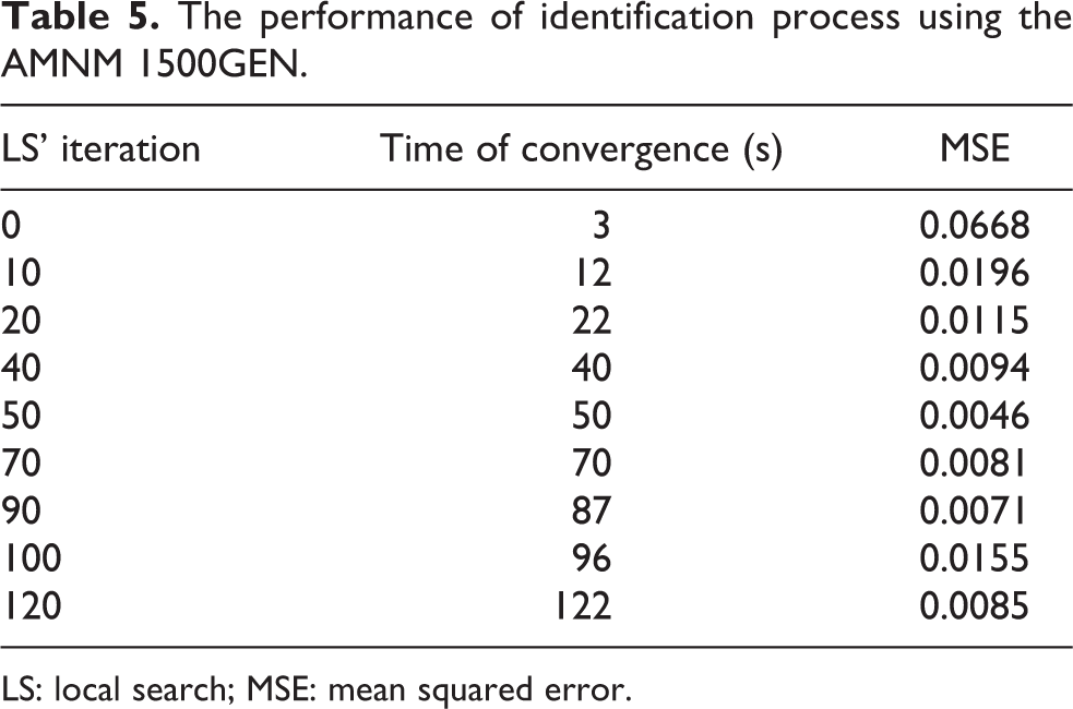
LS: local search; MSE: mean squared error.

Forwardly, Figure 16 introduces the fitness convergence of inverse model solution of the 3-DOF industrial robot arm using the AMNM structure-based ADE algorithm. Here, a number of generations are 3000 GEN and a number of LS’ iterations is changed from 10 to 100 (namely, the AMNM 3000GEN). Table 6 gives the identification performance in term of time’s convergence and MSE.

Figure 16.

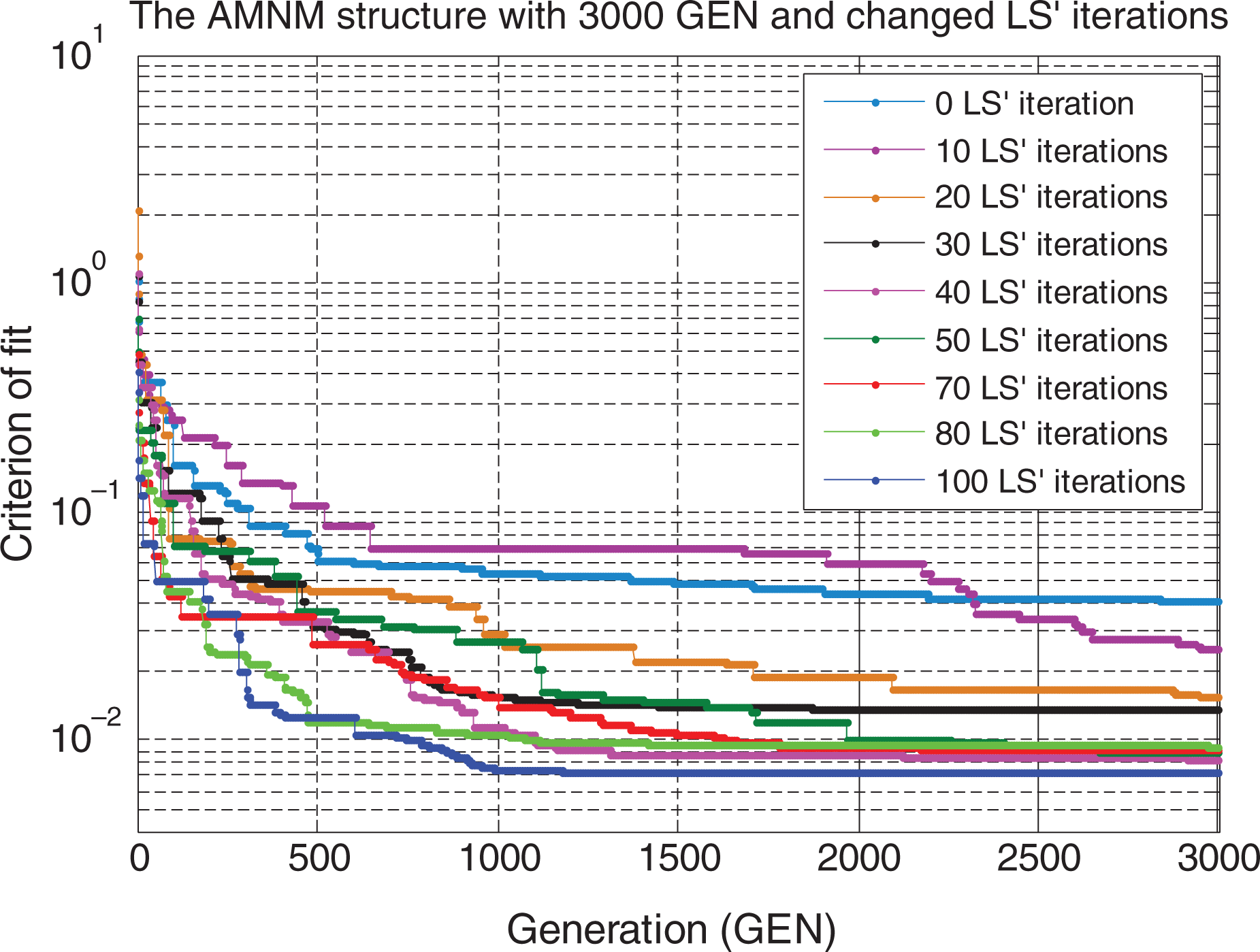
The fitness convergence of inverse kinematics solution using the AMNM 3000GEN. GEN: generation.

Table 6.

The performance of identification process using the AMNM 3000GEN.

LS’ iteration	Time of convergence (s)	MSE
0	5	0.0408
10	25	0.0255
20	45	0.0157
30	60	0.0137
40	83	0.0081
50	100	0.0089
70	135	0.0092
80	157	0.0095
100	191	0.0073

LS: local search; MSE: mean squared error.

Based on these results, we see that the performance of inverse model solution of the 3-DOF industrial robot arm depends on a number of ADE’ generations and a number of LS’ iterations as well. A case of AMNM structure with five hidden layer neurons, 750 GEN and 120 LS’ iteration giving the best MSE value (MSE = 0.0040) and the best time of convergence 56 s which eventually represents the most suitable identification performance.

Next, we change a number of hidden layer neurons to study the performance identification of the proposed the AMNM optimized by ADE technique.^20,21 The AMNM model composes of six inputs and three outputs. The number of hidden neurons is changed between 4 and 10. Other parameters include 750 GEN and 120 LS’ iterations which are applied. The AMNM structure with six inputs, four hidden neurons, and three outputs is depicted in Figure 17. The AMNM structure with six inputs, nine hidden neurons, and three outputs is figured in Figure 18.

Figure 17.

The AMNM structure with four hidden neurons.

Figure 18.

The AMNM structure with nine hidden neurons.

Figure 19 shows the fitness convergence of inverse model solution of the 3-DOF industrial robot arm using the AMNM structure-based ADE algorithm. Here, a number of hidden neurons is changed between 4 and 10. Table 7 gives the performance identification in term of time’s convergence and MSE.

Figure 19.

Comparison on fitness convergence of AMNM when changing number of hidden neurons.

Table 7.

The identification performance with changed amount of hidden nodes.

Amount of hidden nodes	Time of convergence (s)	MSE
4	52	0.0076
5	56	0.0041
6	61	0.0049
7	66	0.0049
8	67	0.0053
9	71	0.0056
10	74	0.0076

LS: local search; MSE: mean squared error.

From the results, it is clear that when we increase the number of hidden layer neurons, the time of convergence increases significantly but the performance of identifying industrial robot manipulator doesn’t change in the same way. The fact is that the sample of AMNM structure with five hidden layer neurons obtains the best MSE value (MSE = 0.0041) in comparison to other samples (with time of convergence 56 s). Eventually, it is concluded that the proposed AMNM structure with five hidden layer neurons optimized with novel ADE identification method keeps the most suitable identification performance.

In summary, the performance of inverse model solution of the 3-DOF industrial robot arm depends on the proposed AMNM structure and ADE’s parameters. The best identified AMNM structure composes of six inputs, five hidden nodes, and three outputs, meanwhile ADE’ variables include NP = 15, F = 0.39, C = 0.36, GEN = 750, and LS’ iterations = 120 which give the most suitable identification performance.

Comparison on the performance identification between BP, DE, and HDE algorithm

To assess the quality of the inverse model solution for the 3-DOF industrial robot arm based on the AMNM structure optimized by a new advanced ADE technique, we should make comparison with traditional methods such as BP and DE algorithms. ^22,23,24

Figure 20 shows the comparison results of the identification quality of inverse model solution for the 3-DOF industrial robot arm using the AMNM structure which is trained and optimally minimized by BP, DE, and ADE algorithms. Figure 21 presents the comparative results on fitness convergence of inverse model solution for the 3-DOF industrial robot arm based on the AMNM structure-based MBP, DE, and proposed ADE algorithm. Table 8 gives the performance of identification process in term of time’s convergence and MSE.

Figure 20.

Comparative study on the identification quality using the AMNM-based BP, DE, and ADE. ADE: advanced differential evolution; BP: back-propagation; DE: differential evolution.

Figure 21.

Comparison on the fitness convergence for three methods.

Table 8.

The identification performance based on the new AMNM optimized by MBP, DE, and proposed ADE.

Method	Time of convergence (s)	MSE
BP-AMNM	2	0.0828
DE-AMNM	1.5	0.0651
ADE-AMNM	56	0.0041

DE: differential evolution; ADE: advanced differential evolution; BP: back-propagation; MBP: modified back-propagation; MSE: mean squared error.

Based on the results above, we see that the inverse model solution of a 3-DOF industrial robot arm using the AMNM structure optimized by a new advanced ADE method obtains a quicker convergence and a better accuracy than the traditional BP technique or the lonely DE method.

Conclusion

This article introduces a new method using an adaptive neural MIMO model (AMNM) combined with a new ADE for the modeling and identification the inverse model of the 3-DOF industrial robot arm. By combining the DE and MBP algorithm, the novel advanced method successfully contains the advantages of both local and global search. The simulation and experiment studies demonstrated that the proposed ADE technique obtained a quicker convergence and a better accuracy than all other identification methods. Hence, this new ADE trained neural network has been regarded as a powerful method in nonlinear multivariable system identification.

Footnotes

Declaration of conflicting interests

The author(s) declared no potential conflicts of interest with respect to the research, authorship, and/or publication of this article.

Funding

The author(s) disclosed receipt of the following financial support for the research, authorship, and/or publication of this article: This article was fully supported by the National Foundation for Science and Technology Development (Vietnam), under grant number MDT: 107.01-2015.23, Vietnam, and the Vietnam National University-Ho Chi Minh City (Vietnam) under grant number B2016-20-03.

References

Storn

Price

. Differential evolution: a simple and efficient adaptive scheme for global optimization over continuous spaces, Technical Report TR-95 -012. Berkeley: International Computer Science Institute, 1995.

Ilonen

Kamarainen

Lampinen

. Differential evolution training algorithm for feed-forward neural networks. Neural Process Lett 2003; 17: 93–105.

Narendra

Parthaasarathy

. Identification and control of dynamical systems using neural networks. IEEE Trans Neural Netw 1990; 1: 4–27.

Kuschewski John

Hui

Zak

. Application of feed-forward neural networks to dynamical system identification and control. IEEE Trans Control Syst Technol 1993; 1: 37–49.

Swayamsiddha

Thethi

. Nonlinear system identification using evolutionary computing based training schemes. In: IJCA Proceedings on international conference on communication, circuits and systems, vol. iC3S(6), 2013, pp. 12–16.

Chen

C-H

Yang

S-Y

. A knowledge-based cooperative differential evolution for neural fuzzy inference systems. Soft Comput 2013; 17: 883–895.

Yang

Liu

. The PID controller based on the artificial neural network and the differential evolution algorithm. J Comput 2012; 7: 2368–2375.

Anh

HPH

Nam

. Novel adaptive forward neural MIMO NARX model for the identification of industrial 3-DOF robot arm kinematics. Int J Adv Robot Syst 2012; 9: 1–12.

Alavandar

Nigam

. Neuro fuzzy based approach for forward kinematics solution of industrial robot manipulators. Commun Control 2008; 3: 224–234.

10.

Bandurski

Kwedlo

. Training neural networks with a hybrid differential evolution algorithm. Informatyka – Zeszyt 2009; Z4: 5–17.

11.

Rubio

Serrano

Figueroa

. Dynamic model with sensor and actuator for an articulated robotic arm. Neural Comput Appl 2014; 24(3–4): 573–581.

12.

Kumar

Panwar

Born

. Adaptive neural controller for space robot systems with an attitude controlled base. Neural Comput Appl 2013; 23(7–8): 2333–2340.

13.

Rubio

. Modified optimal control with a back-propagation network for robotic arms. IET Control Theory Appl 2012(6): 2216–2225.

14.

Bordignon

Gomide

. Uninorm based evolving neural networks and approximation capabilities. Neurocomputing 2014; 127: 13–20.

15.

Rubio

Perez Cruz

. Evolving intelligent system for the modeling of nonlinear systems with dead-zone input. Appl Soft Comput 2014; 14(Part B): 289–304.

16.

Rubio

. Evolving intelligent algorithms for the modeling of brain and eye signals. Appl Soft Comput 2014; 14(Part B): 259–268.

17.

Hieu

Yonggwan

. The use of evolutionary algorithm in training neural networks for hematocrit estimation. In: Pinheiro dos Santos

(ed.) Evolutionary computation. Vienna: INTECH publisher, 2009, pp. 375–385.

18.

Lee

Kuo1

Chang

. Performance enhancement of the differential evolution algorithm using local search and a self-adaptive scaling factor. Int J Innovat Comput Inf Control 2012; 8(4): 2665–2679.

19.

Subudhi

Jena

. Nonlinear system identification using memetic differential evolution trained neural networks. Neurocomputing 2011; 74: 1696–1709.

20.

Roy

Das

Mondal

. Effective system identification using fused network and de based training scheme. IJSCE 2013; 3(3): 105–112.

21.

Lin

C-J

C-F

Lee

C-Y

. Design of recurrent functional neural fuzzy network using modified differential evolution. Int J Innovat Comput Inf Control 2011; 7: 669–683.

22.

Ahma

Raza

. A differential evolution based adaptive neural network pitch controller for a doubly fed wind turbine generator system. Res J Appl Sci Eng Technol 2013: 22(6): 4271–4280.

23.

Panigrahi

Bhoi

Karali

. A modified differential evolution algorithm trained pi-sigma neural network for pattern classification. Int J Soft Comput Eng 2013; 3: 133–136.

24.

Slowik

Bialko

. Training of artificial neural networks using differential evolution algorithm. In: 2008 conference on human system interactions. IEEE, 2008, pp. 60–65.

Robot manipulator identification based on adaptive multiple-input and multiple-output neural model optimized by advanced differential evolution algorithm

Abstract

Keywords

Introduction

The inverse model of the 3-DOF industrial robot manipulator

An advanced adaptive neural model for nonlinear MIMO system identification

Adaptive MIMO neural model optimized by back-propagation algorithm

Adaptive neural model optimized by ADE approach

Adaptive neural model optimized by advanced DE algorithm

Modeling and identification results

An adaptive neural model (AMNM) optimized by an advanced DE algorithm

Comparison on the performance identification between BP, DE, and HDE algorithm

Conclusion

Footnotes

Declaration of conflicting interests

Funding

References