Sage Journals: Discover world-class research

Abstract

Controlling a humanoid robot with its typical many degrees of freedom is a complex task, and many methods have been proposed to solve the problem of humanoid locomotion. In this work, we generate a gait for a Hitec Robonova-I robot using a model-free approach, where fairly simple parameterized models, based on truncated Fourier series, are applied to generate joint angular trajectories. To find a parameter set that generates a fast and stable walk, optimization algorithms were used, specifically a genetic algorithm and particle swarm optimization. The optimization process was done in simulation first, and the learned walk was then adapted to the real robot. The simulated model of the Robonova-I was made using the USARSim simulator, and tests made to evaluate the resulting walks verified that the best walk obtained is faster than the ones publicly available for the Robonova-I. Later, to provide an additional validation, the same process was carried out for the simulated Nao from the RoboCup 3D Soccer Simulation League. Again, the resulting walk was fast and stable, overcoming the speed of the publicly available magma-AF base team.

Keywords

Humanoid robot walk optimization genetic algorithms particle swarm optimization

Introduction

Humanoid robots are claimed to be more adequate than wheeled ones for locomotion in unstructured human environments that include floor discontinuities, ladders, rocks, debris, and so on. However, walk control for humanoid robots (biped locomotion) is a particularly challenging problem, because it encompasses many characteristics acknowledged for making a control problem hard: nonlinearities, underactuation, many degrees of freedom (DOFs), and so forth. As a result, classical control methods fail when applied to biped locomotion. Still, many alternative approaches have been proposed, but so far there is no robot that can walk as well as a human does.

Biped locomotion methods can be grouped into two main approaches: model-based and model-free. Model-based methods depend on analytical models of the dynamics of the robot. Since modeling a high DOF humanoid robot is currently unfeasible, approximate models are used, for example, “3D Linear Inverted Pendulum.”¹ Then, a controller is developed for the model assuming that the dynamics of the robot follows the model. Despite producing incredible results, as the walking performance achieved by the Honda ASIMO robot,² the best model-based walks still operate in a very conservative way and produces very energy inefficient motion.³

On the other hand, model-free methods try to create a controller directly, without a mathematical model for the dynamics of the robot. Two known model-free methods are the central pattern generator (CPG)⁴ and the ballistic walking.⁵ CPG is inspired by nature, where evidence shows that human locomotion is generated by neural networks that produce rhythmic patterns. Ballistic walking also got its inspiration in nature: it is based on the observation that human muscles of the swing leg are activated only at the beginning and at the end of the swing phase.

Moreover, there are model-free methods that assume very simple parameterized equations for the robots joints and use optimization or machine learning techniques to learn suitable parameters. Following this idea, Shafii et al. use a truncated Fourier series (TFS) formulation to describe parameterized joints angular trajectories and then suitable parameters are found by optimization.^6
–8 Using this approach, they were able to develop a fast and stable walk for the simulated Nao robot of the RoboCup 3D Soccer Simulation domain.

In this article, our main goal is to derive fast and stable walking patterns for humanoid robots using optimization algorithms. To this end, the work reported herein was divided into two phases: (a) simulation, with the development of algorithms based on computational intelligence for learning stable locomotion in controlled, simulated environments and (b) implementation on real robots, which consisted in transferring and adapting the algorithms tested in simulation to a real setting. The main contribution of this article is showing successful transferring and adaptation of walking parameters learnt in simulation to a real robot. We used a Robonova-I,⁹ developed by the Japanese company Hitec Robotics, as our robot hardware and USARSim as the simulation environment. Furthermore, to provide further validation of the walk development approach used in this work, we implemented the same process in the RoboCup 3D Soccer Simulation domain.

Computational walk model for a biped robot

The biped robot model

The Hitec Robonova-I⁹ has 16 DOFs, as shown in Figure 1. Each joint is powered by a Hitec HSR-8498HB servomotor which has a position feedback loop. Thus, the control program needs only to compute desired angles for joints. The controller is an MR-C3024 board installed on the back of the robot and programming is made using a Hitec’s proprietary language called RoboBASIC.

Figure 1.

Hitec Robonova-I robot.

Humanoid locomotion based on periodic functions

Given that humanoid locomotion is an approximately periodic movement, it is intuitive that angular trajectories of a humanoid locomotion might be described as periodic functions. Indeed,¹⁰ proved that TFS may be used to generate angular trajectories that yield a stable biped locomotion based on the zero moment point (ZMP) criterion.

Therefore, our walk algorithm uses periodic functions to generate stable and fast walking in a model-free approach. Our walking model is similar to the one shown in the studies by Shafii et al.^6
–8 However, based on intuition and observation of human locomotion, we considered an additional DOF for the shoulder movement to allow different amplitudes between forward and backward movements of the arms. Furthermore, our coronal movement pattern maintains the torso upright.

We now explain how periodic functions are used to compute angular trajectories for the joints. First, consider only the three pitch joints on each leg. We used periodic functions to generate angular trajectories for hip-pitch and knee joints. Moreover, foot-pitch joints were positioned to maintain the feet parallel to the ground at all times. It was assumed that the equivalent joints of each leg follow the same trajectories, except for a phase difference of π. So, it is necessary to develop only the trajectories for the left leg and use them with a phase difference of π for the right leg. By analyzing angular trajectories extracted from human locomotion, one may assume that the trajectories for the left leg might be described by the following equations

θ_{h} (t) = {\begin{matrix} O_{h} + A sin (\frac{2 π t}{T}), & t \in I_{1} \\ O_{h} + B sin (\frac{2 π t}{T}), & t \in I_{2} \end{matrix}

θ_{k} (t) = {\begin{array}{l} O_{k} + C sin (\frac{2 π (t - t_{2})}{T}), & t \in I_{1} \\ O_{k}, & t \in I_{2} \end{array}

I_{1} = [k T, \frac{T}{2} + k T), k \in ℤ

I_{2} = [\frac{T}{2} + k T, (k + 1) T), k \in ℤ

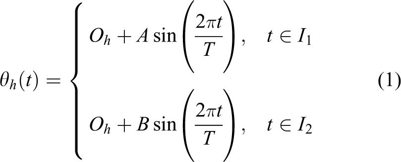
where O_h, O_k, A, B, C, t₂, and T are constants. Therefore, the problem of finding a stable biped locomotion at first is reduced to determining these seven constants. This may be done using an optimization algorithm. The joint trajectories resulting from these equations resemble the ones obtained from human locomotion data, as shown in the study by Shafii et al.⁸

The model may be extended to include arms movement by adding the shoulder-pitch joint. The equation we used to describe the trajectory of the left shoulder was

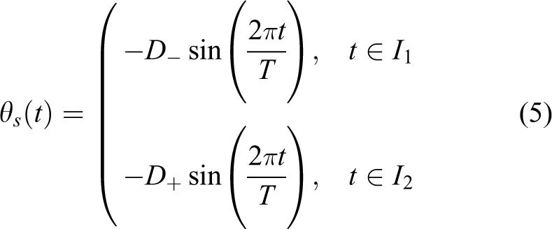
θ_{s} (t) = (\begin{matrix} - D_{-} sin (\frac{2 π t}{T}), & t \in I_{1} \\ - D_{+} sin (\frac{2 π t}{T}), & t \in I_{2} \end{matrix}

where D₋ and D₊ are new constants. Again, it is assumed that the right shoulder follows the same trajectory of the left one, except for a phase difference of π. Note that the shoulder joint is in phase opposition related to the leg joints of the same side, as a human does. In this case, we need to find nine constants.

A further extension may introduce joint movement in coronal plane (lateral direction) with the objective of trying to help the robot to take its foot off the ground. This idea is illustrated in Figure 2, and equation (6) is used to move the hip-roll joint. Differently from Shafii et al.,⁸ we maintain the torso allows upright. Note that our coronal movement pattern is qualitatively similar to the lateral torso sway that naturally arises in pendulum-based walking.¹ This kind of lateral torso sway motion helps maintaining the ZMP inside the support polygon during single support.²

Figure 2.

Proposed sequence of movements in coronal plane.

θ_{l} (t) = {\begin{array}{l} E sin (\frac{2 π t}{T}), & t \in I_{1} \\ 0, & t \in I_{2} \end{array}

where E is a new constant. Using this last model, we need to find 10 constants.

Three walking models were implemented herein following the ideas presented above. We call them

Simple model (SM): walking model that uses only the pitch joints of the legs.

Model with arms movement (AM): add arms movement to the simple model.

Complex model (CM): complete model considering movements from AM plus legs movement in coronal plane.

Note that our robot hardware has the required DOFs to implement all three walking models.

Optimization algorithms

To reduce the search space and make the optimization algorithms more efficient, it is convenient to limit the domains of optimization variables. In our specific problem, we are not interested in testing walking parameters and we certainly know that will make the robot fall. Accordingly, some tests were done to establish limits to the walking parameters, as shown in Table 1.

Table 1.

Limits for the domains of the walking models parameters.

Constant	Minimum	Maximum
O_h	−1.5	0
A	0.01	1.0
B	0.01	1.0
O_k	0	2.0
C	0	1.0
τ = t₂/T	0.1	0.9
T	0.1	0.7
D ₊	0	0.6
D ₋	0	0.6
E	0	0.5

We considered two approaches for walk optimization: one is based on particle swarm optimization (PSO) and the other one is based on genetic algorithms (GAs). For further details about the fundamentals of these approaches, please refer, respectively, to the studies by Shi and Eberhart¹¹ and Holland.¹²

PSO setup

The natural choice is to consider that each particle is in a D-dimensional space, where D is the number of constants to be determined. The search space is given by the limits shown in Table 1. The performance function is task-dependent and is presented in “Simulation setup for experimental analysis” section.

In the basic implementation of PSO, particles can reach high unrealistic speeds and get out of the search space boundaries. To avoid these problems, we made modifications to the basic PSO algorithm. First, we update a particle velocity using the following usual rule¹¹

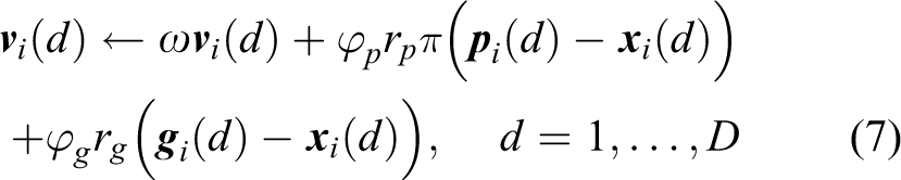
v_{i} (d) \leftarrow ω v_{i} (d) + ϕ_{p} r_{p} π (p_{i} (d) - x_{i} (d)) + ϕ_{g} r_{g} (g_{i} (d) - x_{i} (d)), d = 1, \dots, D

where D is the dimension of the search space; ω, ϕ_p, and ϕ_g are PSO parameters usually called inertia weight, cognitive parameter, and social parameter, respectively; r_p and r_g are random numbers distributed uniformly in [0, 1]; and x _i and v _i are the position and the velocity of particle i, respectively. Then, after updating a particle velocity, we saturate its velocity by applying equation (8)

v_{i} (d) \leftarrow min (u (d) - l (d), max (l (d) - u (d), v_{i} (d))), d = 1, \dots, D

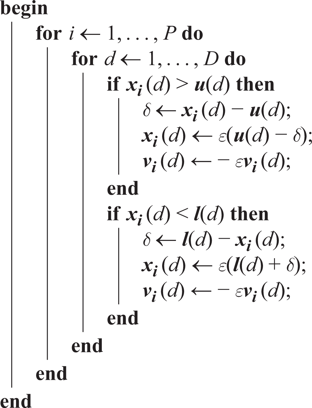
where u and l are the upper and lower bounds of the search space, respectively. The second modification keeps the particles inside the search space boundaries. We consider that when the particles cross search boundaries, an “inelastic collision” happens. With this mechanical inspiration, we developed a subroutine that is executed after we apply the velocity saturation through equation (8). The pseudocode for this subroutine is presented in algorithm 1, where P is the number of particles. Note that it introduces a new parameter ε, which we named “restitution coefficient,” following a mechanic analogy.

Finally, Table 2 presents the values used to configure the PSO.

Table 2.

Parameters values used for PSO.

Parameter	Value
Number of particles (P)	20
Inertia weight (ω)	0.9
Cognitive parameter (φ_p)	0.6
Social parameter (φ_g)	0.8
Restitution coefficient (ε)	0.7

PSO: particle swarm optimization.

Algorithm 1

Subroutine that simulates collisions of the particles against search space boundaries.

GA setup

To allow us to use GA, the operations of this algorithm were implemented as follows:

Chromosome: an array containing the D walking parameters. Each gene is a real number representing a parameter.

Fitness function: we used the equation shown in “Simulation setup for experimental analysis” section. Since this equation can yield a negative number, we just normalized every chromosome fitness by adding the smallest score of the current generation.

Mutation: with probability p_m for each gene, substitute the gene by a real value inside the respective limits presented in Table 1.

Selection: a standard roulette wheel selection was used.

Crossover: a standard one-point crossover mechanism was used.

Survival of the fittest: only the S_m fittest chromosomes are passed to the next generation, where S_m is the maximum allowed population size.

Finally, to configure GA, we used the parameter values presented in Table 3.

Table 3.

Parameters values for GA.

Parameter	Value
Initial number of individuals (S_i)	20
Maximum population size (S_m)	20
Number of individuals selected for reproduction (R)	10
Mutation probability (p_m)	0.05

GA: genetic algorithm.

Experimental setup

The USARSim simulator

USARSim is a high-fidelity robot simulator.¹³ Its current version is based on the Unreal Development Kit from Epic Games.¹⁴ Unreal uses NVIDIA PhysX¹⁵ as its physics engine, which is able model mechanics interactions (collision, friction, etc.) with high accuracy. Therefore, humanoid robots with high DOFs may be modeled using USARSim, as shown in the study by van Noort and Visser,¹⁶ with the Aldebaran Nao robot.¹⁷

The simulator comes with many robots, sensors and actuators, and model off-the-shelf. Implementation of new models is done using the tools provided by UDK. The most relevant tools used in this work were the UDK Editor—a 3-D model edition tool—and UnrealScrip—a proprietary high-level programming language.

Implementing the Robonova-I model

To implement a new robot model inside USARSim, the following basic steps are needed:

Develop CAD models of the robot;

Generate physical models based on the CAD models;

Program the robot model using UnrealScript;

Define extra parts, as sensors and actuators.

The implementation of the Robonova-I followed these steps, as explained in the next subsections.

Robonova-I simulation model

The CAD models used in this work were developed in a previous work using AutoCAD software from Autodesk, based on measurements taken on the real robot.¹⁸ Next, the pieces were imported in Autodesk 3D Studio Max, where graphic materials with simple colors patterns were assigned matching the real robot colors. Then, the models were exported to FBX format.

FBX files were imported in UDK Editor, where the 26-DOF simplified collision algorithm was used to generate physical models based on the CAD ones. After configuring each piece, the set was exported as a UPK (Unreal Package).

The next step involved creating an UnrealScript class to represent the robot, which was done based on an implementation made for the Aldebaran Nao robot.¹⁶ Each joints was implemented as a RevoluteJoint (a physical entity that connects two rigid bodies, allowing them to rotate with respect to each other around an axis), and collision between adjacent parts was disabled to avoid collision problems.

Finally, some sensors were added. Also, a USARSim special sensor called GroundTruth was attached to the torso of the robot. This sensor provides noiseless global position and orientation. Despite hard to obtain in the real world, these informations are very convenient for the learning process.

Figure 3 shows Robonova-I inside USARSim: physical models are presented as pink wireframe lines. On the left upper corner, there is a visualization of a camera attached to the robot head.

Figure 3.

Simulated Robonova-I inside USARSim.

Simulation setup for experimental analysis

To evaluate the robotic walking, we developed an experimental setup inside USARSim. The idea was to run experiments where the robot could walk for some time and a metric would be used to evaluate the observed walk performance.

The map “ExampleMap” (shown in Figure 4) was chosen for this experimental setup, as it provides a large area with flat ground and without obstacles. Considering the orientation that the robot is initialized inside this map, the X-coordinate axis points forward and the Y-axis to the right. Then, each experiment consisted of the following process:

Figure 4.

ExampleMap.

Start the simulated Robonova-I in a known position;

Wait 1.5 s so the robot can get in position for walking (e.g. bending its knees);

Let it walk for 20 s. The experiment is stopped if the robot falls;

Assess the walking performance using the following equation

D = (x - x_{o}) - | y - y_{o} | + 0.1 \times Δ t - \sum P_{i}

where (x₀, y₀) and (x, y) are initial and final positions of the robot, respectively. Δ_t is the time interval (in seconds) that the robot managed to move without falling, and ∑P_i represents the sum of possible punishments (shown in Table 4). The idea of using punishments is to notify the optimization algorithm that an undesirable event occurred.

Table 4.

Punishment values.

Punishment	Meaning	Value
P₁	Fall	50
P₂	Initial position unstable	80
P₃	Robot stayed in place	60

After some experimentation, we noted two problems:

The robot was frequently falling down when trying to make the first step, even with walks that were very stable when the walking was in steady state.

Due to the fact that walking is a very noisy process, it was often happening that a walking parameter set was misevaluated. The worst case was when a very fast but unstable walk made the robot upright for 20 s, thus receiving a very good evaluation. This was especially bad for PSO, because this algorithm is strongly guided by the best global solution.

To minimize these problems, two heuristics were implemented:

Instead of beginning the movement with nominal amplitudes, the robot linearly increases all amplitudes from zero to the nominal values during the first steps (after experimentation, we decided that this should be done during the first three steps).

Instead of using one experiment run to evaluate a walking parameters set, we decided to take an average of three experiment runs.

Optimization results

Table 5 shows the results from the optimization experiments, once the heuristics aforementioned were adopted. Each line in Table 5 refers to a single optimization instance. The following qualitative conclusions can be drawn from the results:

Table 5.

Experiments results.

Optimization algorithm	Walking model	Walk performance	Number of evaluations
GA	SM	6.16	1500
GA	AM	8.3	1500
GA	CM	5.77	1500
PSO	SM	5.58	860
PSO	AM	7.2	1449
PSO	CM	7.99	1493

GA: genetic algorithm; PSO: particle swarm optimization; SM: simple model; AM: arms movement; CM: complex model.

Adding arms movement improves the walking quality (if walking parameters are correctly adjusted).

Adding movement in coronal plane improves even more the walking quality (again, if walking parameters are correctly adjusted).

Adding more parameters makes optimization convergence harder, as expected.

Figures 5 and 6 show how the performance of the best individual in the population evolves with the number of evaluations for different executions of the optimization algorithms considered. SM, AM, and CM are the walking models defined in “Humanoid locomotion based on periodic functions” section. Table 6 shows the best walking parameters for each optimization case.

Figure 5.

Performance evolution (best individual) against number of evaluations for optimizations using GA. (a) Simple model. (b) Model with arms movement. (c) Complex model. GA: genetic algorithm.

Figure 6.

Performance evolution (best individual) against number of evaluations for optimizations using PSO. (a) Simple model. (b) Model with arms movement. (c) Complex model. PSO: particle swarm optimization.

Table 6.

Best walking parameters for each optimization case.

Constant	SM + GA	AM + GA	CM + GA	SM + PSO	AM + PSO	CM + PSO
O_h	−0.69	−1.2	−0.96	−0.64	−0.66	−0.87
A	0.23	0.33	0.37	0.27	0.5	0.51
B	0.43	0.37	0.68	0.35	0.56	0.7
O_k	0.98	1.6	0.99	0.85	0.83	1.23
C	0.4	0.51	0.76	0.3	0.6	0.46
τ = t₂/T	0.38	0.25	0.22	0.39	0.38	0.34
T	0.1	0.4	0.44	0.44	0.39	0.38
D ₊	—	0.58	0.58	—	0.17	0.54
D ₋	—	0.14	0.55	—	0.57	0.39
E	—	—	0.04	—	—	0.05

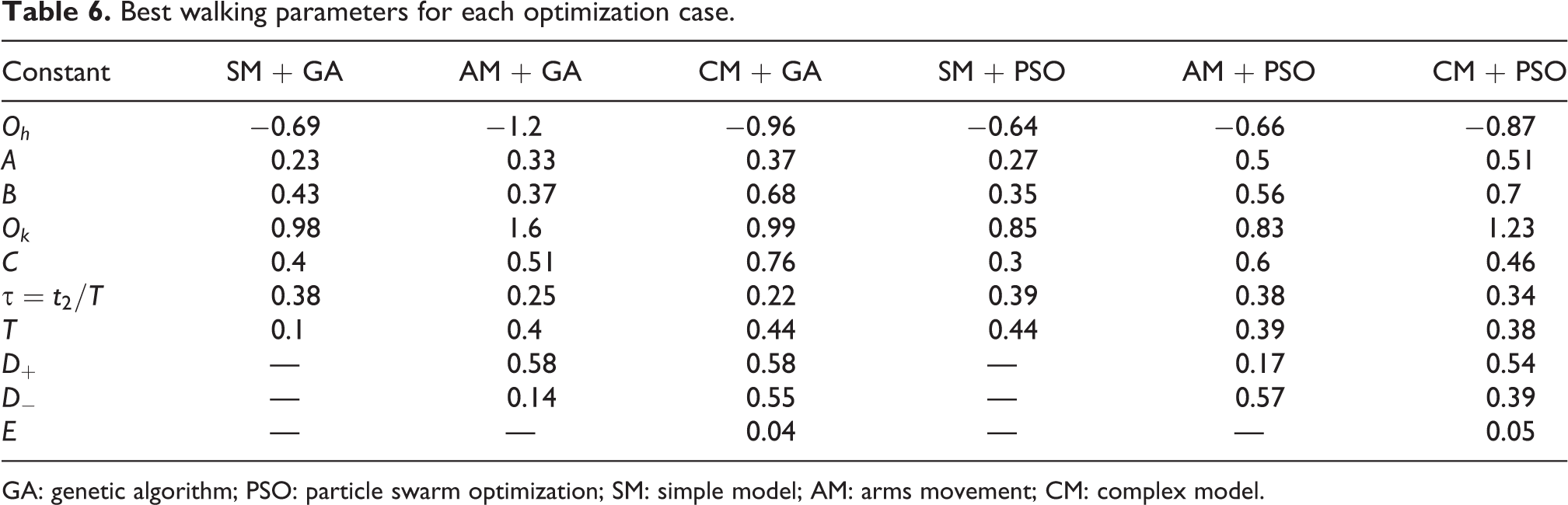
GA: genetic algorithm; PSO: particle swarm optimization; SM: simple model; AM: arms movement; CM: complex model.

Transferring to other domains

Transferring to a real robot

There are several factors that do not contribute to match simulation to a real robot setting, namely:

Physical models are approximations of CAD models.

Despite originating from the same model, real same type servomotors have small differences in torque and speed.

In the real robot, there are many mechanical phenomena that are usually not modeled in simulation due to computational complexity constraints: servomotor backlash, structural flexibility, and so forth.

In fact, humanoid locomotion is a complex problem and model imperfection may lead to very different walking behaviors. We thus expect that the parameters learned in simulation do not perform so well in the real robot.

To measure the walking speed in the real robot, we prepared the experiment setup shown in Figure 7. Ten experiments were ran for each walking, and we let the robot walk for 5 s and then measured the forward distance it moved.

Figure 7.

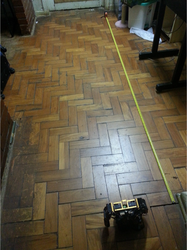
Experiment setup to measure the real robot speed.

As a first solution, we considered the simple model with parameters optimized in simulation. A walking pattern did occur, but the performance was poor, with the robot frequently falling and the trajectory making a turn to the right. After manually tweaking the walking period, we arrived at a stable walking despite a trajectory still with side turn. We noted that the robot was slipping because the movement amplitude was very high, so the foot movement was probably exceeding the maximum static friction provided by the floor. We then reduced the movement amplitudes until arriving at 60% of the original values. The walking obtained in this way had a forward speed of approximately 18.1 cm/s.

Then, we added arms movement and the forward speed improved to 21.5 cm/s. Moreover, the trajectory of the robot became more straight. Table 7 shows the obtained speeds for different walking models. We also show the original walks from the robot manufacturer (Hitec) and an improved version available at Hitec Robotics.¹⁹ Note that the final walking we developed outperforms all other tested. Figure 8 also shows a sequence of images to illustrate the real robot executing the walking with arms movement.

Table 7.

Comparison among different Robonova-I walks.

Walking	Mean speed (cm/s)	Standard deviation of speed (cm/s)	Number of falls (10 tests)
SM	18.08	1.05	0
AM	21.49	0.9	0
Forward walk¹	2.7	0.25	0
Fast walk¹	6.35	3.12	5
New fast walk²	19.2	1.3	0

SM: simple model; AM: arms movement.

Figure 8.

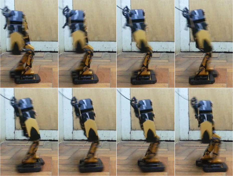
Image sequence showing the final walk on the real Robonova-I. The frame rate is 30 fps.

Transferring to a 3D soccer simulation domain

To provide further validation, we also implemented the walks in the RoboCup 3D Soccer Simulation League domain.²⁰ In this domain, twenty-two robots (11 in each team) play soccer in a simulation environment. The robotics simulator used is SimSpark,²¹ which uses open dynamics engine²² as its physics engine. The robot simulation model was inspired on the Aldebaran Nao robot.²³ To reduce our development effort, we used the base code magma-AF.²⁴

We executed the optimization process only for the simple and complex models using PSO, configured with the parameters presented in Table 8 and the search space limits shown in Table 9. The experiment setup used to evaluate the walking performance was very similar to the one we used in USARSim. The parameters learnt in this domain are shown in Table 10.

Table 8.

Parameters used to configure PSO for the 3D Soccer domain.

Parameter	Value
P	200
ω	0.7
ϕ_p	1.5
ϕ_g	1.5
ε	0.8

PSO: particle swarm optimization.

Table 9.

Search space limits for the 3D Soccer domain.

Constant	Minimum	Maximum
O_c	−1.0	0
A	0.01	1.0
B	0.01	1.0
O_j	0	1.5
C	0	1.5
τ = t₂/T	0.1	0.9
T	0.1	2.0
D ₊	0	1
D ₋	0	1
E	0	0.5

Table 10.

Best walking parameters learnt in the 3D Soccer domain using PSO.

Model	O_h	A	B	O_k	C	τ	T	D ₊	D ₋	E
SM	−0.032	0.13	0.55	0.60	0.91	0.35	0.14	—	—	—
CM	−0.10	0.11	0.57	0.66	0.97	0.35	0.18	0.19	0.24	0.06

PSO: particle swarm optimization.

To evaluate the performance of the learned walk, we compared it with the walk provided by the magma-AF base team. Fifty simulated experiments were performed for each walk model, where the robot was allowed to walk for 20 s. The experiment is interrupted if a fall is detected. Figure 9 shows an X-Y view of the 50 trajectories executed by the robot’s torso for each walk model. These trajectories show that the walks developed in this work far exceed the magma’s walk. Furthermore, the complex walk deviates much less than the simple one. In fact, the results show that the simple walk learnt is biased to the left, while we do not see a clear bias in the complex walk learnt.

Figure 9.

X–Y view of the 50 trajectories executed by the robot’s torso for each walk model.

Moreover, Table 11 shows some statistics regarding the results. “X distance” and “Y deviation” refer to the distance the robot has covered in the direction it is initially pointing and the distance it has deviated in the perpendicular direction at the end of the 20 s(or when it falls), respectively. Since the experiment is stopped when the robot falls, the experiment time gives a measure of the robot stability. These results are consistent with the trajectories shown in Figure 9. The best walk learnt covers about 355% more distance than the base team’s walk. Additionally, the gain in X distance was small (about 10%) by activating arms and coronal plane movements when compared with the simple walk learnt; however, the reduction in Y deviation (more than 40%) clearly shows that adding these features yields a better walking performance.

Table 11.

Results of the experiments done to evaluate the walks learnt in 3D Soccer domain.^a

	X-distance (m)		Y-deviation (m)		Experiment time (s)
Walk	Mean	Standard deviation	Mean	Standard deviation	Mean	Standard deviation	Number of falls (50 tests)
Simple model	11.86	2.52	3.77	2.86	19.67	2.41	1
Complex model	13.08	1.81	2.18	1.67	19.70	2.26	1
magma-AF	2.87	2.52	1.19	1.31	12.06	8.52	26

^aFifty experiments were executed for each walk model. In each experiment, the robot was allowed to walk during 20 s.

Figure 10 presents an image sequence showing the CM walk learnt in the 3D Soccer domain. To provide a better understanding between the effects of the arms and coronal movements on the learnt joint trajectories, Figure 11 shows the joint trajectories for the walks learnt in the 3D Soccer domain. Observe that the trajectories learnt for the leg joints legs are very similar between simple and complex models in this case.

Figure 10.

Image sequence showing the complex walk learnt in the 3D Soccer domain.

Figure 11.

Joint trajectories of the walks learnt in the 3D Soccer domain.

Conclusions

In this work, stable and fast walks for the Hitec Robonova-I robot were developed and presented. The approach used considered parameterized walking models, with TFS used to generate angular trajectories for joints. Adequate parameter values were determined using optimization algorithms, namely, GA and PSO.

Since optimizing directly on the real robot would probably result in hardware damage, we decided to follow an approach where a walk was learned in simulation and then adapted to the real robot. After manually tweaking the walk learned in simulation, we arrived at a walking that outperforms the original Robonova-I walking in the real robot. To provide further validation of the approach used, we executed the same process in the RoboCup 3D Soccer Simulation domain, where a simulated robot was also able to learn a fast and stable walk.

The approach presented here may be extended in future work. The model used allows only forward walking, but it is often convenient to be able to walk sideways and to change the direction the robot is facing. Other interesting research direction is to improve the walking model by adding more features. Also, the resulting gait is a pattern that is played over time without taking into account the robot state. Even using this open loop pattern, the real robot was able to walk stably and accommodate some perturbation and model error. However, the use of sensory feedback is expected to greatly improve the walk robustness. We are currently working on these improvements.

Footnotes

Author Note

Author Carlos H. C. Ribeiro is now affiliated to Aeronautics Institute of Technology, São José dos Campos, São Paulo, Brazil.

Declaration of conflicting interests

The author(s) declared no potential conflicts of interest with respect to the research, authorship, and/or publication of this article.

Funding

The author(s) received no financial support for the research, authorship, and/or publication of this article.

References

Kajita

Kanehiro

Kaneko

. The 3D linear inverted pendulum mode: a simple modeling for a biped walking pattern generator. In: Proceedings of the 2001 IEEE/RSJ international conference on intelligent robots and systems, Maui, Hawaii, USA, 29 October–3 November 2001, pp. 239–246.

Takenaka

Matsumoto

Yoshiike

. Real time motion generation and control for biped robot -1st report: walking gait pattern generation. In: Proceedings of the 2009 IEEE/RSJ international conference on intelligent robots and systems, St. Louis, USA, 11–15 October 2009.

Collins

Ruina

Tedrake

. Efficient bipedal robots based on passive-dynamic walkers. Science 2005; 307(5712): 1082–1085.

Hackenberger

. Balancing central pattern generator based humanoid robot gait using reinforcement learning. Master’s Thesis, Theoretical Computer Science, 2007.

Mochon

McMahon

. Ballistic walking. Journal of Biomechanics 1980; 13(1): 49–57.

Shafii

Khorsandian

Abdolmaleki

. An optimized gait generator based on Fourier series toward fast and robust biped locomotion involving arms swing. In: Proceedings of the IEEE international conference on automation and logistics, 2009.

Shafii

Aslani

Nezami

. Evolution of biped walking using truncated Fourier series and particle swarm optimization. In: Baltes

Lagoudakis

Naruse

Ghidary

(eds) RoboCup 2009, Atlanta, USA, 2010, pp. 344–354.

Shafii

Reis

Lau

. Biped walking using coronal and sagittal movements based on truncated Fourier series. In: RoboCup 2010: robot soccer World Cup XIV, lecture notes in computer science, 2010, pp. 324–335.

Hitec Robotics. Robonova-I English Instruction Manual.

10.

Yang

Chew

Zielinska

. A uniform biped gait generator with offline optimization and online adjustable parameters. In: Proceedings of the 2006 IEEE/RSJ international conference on intelligent robots and systems, 2006, pp. 4435–4440.

11.

Shi

Eberhart

. A modified particle swarm optimizer. In: The 1998 evolutionary computation proceedings, 1999.

12.

Holland

. Adaptation in natural and artificial systems. Michigan: The University of Michigan Press, 1975.

13.

Sycara

Nourkbaksh

Lewis

. Unified system for automation and robot simulation. http://sourceforge.net/projects/usarsim/, 2012. (accessed 4 November 2012).

14.

Epic Games. Unreal development kit. http://www.unrealengine.com/udk/, 2008–2012. (accessed 25 October 2012).

15.

Nvidia. Physx. http://www.geforce.com/hardware/technology/physx, 2012. (accessed 28 October 2012).

16.

van Noort

Visser

. Validation of the dynamics of a humanoid robot in USARSim. In: Proceedings of the performance metrics for intelligent systems workshop (PerMIS’12), March 2012.

17.

Albebaran Robotics. Nao H25: Humanoid Robot Platform. http://www.aldebaran-robotics.com/en/Discover-NAO/nao-datasheet-h25.html, 2012. (accessed 25 October 2012).

18.

Colombini

da Silva Simões

Martins

. A framework for learning in humanoid simulated robots. In: RoboCup 2007: Robot Soccer World Cup XI, 2008, pp. 345–352.

19.

Hitec Robotics. New source code with fast walk and fast turn. http://www.robonova.de/store/support/index.php?_m=downloads_a=viewdownloaddownloaditemid=93nav=0,5,7, 2006. (accessed 25 October 2012).

20.

RoboCup Federation. RoboCup. http://www.robocup.org/, 2012. (accessed 25 October 2012).

21.

Obst

Rollmann

. SPARK - a generic simulator for physical multiagent simulations. Computer Systems Science and Engineering 2005; 20: 347–356.

22.

Smith

. Open dynamics engine. http://www.ode.org/, 2012. (accessed 25 October 2012).

23.

SimSpark. SimSpark agents. http://simspark.sourceforge.net/wiki/index.php/Agents, 2012. (accessed 25 October 2012).

24.

Dorer

Glaser

Schindler

. http://robocup.hs-offenburg.de/uploads/media/magma3D-2011Release.tar.gz, 2011. (accessed 7 October 2014).

Stable and fast model-free walk with arms movement for humanoid robots

Abstract

Keywords

Introduction

Computational walk model for a biped robot

The biped robot model

Humanoid locomotion based on periodic functions

Optimization algorithms

PSO setup

GA setup

Experimental setup

The USARSim simulator

Implementing the Robonova-I model

Robonova-I simulation model

Simulation setup for experimental analysis

Optimization results

Transferring to other domains

Transferring to a real robot

Transferring to a 3D soccer simulation domain

Conclusions

Footnotes

Author Note

Declaration of conflicting interests

Funding

References