Acquisition of a space representation by a naive agent from sensorimotor invariance and proprioceptive compensation

Abstract

In this article, we present a simple agent which learns an internal representation of space without a priori knowledge of its environment, body, or sensors. The learned environment is seen as an internal space representation. This representation is isomorphic to the group of transformations applied to the environment. The model solves certain theoretical and practical issues encountered in previous work in sensorimotor contingency theory. Considering the mathematical description of the internal representation, analysis of its properties and simulations, we prove that this internal representation is equivalent to knowledge of space.

Introduction

Sensorimotor theory

Sensorimotor contingency theory argues that the acquisition of space knowledge in the brain is a result of the interaction between perception and body movement. “Passive perception” alone is not sufficient to create a representation of space, instead many authors propose “active percetion” in which action is a necessary component of perception. ^1,2 The connections between sensory inputs and motor outputs are defined by a general set of rules whose properties depend on the characteristics of the surrounding space. ^{2 –8} The agent is able to use its body to compensate for sensory changes. In response to sensory changes, which are a result of changes in the environment or body movements, the agent will move to counter the effect of the initial changes. Poincaré ^4,5 described the compensation algorithm as the capability of the body to compensate for a transformation of the environment. Nicod ^6,9 applied the concept of compensation to auditory signals and stated that a space representation can emerge when body movements are used in interaction with the auditory system. More recently, O’Regan and Noë ² used psychological arguments obtained from experiments on humans and animals to clearly define the sensorimotor contingency approach and outline its expectations. Philipona et al. ^7,8 performed physical simulations, modeling, and analyses of the tangent spaces of the manifold of sensorimotor interactions. These studies showed that it is possible to retrieve the dimension of the learned space for any sensory and motor dimensions. The algorithm of Philipona retrieved the dimension of the group of transformations in which their agent moved without any prior knowledge of it and without knowledge of the sensory and motor dimensions. Laflaquiere et al. ^10,11 implemented this type of algorithm in order to retrieve the dimensionality of the environment in which a robot moved its arm.

In a psychological study, Aytekin et al. ¹² demonstrated that humans use a sensorimotor approach to learn space from auditory stimulation. The group properties and the metric of the auditory space were shown to be captured by the human brain, thanks to sensorimotor interactions. Terekhov and O’Regan ^13,14 showed that an agent using internal compensation movements could acquire external movements and the metric without knowledge of the environment.

The present article extends the field of sensorimotor research by demonstrating a naive agent that learns the group properties of space and provides new insights into theoretical results. The naive agent creates a usable representation of space and retrieves its fundamental properties such as its group operation. The term “naive” indicates that before learning the agent had no awareness of space or its properties. Using compensation, this agent is able to learn an internal representation of space. We extend the Laflaquière and Terekhov models, merging their algorithms. Our results remove all ambiguity in the mathematical representation of space and extend the usability of the representation. This representation is itself a group and is isomorphic to the group of compensable transformations. The agent measures sensory signals from the environment, which correspond to changes in its perception. The change in perception can be due to movements generated by the agent (internal movement, external movement, or both), a change in the environment (a transformation applied to the sources of signal), or to a combination of these. The agent will act to compensate for these changes in order to retrieve the same signal it was experiencing before the change.

In this article, the agent’s proprioceptive capabilities alone are used to create a full representation of its environment without any a priori knowledge of it. This representation has the same properties as its embedding space (R²). The learning algorithm is based on the notion of compensation defined by Poincaré (Poincaré, 1898, 1902) for the visual perception of space.

In order to prove that our agent has learned a representation of space, we use the following points:

The agent captures invariant proprioceptive domains in a stationary environment, which provide an internal calibration for its own movements.

The agent learns the transformations of the environment by compensable movements (movements of the foot, retina, or both), which link environment transformation to body transformation.

The agent can distinguish between learned transformation and non-learned transformation (compensable and non-compensable).

The agent captures the properties of learned transformations.

The group properties for combinations of external movement are reproduced by the agent’s internal representation. When the agent uses its internal representation to predict or reproduce a combination of movements, the combinatory effect is preserved.

The internal representation is isomorphic to the group of transformations.

A handicapped agent that cannot apply the algorithm (no sensory matching) cannot learn the compensable movements and therefore cannot learn the space representation.

Using all of the above, we show that the internal representation is equivalent to a representation of space.

In the next section, we describe the agent in detail. We describe its sensory system and body. We explain the algorithm applied during learning and the theoretical requirements for proof that the agent learned a full representation of space. Next, we present the computational logic and calculations that have been applied to the agent. We present the solution used to validate our theoretical claims and discuss the effects studied. We then present our theoretical results and simulations. We compare the learned compensable transformations to noise and non-compensable transformations. We also show the proof of the group properties learned by the agent and its internal representation of space. Taking the example of an agent with a particular form of handicap, we show how this is reflected in terms of the representation of space. Finally, we discuss the results of the model and present future work.

Theoretical presentation

The environment

The environment is composed of a number of light sources. Signal propagation obeys physical laws and is generated by a simple ray tracing algorithm for each source. The environment and its state is defined by ∊. The different states of the environment are noted with the q subscript giving ∊_q to describe the environment in state q. All the possible states belong to the set $\epsilon :{∊}_q\in \epsilon$ .

The environment can be subject to transformation T and the environment will then be in a different state.

$T\left({∊}_q\right)={∊}_{q^{\prime }},T:\epsilon \to \epsilon$

1

The transformation of the environment ∊ can be rigid transformation (translation and rotation), geometrical transformation (scaling), or any type of transformation (noise, intensity change, and random movement of the sources of light). When subject to a rigid transformation, the effect applies on all the sources of signal with a displacement of their locations in the physical space.

Sensations of the change in the environment

The agent has a retina, which is sensitive to the source of lights. The retina is a detector composed of visual cells, which are sensitive to the sources depending on the source position relative to the sensor. Let s ∈ S describe the sensorial activity of the agent. The dimension of S is the dimension of the retinal signal given by the number of visual cells. An example of this type of sensory detector is shown in Figure 1 . The signals are measured by the agent’s detector. The detectors are sensitive to a signal emitted by the sources and the signal variation on a detector is directly linked to the source’s localization in the space surrounding the agent. The signals captured by the detector depend on location with a function

$s=\sigma (X^r,∊)$

2

Figure 1.

The signal measured by each visual cell depends on the distance between the sources i located at Xi and the retina located at X^r. The set of signals defines the visual signal vector, which depends on the number of cells in the retina. The signal is given by the function $\sigma \left(X^r,∊\right)={\displaystyle {\sum }_{i=0}^N}\sigma \left(X^i-X^r,∊\right)$ , where ∊ is the effect of the global position of the agent in the environment.

where X^r is the relative position of the retina in the agent and ∊ is the environment’s effect on the agent (which depends on the absolute position of the agent in the environment). The σ function is a binary relation between the environment and R^m where m is the dimension of the signal-measuring sensor $\sigma \left(X^r,∊\right)={\displaystyle {\sum }_{i=0}^N}\sigma \left(X^i-X^r,∊\right)$ where the X_i is the lights’ location in the environment relative to the retina. It is important to note that the signal function must be continuous and invertible.

Invertibility can be ensured by considering a sufficiently complex detector, that is, one composed of sufficient number of retina cells. We do not suppose we have a full domain where the function is invertible, however, in our simulation, we only got limitations with very few cells in the retina and this showed interesting defects in the space representation. Defects in the space representation obtained using an insufficient number of cells will be discussed later in the article. (The change in the environment can generate sensory variation in the agent.)

Agent description

The agent is a simple body composed of two moving parts: a foot which generates body displacements and a retina which can be moved inside the body (Figure 2). For simplicity, we present, in the Figure, a one-dimensional environment, however, our agent was validated and tested in a two-dimensional environment. The proprioceptive state of the agent p ( p ∈ Rⁿ) is defined by combining the retina proprioceptive state p ^r and the foot motor activity p ^f as $\mathit{p}=({\mathit{p}}^r,{\mathit{p}}^f{)}^{{\rm T}}\in \mathcal{P}={\mathcal{P}}_R\times {\mathcal{P}}_F$ . Where P_R and P_F are the sets of all proprioceptive values. The foot proprioceptive state ${\mathit{p}}^f\in {\mathcal{P}}_F$ can allow the agent to move both forward and backward.

Figure 2.

The agent is in a physical space and can move in any direction (left or right along X in this figure) by controlling a foot. The foot displacement is associated with the external proprioception p ^f . The agent has a retina which can move freely inside the body. The retina position depends on the internal proprioception p ^r . The environment is composed of a number of lights which can move together (not individually) in any direction.

In the following part of the article, we are using the subscripts q and q′ in order to distinguish the state of the studied objects. p _q and ${\mathit{p}}_{q\prime }$ are the proprioceptive states of the agent corresponding to two states q and q′. We are also using this notation to distinguish the states of the environment ∊_q and ${∊}_{q^{\prime }}$ . Using such a simple agent allows us to use precise mathematical tools to clarify the properties of space perception. Space and compensable transformations, as proposed by Poincaré, ³ are central to our study and are discussed in the two next sections.

The movements of the agent are of two kinds: internal when the agent moves its retina and external when the agent moves its foot. The effect of the movement of the retina is related to the proprioception of the retina p ^r and the relative position of the retina in the agent is given by a function Π

$X^r=\Pi \left({\mathit{p}}^r\right)$

3

The proprioception of the foot p ^f generates external movement. The body of the agent is fully displaced when the agent moves its foot. The movement of the foot is given by the function μ

$\Delta \text{Agent}=\mu ({\mathit{p}}^f)$

4

Applying the effect of μ( p ^f ) to the agent is equivalent to a geometrical transformation to its body location (rotation and translation). When the foot proprioceptive value p ^f is equal to 0, the agent is at rest.

Π and μ are bijective and thus are invertible functions. This bijectivity is a particular case that can be generalized. ¹⁵

The absolute position of the retina in the evironment can be given by the position of the agent in the environment and the relative position of the retina in the agent X^r. While the agent doesn’t know its absolute position, it can act by changing its retina position with the movements of its body. Only foot movements generate any displacement of the body. Foot movements are not bounded, while the retina movement is solely within the body of the agent. While this is a strong hypothesis, it is necessary for purely mathematical reasons. However, the limits of this hypothesis are not tested as we typically consider small movements centered on the agent’s body and only small foot movements are needed to compensate.

Compensable transformation

In 1895, H. Poincaré wrote his work on space and geometry. ³ He defined geometry in relation to a totally naive brain, which has access to its sensorimotor flow only. The geometry can be inferred by considering certain types of sensory changes. Of all the possible sensory variations, some occur without motor commands and, therefore, must be related to external changes. Some changes that are related to external rigid displacements can be compensated by the agent’s motor commands. In this case, the sensory variations due to the external changes and the motor commands are opposite, so that the initial and final sensory states are identical. This is what is meant by compensable. Because the function linking the positions of light sources and the agent sensor signal is invertible, for a stationary agent, we can state that for every change of the environment, the sensory perception of the agent also changes. When considering different positions of the agent in the environment with identical values of the proprioceptive state vector p (identical retina position and foot activity), the signals measured by the sensor are necessarily different. In the general case, the agent is unable to infer its sensorial variations from variations in its proprioceptive state. However, compensable transformations can be thought of as a type of sensorial variation due to external transformations that are compensated by a specific movement of the agent. These compensable transformations can be detected by the agent. According to Poincaré’s proposition, the set of compensable transformations is a group and is equivalent to the group characterizing the external geometric space. By experiencing the compensable transformations, the agent can capture the most important properties of the (Euclidean) space in which it moves.

Capturing the set of compensable transformations

In this section, we introduce the formalism for compensable transformations by defining Φ as a set of binary relations φ^T that will allow us to build a representation of the group of compensable transformations T. We consider two cases: auto-compensable transformations in a stationary environment and compensable transformations more generally. Making this distinction allows the set of φ^T to map specific transformations T unambiguously. Initially, the φ^T functions were proposed by Terekhov et al. ^13,14 They are built from a catalog of all compensable transformations the agent detects. By matching identical sensory inputs before a change and after compensation, φ^T functions map proprioception observed before a change to proprioception observed after the compensation.

For a given displacement T of the environment, the agent will recover the same function φ^T for both different initial positions and different environments. As shown by Terekhov and O’Regan, ¹⁴ the functions φ^T provide the agent with the notion of space.

(In this article, the φ^T are not functions but binary relation as they are not unique mappings from P to P. However they are real functions in the article of Terekhov.)

Compensable transformations

Let $\left(s,{\mathit{p}}_q\right)\in \mathcal{S}\times \mathcal{P}$ describe the state of the agent in the environment. After a given rigid displacement of the environment (lights moving in our case), the agent’s new state is $\left(s\prime ,{\mathit{p}}_q\right)$ . Such a transformation is compensable if there exists a new proprioceptive state ${\mathit{p}}_{q^{\prime }}$ corresponding to a displacement of the agent in the environment and the resulting state is $\left(s″,{\mathit{p}}_{q^{\prime }}\right)$ with s″ = s. In other words, the agent has moved in order to recover the initial perceptual state. Given a compensable transformation of the environment T, the function φ^T is the mapping between P and itself such that for all proprioceptive states p _q ∈ P, one has ${\mathit{p}}_{q^{\prime }}={\phi }_T\left({\mathit{p}}_q\right)$ , where ${\mathit{p}}_{q^{\prime }}$ is the new proprioceptive state which compensates for T

${\phi }_T:\mathcal{P}\to \mathcal{P},{\mathit{p}}_q\to {\mathit{p}}_{q^{\prime }}={\phi }_T\left({\mathit{p}}_q\right)$

5

This definition does not depend on the perceptual state s. This is a consequence of the definition of compensable transformations. Cases where s″ = s can be found as long as the agent can evaluate its sensory flow. Difficulties arise when discussing how an agent can detect such coincidences from the sensorimotor flow alone, without a priori knowledge. How can it infer for a set of $\left({\mathit{p}}_q,{\mathit{p}}_{q^{\prime }}\right)$ that they correspond to the same φ^T? That is, how does it determine that they compensate for the same unknown external compensable transformation T? Terekhov and O’Regan proposed a solution ¹⁴ whereby they collected all the agent compensations corresponding to the same external transformation T and repeated for all other values of T. However, as the agent itself does not have access to T, this solution is somewhat artificial. In this article we propose a new solution to this problem by introducing the notion of auto-compensable transformation. In this case, the environment is stationary. Since this is not known by the agent, we must also introduce the identity transformation of the agent’s body.

(As mentioned earlier, while the φ_T are functions in case of the Terekhov’s article, in our case there are not. However, when we keep the foot proprioceptive state constant before and after the compensation (respectively the retina proprioceptive value before and after the transformation of the environment), the compensation φ_T becomes a function as there is a unique retina state compensating the applied transformation (respectively for the foot). When the environment is stationary, φ₀ is a function (see next section).

In the article, we will then use the term of function even if it can be seen as an inaccurate term.

Auto-compensable transformation

An auto-compensable transformation is the displacement of a part of the agent’s body (e.g. retina), which compensates for sensorial variations induced by the movement of another part of the agent’s body (e.g. foot displacement). The distinction between auto-compensation and compensation more generally is that the transformation T is fully determined by the agent in the case of auto-compensation. The agent can then build a set of functions φ^T, which can be used as internal references to represent external compensable transformations. In order to avoid any confusion between the agent’s transformations T and external transformations, the environment must remain stationary when determining the function φ^T. However, the agent cannot know whether the environment is stationary or not. This problem has been discussed by Roschin and Frolov, ¹⁶ Laflaquière, ¹⁷ and more recently by Marcel et al. ¹⁵ without finding a fully satisfactory solution. We will address this by introducing the identity transformation. The identity transformation can be considered a simple saccadic movement. After a displacement of the agent’s foot, the sensorial state of the retina changes. The agent then recovers the initial proprioceptive state of the foot by performing the exact inverse displacement of the foot. The initial sensorial state of the retina will be recovered. If it is not, then the agent can state that the environment changed during the identity transformation. Therefore, by retaining only those transformations which do not involve movements of the external environment, the agent can build unambiguous φ^T functions.

Φ the set of sensorimotor functions

As previously defined, Φ is the set of functions φ^T, which maps the proprioceptive states onto themselves. We will show that our agent can capture the set of compensable transformations T and that it learns the group properties of this set. Using equation (5), we show (in Appendix 1) that if the agent’s state modification from p _q to ${\mathit{p}}_{q^{\prime }}$ compensates for the environment transformation T, we have

${\mathit{p}}_{q^{\prime }}={\phi }_T\left({\mathit{p}}_q\right)=\left(\begin{array}{c}\Pi \circ \mu \left({\mathit{p}}_q^f\right)\circ T\circ \mu {\left({\mathit{p}}_{q\prime }^f\right)}^{-1}\circ {\Pi }^{-1}\left({\mathit{p}}_q^r\right)\\ {\mathit{p}}_{q\prime }^f\end{array}\right)$

6

$\Pi \left(p_q^r\right)=X_q^r$ is the function that describes the sensor position relative to the agent’s body in the physical space given the agent’s proprioceptive state ${\mathit{p}}_q^r$ . $\mu \left({\mathit{p}}_q\right)$ is the function that describes the movement of the agent’s body given the foot proprioceptive state ${\mathit{p}}_q^f$ . We distinguish between the reverse function of μ, ${\mu }^{-1}\left(X_q\right)={\mathit{p}}_q^f$ , and the opposite function of μ, $\mu {\left({\mathit{p}}_q^f\right)}^{-1}$ , which is the opposite displacement of $\mu \left({\mathit{p}}_q^f\right)$ . The function Π⁻¹ is the inverse function of Π.

In this article, we present the φ^T functions and their properties and demonstrate that there is a calculable solution. It is important to note that the agent has no knowledge of Π and μ. Only the mapping of p _q to ${\mathit{p}}_{q^{\prime }}$ is known. We can describe this mapping by a mathematical function. In order to do so, we first consider transformations that are auto-compensable in a stationary environment before moving to the general case of a nonstationary environment.

Auto-compensable transformation

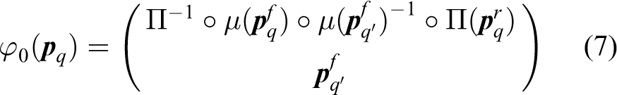
When considering the auto-compensable transformation, the environment is stationary. We calculate φ₀, where 0 indicates no movement of the environment. When the agent moves its foot, it compensates for the movement with its retina. The absolute position of the retina does not change. It is the same before the foot movement and after the compensating movement of the retina. After the foot movement, the environment perceived by the agent is changed in accordance with the physical laws of signal propagation and perception. Compensation is the act of retrieving the initial signal by a movement different to that which generated the difference. For every foot movement and initial retina position, the final retina position corresponding to the compensated movement is unique in a stationary environment (bijectivity of Π and μ). The signal measured after the compensating retina movement is compared to that before the foot movement. The algorithm applied to the agent is as follows

The agent is in an environment at a given location X_q, with the retina at a given position $X_q^r=\Pi \left({\mathit{p}}_q^r\right)$ . The agent can move its foot and generate a body displacement $\mu \left({\mathit{p}}_q^f\right)$ , where ${\mathit{p}}_q^f$ is the foot state.

The agent moves to a new location $X_{q^{\prime }}$ in response to a foot movement induced by the foot motor activity ${\mathit{p}}_{q\prime }^f$ . The transformation generating the displacement is given by $X_q\stackrel{\mu \left({\mathit{p}}_{q\prime }^f\right)}{\to }{X}_{q^{\prime }}$ .

The agent compensates for the foot movement by moving its retina in such a way that the retina visual perception is the same before and after the initial movement. The practical implementation is given in Appendix 1. What the agent sees after compensation is exactly what it saw before the foot movement. The final relative retina position is measured only by its internal state ${\mathit{p}}_{q\prime }^r$ .

The agent creates an internal representation of auto-compensation by mapping the initial internal state p _q to the final state ${\mathit{p}}_{q^{\prime }}$ , ${\phi }_0\left({\mathit{p}}_q\right)={\mathit{p}}_{q^{\prime }}$ .

We show in the Appendix 1 that

${\phi }_0\left({\mathit{p}}_q\right)=\left(\begin{array}{c}{\Pi }^{-1}\circ \mu \left({\mathit{p}}_q^f\right)\circ \mu {\left({\mathit{p}}_{q\prime }^f\right)}^{-1}\circ \Pi \left({\mathit{p}}_q^r\right)\\ {\mathit{p}}_{q\prime }^f\end{array}\right)$

7

Compensable transformation

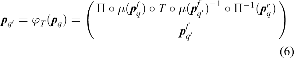
In this case, the environment is not stationary. When the environment is moved, the agent compensates by movement of the foot, retina, or both. The signal on the sensor is the same when measured before the movement of the environment and after the compensating movement of the agent. The algorithm is as follows

The agent is in an environment at a given location X_q, with the retina at a given position $X_q^r=\Pi \left({\mathit{p}}_q^r\right)$ . The agent can move its foot and generate a body displacement based on the function $\mu \left({\mathit{p}}_q^f\right)$ where ${\mathit{p}}_q^f$ is the foot state.

The environment is moved to ${∊}_{q^{\prime }}$ with ${∊}_q\stackrel{T}{\to }{∊}_{q^{\prime }}$ .

The agent compensates the external movement by either:

• A foot movement only. The body is moved in such a way that its retina visual perception is the same before and after the initial movement. The retina proprioceptive value remains unchanged. The foot proprioceptive value is ${\mathit{p}}_{q\prime }^f$ .

• A retina movement only. The body is not moved but the retina is moved in such a way that its retina visual perception is the same before and after the initial movement. The retina proprioceptive value is ${\mathit{p}}_{q\prime }^r$ . The final foot proprioceptive value is 0.

• Both foot and retina movement. Both the body and retina are moved in such a way that the retina visual perception is the same before and after the initial movement. The foot proprioceptive value is ${\mathit{p}}_{q\prime }^f$ . The retina proprioceptive value is ${\mathit{p}}_{q\prime }^r$ .

The agent creates an internal representation of the transformation T by mapping the initial internal state of the agent ${\mathit{p}}_q=\left(\begin{array}{c}{\mathit{p}}_q^r\\ {\mathit{p}}_q^f\end{array}\right)$ to the final state ${\mathit{p}}_{q^{\prime }}={\phi }_T\left({\mathit{p}}_q\right)=\left(\begin{array}{c}{\mathit{p}}_{q\prime }^r\\ {\mathit{p}}_{q\prime }^f\end{array}\right)$ .

We show in the Appendix 1 that

${\phi }_T({\mathit{p}}_q)={\phi }_T\left(\begin{array}{c}{\mathit{p}}_q^r\\ {\mathit{p}}_q^f\end{array}\right)=\left(\begin{array}{c}{\Pi }^{-1}\circ \mu ({\mathit{p}}_q^f)\circ T\circ \mu {({\mathit{p}}_{q\prime }^f)}^{-1}\circ \Pi ({\mathit{p}}_q^r)\\ {\mathit{p}}_{q\prime }^f\end{array}\right)$

8

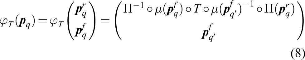
The set of φ_T( p ) defines a manifold in internal state space and can be used to show that the agent captures the geometrical space as defined by Poincaré. ³ The acquired knowledge is a space representation given that its properties mathematically correspond to those of space (including its group properties and the isomorphism with the compensable transformation set). This is discussed in the section “Φ is a representation of the geometrical space.” Figure 3 illustrates the steps of the coincidence algorithm outlined above.

Figure 3.

The matching coincidence algorithm is based on the comparison of the signal measured by each of the retina’s cells before an external movement is applied to the agent and after the compensating retina internal movement.

Φ is a representation of the geometrical space

As outlined previously, we will show that the set Φ of functions φ^T that corresponds to the mapping of proprioceptive states to compensable transformations has all the properties of the external space in which the agent is situated. The agent is capable of capturing the relevant properties even though it is not aware that such a set of transformations is a group. Thus, the set Φ of φ^T is a group and is also isomorphic to the set of T.

Combinatory property

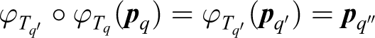
The combinatory operation ∘ on the set of φ^T functions is defined such that for any T_q, $T_{q^{\prime }}$ there exists $T_{q^{″}}$ such that ${\phi }_{T_{q^{\prime }}}\circ {\phi }_{T_q}={\phi }_{T_{q^{″}}}$ . In other words, the combination of two compensable transformations is itself a compensable transformation.

Demonstration: From the construction of the function φ^T, for any compensable transformation T, there is an associated function φ^T. Using the definition of a compensable transformation, there exists an action, which compensates for an external transformation. The compensation can be either an internal or external movement. As the displacement caused by the movement of the foot can be any length $(\mu \left({\mathit{p}}^f\right))$ , all combinations of compensable transformations can be compensated by foot movement. Thus, any combination of compensable transformations is compensable.

It is also the case that $\forall T_q,T_{q^{\prime }}$ and $T_{q″}$ where $T_{q^{\prime }}\circ T_q=T_{q″}$ then ${\phi }_{T_{q^{\prime }}}\circ {\phi }_{T_q}={\phi }_{T_{q″}}={\phi }_{T_{q^{\prime }}\circ T_q}$ .

Demonstration

We begin with

${\phi }_{T_q}\left({\mathit{p}}_q\right)={\mathit{p}}_{q^{\prime }}$

9

Applying equation (9) twice gives

${\phi }_{T_{q^{\prime }}}\circ {\phi }_{T_q}\left({\mathit{p}}_q\right)={\phi }_{T_{q^{\prime }}}\left({\mathit{p}}_{q^{\prime }}\right)={\mathit{p}}_{q″}$

Combining these functions with equation (8), we obtain

$\begin{array}{c}{\mathit{p}}_{q″}={\phi }_{T_{q^{\prime }}}\left({\mathit{p}}_{q^{\prime }}\right)=\left(\begin{array}{c}{\Pi }^{-1}\circ \mu \left({\mathit{p}}_{q″}^f\right)\circ T_{q^{\prime }}\circ \mu {\left({\mathit{p}}_{q\prime }^f\right)}^{-1}\circ \Pi \left({\mathit{p}}_{q\prime }^r\right)\\ {\mathit{p}}_{q″}^f\end{array}\right)\\ =\left(\begin{array}{c}{\Pi }^{-1}\circ \mu \left({\mathit{p}}_{q″}^f\right)\circ T_{q^{\prime }}\circ \mu {\left({\mathit{p}}_{q\prime }^f\right)}^{-1}\circ \Pi \circ {\Pi }^{-1}\circ \mu \left({\mathit{p}}_{q\prime }^f\right)\circ T_q\circ \mu {\left({\mathit{p}}_q^f\right)}^{-1}\circ \Pi \left({\mathit{p}}_q^r\right)\\ {\mathit{p}}_{q″}^f\end{array}\right)\\ =\left(\begin{array}{c}{\Pi }^{-1}\circ \mu \left({\mathit{p}}_{q″}^f\right)\circ T_{q^{\prime }}\circ T_q\circ \mu {\left({\mathit{p}}_q^f\right)}^{-1}\circ \Pi \left({\mathit{p}}_q^r\right)\\ {\mathit{p}}_{q″}^f\end{array}\right)\\ =\left(\begin{array}{c}{\Pi }^{-1}\circ \mu \left({\mathit{p}}_{q″}^f\right)\circ T_{q″}\circ \mu {\left({\mathit{p}}_q^f\right)}^{-1}\circ \Pi \left({\mathit{p}}_q^r\right)\\ {\mathit{p}}_{q″}^f\end{array}\right)\\ ={\phi }_{T_{q″}}\left({\mathit{p}}_q\right)={\phi }_{T_{q^{\prime }}\circ T_q}\left({\mathit{p}}_q\right)={\phi }_{T_{q^{\prime }}}\circ {\phi }_{T_q}\left({\mathit{p}}_q\right)\end{array}$

The combination of φ^T functions does not depend on the intermediary steps selected by the agent.

Group property

The axioms necessary to validate a group are closure, associativity, the existence of an identity, and the existence of an inverse for every element of the group.

• Closure

$\forall \mathit{p}\in \mathcal{P},\forall {\phi }_{T_q},{\phi }_{T_{q^{\prime }}}\text{then} {\phi }_{T_{q^{\prime }}}\circ {\phi }_{T_q}\left(p\right)\in \mathcal{P}$

10

where P is the set of possible proprioceptive measures of the retina and foot.

This first property is obvious. It comes from the learning algorithm where the agent changes its proprioceptive state with a retina or foot movement to compensate for an external agent movement. The result of applying ${\phi }_{T_q}$ to any $\mathit{p}=\left(\begin{array}{c}{\mathit{p}}^r\\ {\mathit{p}}^f\end{array}\right)$ belongs to P. We must demonstrate that $\forall \mathit{p}\in \mathcal{P},\forall T_q$ and $T_{q^{\prime }}$ then ${\phi }_{T_{q^{\prime }}}\circ {\phi }_{T_{q^{\prime }}}\left(\mathit{p}\right)\in \mathcal{P}$ .

Demonstration: From the algorithm, we have $\forall {\mathit{p}}_q\in \mathcal{P},\forall T_q$ then ${\phi }_{T_q}\left({\mathit{p}}_q\right)\in \mathcal{P}$ . As ${\phi }_{T_q}\left({\mathit{p}}_q\right)={\mathit{p}}_{q^{\prime }}$ , we apply the same logic: $\forall {\mathit{p}}_{q^{\prime }}\in \mathcal{P},\forall T_{q^{\prime }}$ then ${\phi }_{T_{q^{\prime }}}\left({\mathit{p}}_{q^{\prime }}\right)={\phi }_{T_{q^{\prime }}}\circ {\phi }_{T_q}\left(\mathit{p}\right)\in \mathcal{P}$

• Associativity

$\forall {\phi }_{T_q},{\phi }_{T_{q^{\prime }}},{\phi }_{T_{q″}}\text{then} {\phi }_{T_q}\circ \left({\phi }_{T_{q^{\prime }}}\circ {\phi }_{T_{q″}}\right)=\left({\phi }_{T_q}\circ {\phi }_{T_{q^{\prime }}}\right)\circ {\phi }_{T_{q″}}$

11

Demonstration

${\phi }_{T_q}\circ \left({\phi }_{T_{q^{\prime }}}\circ {\phi }_{T_{q″}}\right)={\phi }_{T_q}\circ {\phi }_{T_{q^{\prime }}\circ T_{q″}}={\phi }_{T_q\circ T_{q^{\prime }}\circ T_{q″}}={\phi }_{T_q\circ T_{q^{\prime }}}\circ {\phi }_{T_{q″}}=\left({\phi }_{T_q}\circ {\phi }_{T_{q^{\prime }}}\right)\circ {\phi }_{T_{q″}}$

• Identity

$\forall {\phi }_T,{\phi }_0\text{then}{\phi }_T\circ {\phi }_0={\phi }_0\circ {\phi }_T={\phi }_T$

12

where φ₀ is the identity

• Inverse

$\forall {\phi }_T\text{then}{\phi }_T\circ {\phi }_T^{-1}={\phi }_T^{-1}\circ {\phi }_T={\phi }_0$

13

Demonstration for both identity and inverse:

In the group of transformations, ∀T we have $T\circ T^{-1}=Id$ which implies $\forall T,T^{-1}\text{then}{\phi }_T\circ {\phi }_{T^{-1}}={\phi }_{T\circ °T^{-1}}={\phi }_0$ .

This implies that ${\phi }_T^{-1}={\phi }_{T^{-1}}$

which proves the existence of an identity element $\left({\phi }_0\right)$ and the existence of a inverse function ${\phi }_T^{-1}={\phi }_T^{-1}$ for any φ^T.

These points demonstrate that the set Φ of the functions φ^T is a group.

There is an isomorphism between the set of compensable transformations T and the set of functions φ^T

In order to prove there is an isomorphism, we have to prove that the two sets have the same dimension and that the φ^T is linear and injective.

For the dimension of both sets, we are using previous work from Philipona et al. ^7,8 and Laflaquiere et al., ¹¹ which show that the internal representation of a compensatory agent has the same dimension as the geometrical space of transformation.

For linearity, we have shown that $\forall T_q,T_{q^{\prime }}$ then ${\phi }_{T_q}\circ {\phi }_{T_q}={\phi }_{T_q\circ T_{q^{\prime }}}$ . In the limit of compensability, we can easily extend it to $\forall T_q,T_{q^{\prime }},\alpha ,\beta$ then ${\phi }_{\alpha T_q}\circ {\phi }_{\beta T_{q^{\prime }}}={\phi }_{\alpha T_q\circ \beta T_{q^{\prime }}}$ which is the expected linearity.

To show that the φ^T are injective, we must prove that $\forall T_q,T_{q^{\prime }}$ if ${\phi }_{T_q}={\phi }_{T_{q^{\prime }}}$ then $T_q=T_{q^{\prime }}$ . Since the set of φ^T is a group, for every item in the set, there is a reverse function. Thus, ${\phi }_{T_q}={\phi }_{T_{q^{\prime }}}$ then ${\phi }_{T_q}\circ {\phi }_{T_{q^{\prime }}}^{-1}=Id={\phi }_{T_q\circ T_q^{\prime }-1}$ . Previously, we determined that if ${\phi }_T=Id$ , then $T=Id$ . Therefore $T_q\circ T_{q^{\prime }}-=Id$ and $T_q=T_{q^{\prime }}$ .

Theses points demonstrate that the set of functions φ^T is isomorphic to the set of compensable transformations and is thus a space representation.

Computation

Learning phase: Algorithm for computation of φ^T

In this section, we present the algorithm used to calculate φ^T where T is the external transformations applied to the agent. The set of transformations is a set of translations in two dimensions.

For the simulation, we considered a limited set of transformations of the environment T and a limited set of possible compensations (both foot and retina; see Appendix 1 for details). Applying this algorithm allowed us to calculate the complete set of functions ${\phi }_T\left({\mathit{p}}_q\right)={\mathit{p}}_{q^{\prime }}$ .

Using φ^T functions to retrieve movement

By referencing the memorized tuples of three elements $\left(T,{\mathit{p}}_q,{\mathit{p}}_{q^{\prime }}\right)$ , the combination of any two can be used to retrieve the third. There are multiple possible solutions for ${\mathit{p}}_{q^{\prime }}=\left(\begin{array}{c}{\mathit{p}}_q^r\\ {\mathit{p}}_q^f\end{array}\right)$ given p _q and T.

φ^T functions are only sensitive to compensable transformations

In order to test the algorithm, we applied transformations other than those the agent learned. We first applied a continuous transformation, where the length of translation is not a multiple of the basic step size used in the computation. We then applied a scaling transformation, where the source objects are deformed by homothetic deformation. We also added random noise to the source light signals, with an amplitude ranging from 10% to 500% of the initial signal. Starting with a random initial retina proprioceptive state ${\mathit{p}}_q^r$ and a random foot movement ${\mathit{p}}_q^f$ , we applied a random transformation T and then compensated for it, giving the final retina proprioceptive state ${\mathit{p}}_{q\prime }^r$ and foot action proprioceptive state ${\mathit{p}}_{q\prime }^f$ . We then retrieved ${\phi }_{T_q}$ from the best proprioceptive set $\left({\mathit{p}}_q,{\mathit{p}}_{q^{\prime }}\right)$ and extracted the associated T_q. We compared the applied T_a and extracted T_e (note that the T_q found from the algorithm is noted as the extracted T_e. When applying unknown (or non-compensable) transformations, coincidence matching could not be done. That is, it was not possible to match the states before and after movement. Exact matching was not possible and the error on the comparison of sensory measures increased with the difference between the initial image and the final image. The error between the applied T_a and the extracted T_e also became more significant as we measured $\parallel T_a,T_e\parallel$ . This test was repeated for 1000 transformations, starting with random retina positions and we calculated the error between the applied movement and the compensated transformation for the best tuple $\left({\mathit{p}}_q,{\mathit{p}}_{q^{\prime }}\right)$ .

Internal space as a group of transformations

A calculation was performed for the full set of points in the combined φ^T in order to verify ${\phi }_{T_1}\circ {\phi }_{T_2}={\phi }_{T_3}$ then $T_3=T_1\circ T_2$ . For any random transformations T₁ and T₂, we calculated $T_3=T_1\circ T_2$ . We then compared ${\phi }_{T_3}$ acquired directly from the set of φ^T and the calculated ${\phi }_{T_1\circ T_2}={\phi }_{T_1}\circ {\phi }_{T_2}$ . As shown in the paragraph on the validation of the group axioms, this property proves the associativity, identity, and inverse axioms.

Testing parameters and mathematical functions

Our initial selection of functions and parameters did not affect our results. In order to demonstrate this, we repeated the simulations with multiple sets of proprioceptive functions $\left(\Pi \left({\mathit{p}}^r\right)=X^r\right)$ and varied the ratio of the applied movements to the retina or foot movements.

Figure 4 illustrates the simple and complex proprioceptive models used in this article.

Figure 4.

Comparison between simple and complex agents. (a) Simple agent. When the retina moves in the direction X, only the proprioceptive p_x is transformed into ${p^{\prime }}_x$ . p_y is not affected by the movement and (b) complex agent. When the retina moves in any direction, all proprioceptive detectors are affected $\left(p_1,p_2,\text{and}{p}_3\right)$ then $\left({p^{\prime }}_1,{p^{\prime }}_2,\text{and}{p^{\prime }}_3\right)$ .

In all simulations, we used a grid for the environment and a grid for the body displacement. The relevant values for the simulation are as follows:

The number of steps the agent moves on a grid within the environment, # Steps.

The ratio of environment displacement step size to body movement step size, $\frac{\Delta e}{\Delta b}$ .

The proprioceptive function measure $\Pi (p)$ , which is one of:

Affine function: $\Pi \left(p\right)=X=a\times p+b$

Logarithmic function: $\Pi (p)=X=\sqrt{\ln (1-p)}$

Proprioceptive coupling

Uncoupled proprioceptive function (simple model). Movement in any direction is associated with a single proprioceptive measure. $\Pi \left(p_x^r\right)=x$ and $\Pi \left(p_y^r\right)=y$ . This generates two independent φ^T functions, φ^T and φ^T, where $T(x,y)$ is the applied transformation.

Coupled proprioceptive function (complex model). Movement in any direction affects all proprioceptive measures. $\Pi \left(p\right)=\Pi \left(p_1^r,p_2^r\mathrm{,},p_i^r\mathrm{,},p_n^r\right)=\left(x,y\right)$ . This generates a single multidimensional φ^T, where T is the applied transformation.

The retina of the agent is composed of randomly located cells in the retina. In the next section, we present the results of varying sensory parameters such as the number of cells and retina size in the simulations.

Results

Compensable movement versus non-compensable movement

The estimated displacement when applying either compensable movement or non-compensable movement is listed in Table 2. Since we know the applied transformation (even though the agent does not), we know the expected position after the transformation. We compare this to the agent’s estimated position after transformation and calculate the difference between them. When the difference is zero, the expected and estimated positions are identical. For this test, we selected 1000 random movements (for each type of transformation) and looked for the transformations T, which could be retrieved from the known φ^T. The transformations were as follows:

• Compensable transformations: Translations that are multiples of the agent step length and land on the agent grid positions.

• Continuous transformations: Translations of continuous length which are not multiples of the agent step length.

• Scale transformations: Include both a regular translation and a homothetic transformation applied to the source object.

• Noise transformations: Random noise is applied to the signal of the source object. The noise factor 100%. The source signal varied from 0 to 2.

Results are presented in Tables 1, 2, and 3.

Table 1.

Simple model (uncoupled proprioceptive measure).^a

Parameters			Error on $\parallel T_a,T_e\parallel$
# Steps	$\frac{\Delta e}{\Delta b}$	Π	Compensable T	Continuous T	Scaling T	Noise 100%
10 × 10	1	Affine	0	0.447	1.684	1.659
20 × 20	1	Affine	0	0.293	1.588	1.564
10 × 10	1	Logarithmic	0	0.445	1.716	1.684
20 × 20	1	Logarithmic	0	0.258	1.627	1.596
10 × 10	2	Affine	0	0.478	1.666	1.614
20 × 20	2	Affine	0	0.306	1.632	1.594
10 × 10	2	Logarithmic	0	0.478	1.720	1.676
20 × 20	2	Exponential	0	0.289	1.635	1.606

^aProprioceptive fields are decoupled with $p=\left(p_x,p_y\right)$ . Movements in X direction affect only p_x. Movements in Y direction affect only p_y. φ^T, and φ^T functions were calculated for different step lengths and different retina to agent step length ratios. We measured the distance $\parallel T_a,T_e\parallel$ between the applied transformation T_a and the extracted transformation T_e

Table 2.

Complex model (coupled proprioceptive measure).^a

Parameters			Error on $\parallel T_a,T_e\parallel$
# Steps	$\frac{\Delta e}{\Delta b}$	Π	Compensable T	Continuous T	Scaling T	Noise 100%
10 × 10	1	Affine	0	0.482	1.702	1.658
20 × 20	1	Affine	0	0.302	1.639	1.600
10 × 10	1	Logarithmic	0	0.478	1.662	1.623
20 × 20	1	Logarithmic	0	0.287	1.684	1.650
10 × 10	2	Affine	0	0.507	1.680	1.658
20 × 20	2	Affine	0	0.285	1.615	1.584
10 × 10	2	Logarithmic	0	0.466	1.689	1.650
20 × 20	2	Logarithmic	0	0.294	1.601	1.579

^aResults for linked proprioceptive sensors. Moving the retina in any direction affects all proprioceptive measures. We measured the distance $\parallel T_a,T_e\parallel$ between the applied transformation T_a and the extracted transformation T_e.

Table 3.

Varying sensory parameters and number of signal sources for compensable and non-compensable movement.^a

Parameters		Error on $\parallel T_a,T_e\parallel$
# Visual cells	# Sources	Compensable T	Continuous T	Scaling T	Noise 100%
1	1	0.657	0.946	1.687	1.654
2	1	0.04	0.753	1.669	1.649
3	1	0	0.473	1.645	1.645
1	10	0	0.473	1.714	1.707
2	10	0	0.476	1.679	1.680
3	10	0	0.479	1.712	1.712

^aSince the system was able to properly compensate with only three retina cells for one source and with any number of retina cells for 10 sources, further results are not included. The # Steps are 10 × 10 and the retina to agent step length ratio is 1. The distance $\parallel T_a,T_e\parallel$ between the applied transformation T_a and the extracted transformation T_e has been measured.

Results in Tables 1 and 2 show that only compensable movements were learned by the agent. We measured the distance $\parallel T_a,T_e\parallel$ between the applied transformation T_a and the extracted transformation T_e. The estimated movement is retrieved from the φ^T, which maps the prioprioceptive state before the transformation to the proprioceptive state after compensation. We retrieved the learned transformation using the tuple p_b and p_a where p_b is the proprioceptive measure of the agent (retina location before the movement and agent in rest position) and p_a is the proprioceptive measure of the retina and the foot movement after compensation. The applied transformation T_a is directly linked to $\left(p_b,p_a\right)$ . The Tables 1, 2, and 3 compare the distances $\parallel T_a,T_e\parallel$ (T_a applied transformation and T_e estimated transformation).

For compensable transformations, the agent always retrieved the correct transformation. That is, the difference between T_a and T_e was always zero. This capacity to retrieve the applied movement T for any tuple ${\mathit{p}}_a={\phi }_T\left({\mathit{p}}_b\right)$ was expected from the model. Non-compensated transformations were not properly retrieved. The error on the estimated movements was typically on the order of the agent size but was on the order of the size of the environment for scale and noise transformations. The continuous transformations gave better results than the scale and noise transformations. Contrary to the results for scale and noise transformations, the average distance for continuous transformations was dependent on the size of the agent step length. Continuous movements will always yield a better match than non-regular movements (scale or noise transformations). This can be interpreted by considering the grid of possible agent positions. As the φ^T were sampled on the grid of possible agent positions, any estimation of movement was always on a node of this grid. Thus, the estimations for continuous movements (indeed any tested transformations) always fell on the grid. In this case, the continuous movements were translations and the error depended on the agent step size and whether the continuous movement landed between two grid positions. The nearest grid position was used as the estimated position. Although the agent did not learn continuous movements, continuous movements are similar to compensated movements within the precision of the agent step length.

For scale and noise transformations, the deformations of the source signal could not be matched by the agent space representation. As the deformation of the image is not a rigid transformation, the perceived sensory signal before and after the transformation cannot correspond exactly. This gives rise to a significant error on the difference in sensory signals. The error was on the order of the agent size and did not depend on any of the variable parameters (agent step length, retina step length, and proprioceptive function). For an agent with one or two retina cells, the compensation algorithm did not work properly and the agent could not retrieve the movement. The results show that the compensable transformations were fully learned while non-compensable transformations were not mapped very well. The agent learned the compensable transformations and was able to distinguish between compensable and non-compensable transformations.

Group properties of the function φ^T

The results of combining the φ^T functions in order to validate the group properties are presented in Table 4. In order to observe any effect on the quality of the space representation, we varied the numbers of cells and sources used in the simulations.

Table 4.

Testing the group propery of the function φ^T by calculating the combination of ${\phi }_{T_1}$ and ${\phi }_{T_2}$ in order to generate a ${\phi }_{T_3}$ where $T_3=T_1\circ T_2$ .^a

Parameters		Results
# Visual cells	# Sources	Correct group combination (%)
1	1	5
2	1	75.7
3	1	100
1	10	100
2	10	100
3	10	100

^aSince the system combined properly with only three retina cells for one source and with any number of retina cells for 10 sources, further results are not included. The # Steps are 10 × 10 and the retina to agent step length ratio is 1.

Discussion

Sensorimotor contingency theory

The agent is a sensorimotor contingency model

The knowledge acquired by the agent is not the result of direct sensory analysis but of the creation of an abstract representation built on the interaction between the sensory inputs and motor control via proprioceptive signals. This result is predicted by the sensorimotor contingency theory, where abstract notions do not reflect regularities in the sensory inputs per se but reflect robust laws describing the possible changes of sensory inputs following actions on the part of the agent. The set of φ^T is the space of internal representation where T is the transformation in the environment. By applying the compensation algorithm, we showed that the set of φ^T is indeed a space representation of the agent’s environment.

Space knowledge without a priori knowledge of body or environment

It is important to note that the agent acquires its space representation without any a priori knowledge of either the structure of space or the group of transformations that describe it. There is no initial hypothesis that the agent is in space. The agent only has its sensory data, motor action, and the sensorimotor association. Furthermore there is no need for a strong hypothesis on the sensory information the agent needs to use. Only visual coincidence matching is used; no preprocessing of images or knowledge of the metric is necessary. It is important to note that no model for the environment is given to the agent and no assumptions are made about its body (proprioceptive organization or sensory capabilities).

Distinguishing external movement from internal action

Using this model, the agent is able to distinguish between movements of the environment and its own movements. During the learning phase with both stationary and non-stationary environments, the agent acquires the set of φ^T and can compare changes in the external environment to its proprioceptive changes. The auto-compensable transformations act as a reference for any external transformations of the environment (see Figure 5).

Figure 5.

Set of curves φ^T where x is the amplitude of the translation of the agent. The step size of the translation is 0.5 with an agent length of 4. For this simple agent (x and y movements are decoupled), there are eight proprioceptive steps. We noted the external transformation with the x and y following the length of the displacement. (a) φ^T is expressed in terms of foot motor proprioceptive values (from −2 to 2) and the retina proprioceptive measure (from 0 to 1). The ordinate is the retina value after compensation. This surface corresponds to all possible couples p_f, p_r for a single movement (−1,2 x in our case) and (b) projection of φ^T on the retina proprioceptive coordinates without foot movement. Each curve corresponds to a unique external displacement. We see that the curves are symmetric ${\phi }_x\circ {\phi }_{-x}={\phi }_0\text{then}{\phi }_x={\phi }_{-x}^{-1}$ . φ₀ is the invariant curve (no external transformation).

The set Φ of φ^T is a representation of space

Poincaré makes the distinction between sensible space and geometrical space. Sensible space is explicitly related to raw measures from different sensory systems. Poincaré argues that despite the major differences between these spaces, an agent can retrieve the properties of geometrical space from the sensible spaces by considering the effects of actions on the sensible space. As the geometrical space can be defined by the group of rigid transformations, if an agent can capture these rigid transformations and their group property, the agent acquires a representation of the geometrical space. As in our study, the agent does not have any a priori knowledge of the rigid transformations or their properties. However, using its sensorimotor system alone, the agent can acquire a subset of these transformations (the compensable transformations). Poincaré argued that the agent will acquire not only the set of compensable transformations but also learn that they behave as a mathematical group.

In the present article, the agent fully learned the set of compensable transformations and that this set was a group. More importantly, because the internal representation is isomorphic to the group of compensable transformations, the agent can also learn other information about it, for example, the metric or topology. Terekov has used a similar model to retrieve the metric. ¹⁴

While the agent did not have any a priori knowledge of its body or environment, we made some assumptions about the mathematical functions of the model such as the bijectivity and invertibility of the functions Π and μ for the retina and foot proprioceptives states. Another assumption that we made was that the foot displacement was unbounded. Further generalization could use Marcel’s formalism ¹⁵ of a surjective model for the proprioceptive states and include boundaries for the agent displacement.

While our theoretical framework does not limit or specify the type of compensable transformation, all the simulations were done using translation transformations. Other type of transformations may also be simulated and we are currently working on rotations. Furthermore, this work used the visual sensory system for the coincidence matching, but other sensory systems, such as auditory, tactile, or vestibular systems, could be tested. In this study, we applied the sensorimotor compensation theory to a two-dimensional geometrical space. However, we believe that a more general compensation theory could be formalized on any type of physical space (not necessarily a geometrical space) with its own specific types of compensable transformations.

Defects in φ^T give defects in the space representation

Our algorithm requires the signal function to be continuous and invertible. The number of retina cells is an important parameter as it affects the continuous and invertible properties of the sensorial signal. If the number of cells is too low, for different absolute retina positions, the sensory measure will not be unique. There calculated compensating position will be ambiguous. For translations where the compensation is exact (i.e. the agent’s retina can find the exact same position the agent had before a transformation), there is no effect of retina size, number of cells, or proprioceptive signal as long as the conditions of a continuous signal and reversibility are met. When we analyzed the structure of the φ^T function for extreme parameters (one and two visual cells), we found that the agent was not able to properly recognize compensable movements. In the case of one single retina cell, the recognition was extremely limited. The effects of these extreme parameters on both transformation retrieval and group properties are shown in Tables 3 and 4.

The curves plotted in Figure 6 illustrate this effect. When the space representation is fully learned, the φ^T is well separated as in (a). However, this is not the case when the space representation is invalid or incomplete. For two retina cells (b), the φ^T curves occasionally overlap. They are totally invalid for one retina cell (c).

Figure 6.

The set of φ^T curves for an affine uncoupled proprioceptive retina measure. Each curve corresponds to a learned movement T. (a) When the sensory system is large enough to compensate properly (continuity and reversibility conditions are met), the agent exactly compensates the movements and the curves are well separated and linear (for affine proprioceptive only); (b) when the sensory system is not sufficiently large (two retina cells), the compensatory algorithm yields ambiguous results and cannot retrieve a well-separated manifold of φ^T for different transformations T, resulting in an incorrect representation of space; and (c) when the sensory system is totally invalid (one retina cell), the algorithm cannot find a match and the curves are invalid. The algorithm does not generate a representation of space in this case.

With such kind of handicap, an agent is not able to properly develop a representation of space.

Problem of the rotation

We presented in this article a general framework and exact mathematical proofs that are related to rigid transformation as rotation and translation. However, during the simulation, we have shown only results on the translation. It is important to note that we are currently working on rotation simulation. But rotations have two noticeable effects.

First, the simulation grid is not invariant by rotation but it is by translation. Thus, the rotation transformation shows similar defects on the representation of space as the handicapped agent. We have been able to find a solution to resolve this but giving the full explanation in this article would have been problematic.

Second, the rotation is periodic. Rotating by 2π is equivalent to no rotation in terms of sensory perception. This very interesting property creats complexity that will be presented in a future article.

These reasons forced us to not include rotation in the present article. But we consider that this point does not limit the results as the mathematical results are general for both translation and rotation and only the simulation was restricted.

Conclusion

General statistical learning algorithms for perceptual capabilities require a prerequisite model of the environment and body in order to acquire the ability to behave and generate actions. Space knowledge is predefined in the model and is thus restricted by any assumptions of the model. By contrast, our agent, whose learning is based on proprioceptive compensation (or more generally, algebraic learning), learns the properties of the surrounding space without any prior assumptions. The learned representation is a group, as proven in this article. Furthermore, the agent’s internal representation can be used to distinguish the agent’s own movements from those of the environment. Our algorithms and implementation allow the usage of φ^T for space computation. Future work includes a further theoretical formalization and simulations using other transformations such as rotations. We will also consider the acquisition of other types of knowledge, for example, object knowledge and arithmetic knowledge.