GART

Abstract

The problem of three-dimensional path planning in obstacle-crowded environments is a challenge (an NP-hard problem), which becomes even more complex when considering environmental uncertainty and system control. Int this paper, we mainly focused on more challenging problem, that is, path planning in obstacle-crowded environments, and we try to find the relation between contact information and obstacle modeling. We proposed a newactive exploring sampling-based algorithm based on rapidly exploring random tree (RRT), namely, guiding attraction–based random tree (GART). GART introduces bidirectional potential field to redistribute each newly sampled state, such that the in-collision samples can be redistributed for extension. Furthermore, dynamic constraints are deployed to establish forward extending region by GART. Thus, GART can ensure kinodynamic reachability as well as smoothness. Theoretical analysis demonstrate that GART is probabilistic complete, and it obtains faster convergence rate because of its redistribution ability. In addition to theoretical analysis, this article provides comparative simulations as well as experiments under typical situations. Results demonstrate that GART has a much better time-efficiency performance than RRT*, retraction-based RRT, and other referred algorithms when applying redistribution and dynamic constraints on random exploration.

Introduction

Robots path planning in cluttered environment has been one of the most significant elements of mission definition, and it is widely discussed in all kinds of areas related to planning and navigation. Generally, coverage path planning aims to generate a real-time global path to target obstacle avoidance and considers kinodynamic (kinematic and dynamic) constraints. However, this kind of algorithms explores under a static situation and also they are not able to do online processing. We aim to solve the problem to ensure fast exploring and obstacle avoiding in obstacle-crowded environments under dynamics constraints.

Nowadays, sampling-based exploring algorithms such as probabilistic roadmap ¹ and rapidly exploring random tree (RRT) ² attract more and more interests, which are capable of solving the path planning (or motion planning) problem in high dimension. Compared to numerical methods (such as convex optimization ³ that relies on accurate modeling of both environments and system) and heuristic algorithms (such as A* ⁴ ), sampling-based algorithms (SBAs) are flexible in obtaining kinodynamic constrains, ^5,6 uncertain factors, ⁷ and system dynamics. ⁶

RRT is currently the most successful single-query method proposed to generate probabilistic complete solution in various environments. RRT samples randomly from the entire configuration space to ensure generating possible solution. RRT* and rapidly exploring random graph were proposed in the study by Karaman and Frazzoli, ⁸ which are asymptotically optimal compared to RRT because they introduce “rewire” to update new connection with lower cost around the newly sampled state. Our work is based on RRT*, and we aim to solve three most heated discussion problems: (1) how to increase the extending rate for random sampling to extend without fail in obstacle-crowded environments, (2) how to obtain the cost minimal neighbor choosing metric without useless collision check, and (3) how to represent uncertainty to enable safe tracking.

Two strategies were proposed for solving the first problem; filtering techniques such as Gaussian sampling, which increase the sampling probability near obstacle regions, ⁹ and retraction-based techniques that use the contact information ¹⁰ or bridge test ¹¹ to support new connections. There are heated discussions on how to solve the second problem, ¹² the third problem, handling uncertain factors. ^6,13,14 However, each problem is partly solved, and the relationship between system dynamics and environmental information is not well constructed.

Our approach is inspired by artificial potential filed, which introduces bidirectional potential field (BPF) for exploration. It is an extension and improved work of our previous work, ¹⁵ where we elaborately discussed the algorithm with improvement in dynamics consideration and BPF redistribution. We concentrated on the problem that robots (including unmanned aerial vehicle (UAVs) and this article focused on tackling UAV system kinodynamic constraints) cannot reach any state by random sampling of RRT*, and environmental information is abundant while exploring. Then we proposed guiding attraction–based random tree (GART). The method checks collision state of each newly sampled state and then redistributes it to enable re-extending toward the narrow region or wide free region based on BPF. Redistribution process can generate one or two states under two situations, and it enables every sampling works with the best location. We define this as active exploring as the redistribution process relies on obstacles’ information and can explore the gap between any obstacles. To decrease the waste of time in collision checking of general RRTs, ⁸ we proposed a forward reachable region metric based on system dynamics constraints, which defines only the dynamically feasible state, can be selected. Furthermore, we employ the eclipse description method ¹³ to model the sensing of uncertainty and control uncertainty.

Demonstration of outstanding asymptotic optimal property has been provided by the given theoretical analysis and conclusion demonstrates that the redistribution heuristic optimized the performance of Monte Carlo method. ¹⁶ Simulation experiments are carried out with the following cases: (1) 2-D environment with convex or nonconvex obstacles; (2) 3-D environment mountain-like terrene; (3) S-like tunnel environment to compare narrow corridor performance; and (4) Bug-trap-like box environment to compare narrow corridor performance.

Related works

Since first work proposed in last century, RRT,² which presents a single-query way of exploring without post evaluation has been drawing attention among many researchers. Then the improved version called RRT* ⁸ is introduced to find the optimal solution, thus overcoming the weakness of RRT. It achieves the optimal solution can be smoothed to be post-smoothed by numerical algorithm, ¹⁷ RRT* only achieves optimal solution using geometric metric, which is not sufficient for stable following by robots, let alone the optimal ability.

Several attempts have been made to ensure kinodynamic adaptivity with asymptotically optimal. Lee et al. ¹⁸ introduce differential constraints to optimize the nearest neighbor and distance metric, thus enabling high-speed maneuvering by considering high-dimensional dynamical system. In the study by Jaillet et al., infinite-horizon linear-quadratic regulator (LQR) was introduced to calculate the local extension between two states, ¹⁹ where in each step a forward simulation to extent toward the newly sampled state is executed to test dynamics feasibility. Fixed final state and fixed final time optimal control problems are solved and embedded in RRT* by Webb and van den Berg. ⁵ The method is called kinodymamic RRT* that includes control effort in the cost principle and can output the global optimal solution.

Ability to handle extreme condition is the next problem after generating optimal solution that fulfills system constraints, especially tackling the narrow corridors between obstacles, with places having low extending efficiency. ⁹ A solution is provided by introducing the Gaussian sampling, which, unlike uniformly sampling based Monte Carlo method, applies random sampling principle. The method changes the sampling distribution by testing whether the robot is intersected with obstacles or not. Hsu et al. ¹¹ proposed bridge test for boosting the sampling density in the narrow corridor by supporting new feasible connections. Lee et al. ²⁰ improved the algorithm by combining noncolliding line test and contact information. ¹⁰ The method is proposed based on retraction-based RRT (RRRT), which tested to be efficient than dynamic-domain RRT (DDRRT). ²¹ The study by Cheng ²² solved narrow passage problem with uncertainty using environment-guided RRT. Environment-guided RRT integrates the merits of reachability-guided RRT, ²³ which records the failures of exploration to increase the change in narrow passage, and resolution-complete RRT, ²⁴ which can obtain system dynamics to avoid useless extension.

To solve uncertain control and sensing problem while exploring, various efforts are carried out. Particle RRT ¹⁴ was introduced to solve uncertain factors during navigation, where the method was inspired by particle filter to decrease the behavior uncertainty of the robot. Luders et al. proposed chance-constrained RRT ²⁵ to overcome environmental uncertainty. The method represents the uncertainty as Gaussian noise, thus enables collision free by providing maximum dangerous region for each state. A probabilistic description was used to avoid spatially varying disturbance forces as shown by Desaraju and Michael, ²⁶ which generates dynamically feasible paths. Rodriguez et al. ²⁷ solve the uncertainty problem using forward prediction and then slightly adjusting the state according to the predicted results. LQG-MP ¹³ further introduces a state prediction method based on LQG controller, which solves the uncertainty involved as well as the dynamically feasible paths.

Obstacle information guiding or environmental information guiding is another perspective to achieve fast exploration, ²⁸ employing triangles to describe the obstacles, and then considering each triangle to support the six obstacle vectors for extending. Qureshi et al. ²⁹ proposed a direct shifting way to the newly sampled state by employing artificial potential field. Our work can be a combination of the above two works but only with near concepts. We apply BPF that obtains repulsion in the inner part and attraction in the outer region.

Article organization

The remainder of this article is organized as follows. The section on “Description of problem” outlines the basic concept of path planning and presents the problem of planning under uncertainty. The concept of dynamic concerned optimization is proposed to ensure the applicability of the path and accelerates the process of nearest-neighbor choosing. The proposed algorithm, that is, improved GART is analyzed in detail in section “Algorithm,” where the pseudocode is also provided. In section “Algorithm comparison and analysis,” we theoretically demonstrate that GART is more efficient than general RRT* in finding a feasible path and finally converging to the optimal one. Section “Experiment results” provides the comparative simulations as well as experiment with AscTec Pelican (Krailling, Germany) that demonstrates the efficiency of our algorithm. Finally, section “Conclusion” provides conclusions and perspectives for future work.

Description of problem

Problem with uncertainty

For path planning problems, imagine there exists a workspace set W ∈ Rⁿ, where $n\in \left\{n\right|n\in R,n\ge 2\}$ . The workspace consists of two parts, the obstacle region (R_obs) and the free region (R_free). The goal is to find a reachable path from a preset starting node location (X_start) to the goal node (X_goal) while avoiding obstacles. In this article, we define the path node set based on:

$\begin{array}{l}\{X_{\text{start}},X_{\text{goal}}\}\in L\\ S\mathrm{.}T\mathrm{.}\\ \{\begin{array}{l}P\in R_{\text{free}}\hfill \\ P\cap R_{\text{obs}}=\oslash \hfill \end{array}\end{array}$

1

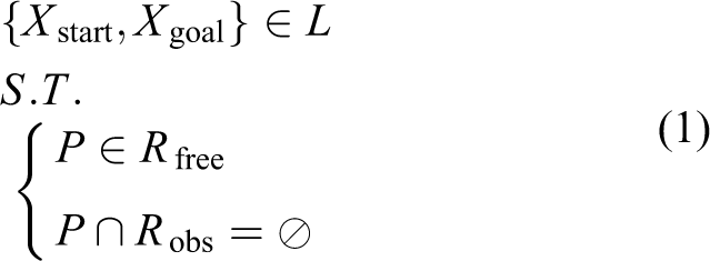
L denotes the generated path. Sensors such as laser range finders and cameras vary with respect to their accuracy under changing states. Thus, the configuration of the robot will often be imperfect (see Figure 1(a)), which means that the accurate boundaries of R_obs and R_free are unknown. In addition, due to the disturbance and model errors, the generated path cannot be accurately followed, which is called control uncertainty (see Figure 1(b)). As the general path planning method leaves out these uncertainties, it cannot generate a safe path.

Figure 1.

Two main uncertain representation of UAV. (b) Dotted line is the planned path and solid line is UAV real path.

Let S be the state of the UAV and Φ be the unstable set corresponding to each state. The policy π : Φ → S is a map that prescribes an uncertain sensing set φ_i for the current state s_i. The control uncertainty corresponding to the current state s_i is Δ ⋅ y_i. Here, we address path planning under uncertainty and regard the sensing and control uncertainty combination as the obstacle region. The obstacle region can be described as R_obs + (φ_i + Δ ⋅ y_i), and the free region is R_free − (φ_i + Δ ⋅ y_i). For path planning with uncertainty, the first goal of planning under uncertainty is to find an obstacle-free path P_uncertain from X_start to X_goal, where P_uncertain ∈ (R_free − (φ_i + Δ ⋅ y_i)) and P_uncertain ∩ (R_obs + (φ_i + Δ ⋅ y_i)) = ⊘

Dynamic constrained optimization

The cost principle to extend the exploring tree directly influences the efficiency of the whole exploring process. SBAs extend the exploring tree by solving the nearest-neighbor problem, where the nearest neighbors are nodes that connect the newly sampled nodes. Classical metrics of selecting nearest nodes, particularly the parent node, adopt the integral of the cost along the path (i.e. length), time, energy, and so on. ^5,12 For RRT*, in order to guarantee asymptotic optimal, for each iteration the method selects the neighbor by applying $N_{\text{neighbor}}:=\{n_{\text{neighbor}}\in T,\Vert n_{\text{neighbor}}-x_{\text{new}}\Vert \le \gamma {(\text{log}n/n)}^{(1/d)}\}$ , ⁸ where T denotes the whole tree, n denotes the number of nodes in the tree, d denotes the dimension of the configuration space, γ is a constant that is decided by the configuration space, and N_neighbor denotes the neighbor nodes set. But this works only under the principle of Euclidean metrics, without considering the dynamic reachability, that is, the node may not be able to connect. Thus, the convergence speed is not guaranteed as presented above.

This article tries to increase the convergence speed from the dynamic reachability point of view, that is, the UAV reachability region is constrained by the steering constraints (i.e. dynamic constraints) of the vehicle. It is illustrated in Figure 2(a) that the UAV can only reach the nodes within steering reachability. Thus, for red newly sampled node in Figure 2(b), only X₂ and X₃ are possible nodes to connect, and X₁ is excluded because of its inability to reach X_new. This is caused by the fact that the actuators have limited ability, that is, $u(t+\Delta t)\in [U_t-\delta t\cdot \epsilon ,U_t+\delta t\cdot \epsilon ]$ . For a typical continuous system,

Figure 2.

Steering constraints of UAV, which decide the extending region of each state.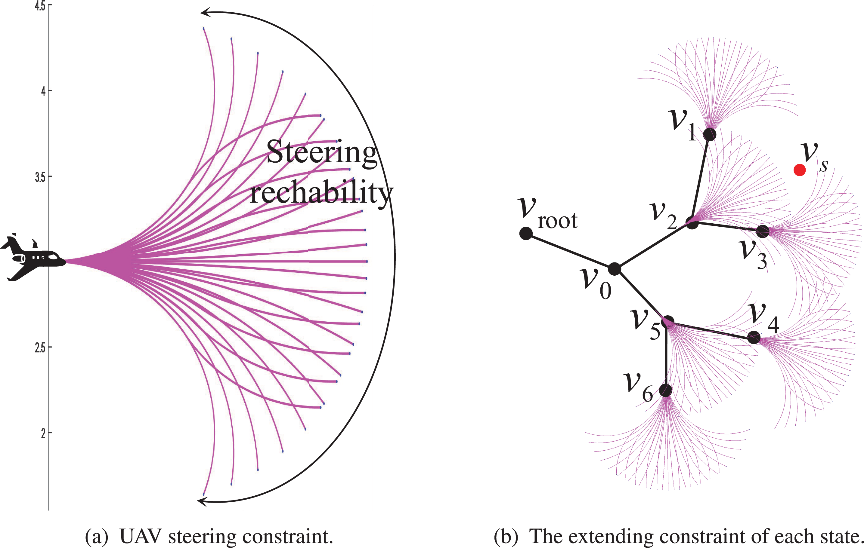

$\dot{x}(t)=f(x(t),u(t),w)$

2

Thus, x(t + Δt) can be deduced based on equation (2) and the variable control, that is, $x(t+\Delta t)\in [x(t)+f(x(t),U_t-\delta t\cdot \epsilon ,w),x(t)+f(x(t),U_t+\delta t\cdot \epsilon ,w)]$ . This indicates that the extending region is limited when applying RRTs.

Algorithms

The metric of choosing the appropriate neighbors to connect from is the bottleneck of RRTs, ¹² which must able to handle huge amount of data within limited time. The random sampling attempts are especially difficult when the environment is crowded with obstacles. ^11,20

To overcome the low exploring efficiency, we propose the dynamic concerned exploration, which is inspired by kinodynamic planning ⁵ and control effort evaluation. ¹⁹ The dynamic concerned exploration facilitates all choosing neighbors to be connectable without complex cost comparison. The redistribution method BPF is also proposed to extend with maximum amount of samplings.

Illustration of proposed GART

Pseudocode of GART is presented in algorithm 1, given the preliminary conditions: Control bounds U, initial and goal position, and initial heading at v_root, GART first samples a random state v_s (line 3), selects the possible k-nearest parents V_Neg to connect from under dynamic constraints R⁺ (line 4), v_s is redistributed under R⁺ of v_near (lines5 and 6), this article focuses using BPF to solve three events (discussed in section “Guiding steer algorithm”) and redistributes v_s or v′_s (lines 8–14) with total re-distribution vector F^v. Finally, states after re-distributed V_new will be added to the tree (line 14) with rewire (lines15 and 16). The whole process stops if the goal is reached (line 2).

GART improves general RRT* ⁸ in several ways, including the metric based on dynamics cost (lines 4, 6, and 15); the obstacles around each candidate are selected to support the BPF to redistribute the newly sampled states to reasonable position (lines 8 and 11); the final node is added to the tree, which is redistributed for safe and fast convergence (line 14). These main topics will be discussed in the following sections, and we also provide an LQG-MP inspired method to handle uncertain factors.

Algorithm 1: GART
Input:
	U	< Control input
	{νroot, νgoal}	< Initial and goal position
	ψ(νroot)	< Initial heading at νroot
1:	$T\leftarrow \left\{{\nu }_{\text{root}}\right\},R^{+}({\nu }_{\text{root}})\in R^{+}[{\theta }_{\text{root}},J_{\text{root}}]$
2:	while Not reach νgoal do
3:	νs ← StateSample()
4:	$V_{\text{Neg}}:=\left\{{\nu }_i\right|{\nu }_s\in R^{+}[\infty ,{\theta }_{{\nu }_i}],{\nu }_{i\mathrm{,...},k}\in T\}$
5:	νnear ← Nearest(VNeg, νs)
6:	Generate: ${\nu \prime }_s\leftarrow (k\prime {\nu }_{\text{near}}+k\prime {\nu }_s)$ &    ${\nu \prime }_s\in R^{+}[{\theta }_{{\nu }_{\text{near}}},J_{{\nu }_{\text{near}}}]$
7:	if CollisionFree(νnear, ν′ s ) then
8:	ν′ s = GuidingSteer(ν′ s , T)
9:	Vnew = ν′ s
10:	else if
11:	then {aνF1, aνF2} = GuidingSteer(νs, T)
12:	Vnew = {aνF1, aνF2}
13:	end if
14:	T ← InsertState(T, Vnew)
15:	$V_{\text{Neg}}:=\left\{{\nu }_i\right|{\nu }_i\in R^{+}[\infty ,{\theta }_{V_{\text{new}}}],v_{i\mathrm{,...},k}\in T\}$
16:	T ← Rewire(Vnew, VNeg)
17:	end while

Obstacle modeling with uncertainty

For path planning, the first problem is how to reconstruct the environment online with the appropriate model. Two types of methods are commonly used to model the obstacles. One is based on detailed polynomial mathematical equation to rebuild the obstacle region. ³⁰ This method requires sufficient and complex resources to describe the obstacles with much computational resources. The other methods model the obstacle region with occupancy grid, ³¹ which represents the environment in detail using large amount of cells. Ning ³² proposed a promising method called fuzzy boundaries to handle nonlinear boundaries, which is quite promising. Both are widely implemented for UAV and many other robots; however, they need more storage and time to be explored, particularly in cluttered environment with uncertainty.

This article introduces ellipse (and ellipsoid in 3-D) to model the obstacles with some promotion, which is quite commonly used and tested in real environments. ^13,33,34 We are concerned about the uncertainty of the sensors, which also affected the uncertainty of the control phase. ¹³ This article regards the sensor detection results obey Gaussian distribution (Figure 3(a)), that is

Figure 3.

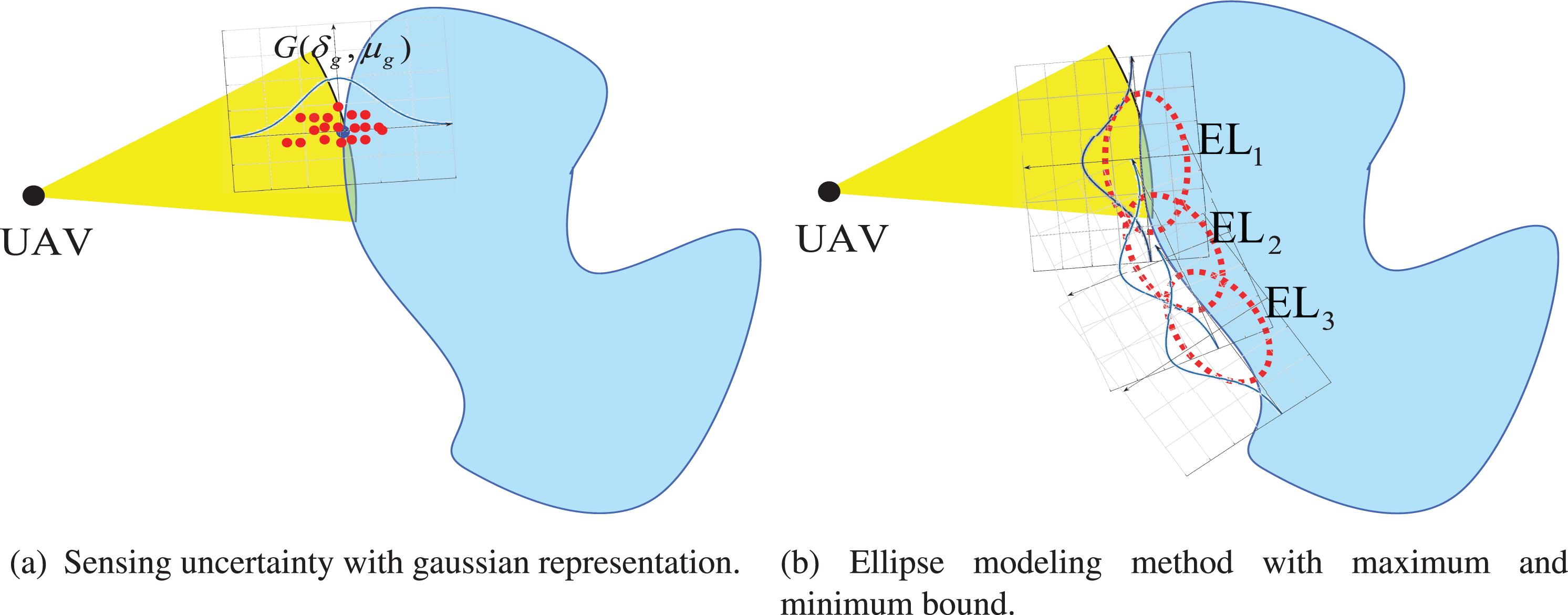
On board sensing noise is described as Gaussian noise in (a). Then inspired by LQG-MP ¹³ to calculate the margin factor of each sensed node to represent the obstacle, which are the red ellipses EL_i in (b).

$G({\delta }_g,{\mu }_g)=\frac{1}{{\delta }_g\sqrt{2\pi }}\text{exp}\left(\frac{-{(p_{x\mathrm{.}y\mathrm{.}z}-{\mu }_g)}^2}{2{\delta }_g^2}\right)$

3

μ_g denotes the center position of each sensed node or along a certain axis, δ_g is the deviate error, and p_x.y.z is the position of the node. We are inspired by LQG-MP ¹³ to calculate the distribution bound of obstacle region under uncertainty using probability. Onboard sensors are supposed to obtain Gaussian noise (equation (3)), and the probability of any node on the obstacle within O_s is

$P_{O_s}:=\Gamma (\frac{d}{2},O_s^2)$

4

Here, d is the dimension of Gaussian distribution. In order to ensure safe modeling of the obstacle, we define that for any sensed node v_KF by Kalman-filter ¹³ probability bound $P_{\text{min}}(v_{\text{KF}})\le P(v_{\text{KF}})\le P_{\text{max}}(v_{\text{KF}})$ must be kept. Based on equation (4), the maximum and minimum factors O_s can be achieved. Thus, two ellipses with different margin factors can be achieved, and this article defines the minimum factor as the intersection principle. As illustrated in Figure 3(b), ellipse EL₁ is constructed by obtaining minimum margin factor O_s(min) with EL₂. Thus, we can use less ellipse to represent the obstacle region, which can successfully decrease the memory to speed up the exploration.

Dynamic concerned exploration

To enable the post processing of the planned path, the path planners are required:

The connection between any two states must meet the dynamic constraints.

Any local connections between joints should be kept as smooth as possible.

We are inspired by numerous research works, which aim to find the most platform-adaptive and implementable extending metrics for RRTs. The LQR cost evaluated the neighbor-chosen metric, ¹⁹ expended control, and time combined cost-bounded extending, ⁵ they share the same merits of obtaining dynamic reachability. Our method also obtains a reachable region, that is, R⁺ denotes the feasible forward extending region (FER) (the illustrated region in Figure 3(a))

$R^{+}[\theta ,J]=\{v\in V\Vert x-v|\le J(\alpha )\text{and}|\alpha =a\text{cos}(v_p-v,x-v)|\le {\theta }_m\}$

5

θ_m denotes the maximum reaching angle range at each v ∈ V in 2-D (which can be easily extended to 3-D) in δt time, J(α) is farthest distance can be reached, where

$\begin{array}{ll}\hfill & {\theta }_m=\text{max}\left\{{\theta }_i\right|{\theta }_i=|a\text{cos}(g(f(x,u_i(t+\Delta t)),w)-v,v_p-v)|,v\in V\}\hfill \\ \hfill & J(\alpha )=\left\{J_i\right|J_i=|p(f(x,u_i(t+\Delta t)),w)-v|,v\in V\}\hfill \end{array}$

6

u_i(t + Δt) is described in section “Dynamic constrained optimization,” which obtains a bound in any time interval. R⁺ is a varying bound that is related to (state, control) := (X, U). For GART, unlike r = γ(logn/n)^(1/d) radius-bounded RRTs ^5,8 or k-nearest RRT, ⁸ which are analyzed in geometric aspect to obtain asymptotic optimality, it first selects k dynamic feasible parents nearest(k) based on equation (6) for newly sampled v_s. Then, we introduce the cost metric

$\begin{array}{l}{C}_v:=|[(v_s-v)\phi (v,v_s-v{)]}^{T}Q[(v_s-v)\phi (v,v_s-v)]|\hfill \end{array}$

7

φ(v, v_s − v) returns the angle between v and v_s − v. The metric is associated with control effort, where v ∈ Nearest(k). GART chose only the minimal cost vertex to connect from. From Figure 3(b), for example, v_root, v₀, v₂, and v₅ can be the parent of v_s if set k ≥ 4. Then, v₂ is chosen as the parent vertex to connect from by applying equation (5).

Guiding steer algorithm

Guiding steer is used to calculate the redistribution vector to redistribute the newly sampled vertex and thus enables the efficient extending, which is used in algorithm 1 at line 5. To discuss the algorithm, we explain this with two parts, which are BPF and redistribution vector.

BPF

BPF improved a lot of random SBAs by reusing the obstacle-collided samplings and also enables the best redistribution for nodes, which will lead to stop in front of the edge (nodes that are ended without extending region in front of obstacle region edges). In order to make BPF works, a preliminary work, which is obstacle detection and counting should be explained first.

Obstacle detection and counting

Before applying the BPF, let us first discuss the obstacle detection (i.e. environment modeling). Onboard sensors have limited sensing area, thus only obstacles within the detection range can be taken into consideration. In section Obstacle modeling with uncertainty,” we talked about using ellipse to describe the uncertainty of sensing, and these ellipse cannot cover if there exist a gap. This article defines that nodes detected are represented with (angle and position), that is, (θ(v), v). Thus, for a set of continuous nodes $V=\left\{v_i\right|v_i\in O,i=1,2,\mathrm{...}\}$ , their angle and position vary with a limited value. In order to judge the continuity of each detection period, we use the L₂ measure that any two neighbor nodes must obey $L_2:|v_i-v_{i-1}|\le J_{\text{cons}}$ , J_cons is the maximum L₂ distance that ensures continuity. It is illustrated in Figure 4, if the current detection is continuous, the system regards the existence of only one obstacle confronted (Figure 4(a)). The system regards the existence of many obstacles if the detection is discontinuous (Figure 4(b)).

Figure 4.

The obstacle detection algorithm regards there exists an obstacle if a continuous edge is detected. It cannot distinguish the gap within a obstacle and regards them as two obstacles.

BPF does not simply introduce the PF to slightly adjust the position of the sampling as employed in the study by Qureshi et al. ²⁹ and it tries to obtain active exploring ability for algorithms. Based on the work of Qureshi et al, ²⁹ it just simply introduces the obstacle support repulsion and the goal support attraction, that is

$\{\begin{array}{l}{U}_{\text{rep}}\propto {\displaystyle \sum _{i=0}^m}\frac{1}{J(v_s,v_{O_i})}\\ U_{\text{rep}}\propto J(v_s,v_{\text{goal}})\end{array}$

8

As J(v_s, v_Oi) < J_dm, where J_dm denotes the maximum detection range, thus repulsion ^OU_rep existed for detected obstacles confronted. Fusing this with RRT seems promising, but there are two problems: (1) The newly sampled v_s always get repulsion from the nearby obstacles, thus if there is a narrow corridor, the chance of going through decreases. From Figure 4(b), for example, if there exist a corridor between cl₁ and cl₂, method adpoted by Qureshi et al. ²⁹ fails. (2) The method still neglects the nodes in collision, which thus waste more time in collision detection and sampling.

As illustrated in Figure 5(a), the PF is easy to achieve. But the repulsion of obstacles provides the force to move the sampling away. BPF introduces bidirectional potential for obstacles, that is, the inner involves repulsion to make the newly sampling out, and the outer involves attraction to support active exploring in crowded. It can be represented as

Figure 5.

BPF is introduced unlike general APF (a), which makes the inner with repulsion and outer with attraction (b). BPF: bidirectional potential field; APF: artificial potential field.

$\{\begin{array}{l}{}^O{U}_{\text{rep}}^{+}\propto -J(v_s,v_O)\\ {}^O{U}_{\text{rep}}^{-}\propto {\displaystyle \sum _{i=0}^m}J(v_s,v_{O_i})\end{array}$

9

${}^O{U}_{\text{rep}}^{+}$ denotes the inner repulsion, which is only decided by the obstacle O in which it locates. ${}^O{U}_{\text{rep}}^{-}$ means attraction of the outer side, which is related to all nearby obstacles O := {O_i|i = 1, 2, ... }.

Redistribution vector

BPF introduces ${}^O{U}_{\text{rep}}^{+}$ and ${}^O{U}_{\text{rep}}^{-}$ and leverages these to guide the newly sampled nodes for active and safe exploration. Redistribution Vector is a purposely defined factor to adjust the state with inappropriate location, which works like Support Vector Learning to provide more information for exploration. ³⁷ It obtains repulsion ^Of^v+ and attraction ^Of^−v vectors, which focus on inner collided and outer not good located states separately. Guiding steer vector is calculated and returned by one of the following three events:

When newly sampled state v_s (the red node) locates in dangerous region, this attempt to find the state in same direction is inappropriate even if ${}^O{U}_{\text{rep}}^{+}$ tries to push it to collision state (the blue node). As illustrated in the redistribution in Figure 6(a), collision detection is executed within the reachable range θ, which is calculated based on R⁺[θ, J] in equation (5). The first two candidate states ^a v₁ and ^a v₂, which are just out of collision or still collide at R⁺[θ, J] margin, are chosen to be connected.

Every time a new state v_s is sampled, which is located in the collision-free region and can be connected, the neighbor obstacles are detected and counted by applying BPF (described in section “BPF.”). If the number of the obstacles, ^O N, exceeds one ^O N ≥ 1 (see Figure 6(b)). v_s tries to find the nearest states ( ^O v_a and ^O v_b in Figure 6(b)) on the nearby obstacles, respectively. For this situation, it is called attraction.

A special case of the second event is that ^O N = 1, the method in event 1 is still applicable. Attraction is reversed to become repulsion and thus enables the sampled or redistributed states generated by event 1 to stay in collision-free and re-extendable state.

Figure 6.

When any new sampled state located in dangerous region, two reachable states, which are collision free, are chosen as candidates (a). Then for all states in safe region with multi-obstacles crowded are redistributed by using attracting force (b).

We hereafter discuss the process of generating redistribution vector in detail. Consider v_s is sampled randomly, the previous whole state tree T := {v_i, i = 1, 2, ... }, where v₁ = v_root. v_s tries to find the nearest state v_near among all the reachable neighbors ${}^{r}N:=\left\{v_i\right|\phi (v_s,v_i,v_i^p)\le \theta ,i=1,2,\mathrm{...}\}$ . Where θ = θ_m that is calculated based on equation (6). For v_nearest

$\begin{array}{l}{v}_{\text{near}}:=\text{min}\left\{C_{v_i}\right|v_i{\in }^{r}N\}\hfill \end{array}$

10

Then let us consider event 1, if v_s is in collision as illustrated in Figure 6(a), the extending along the same direction is presented as the blue state ∈ R⁺(v_near), which is generally adopted or just resampled. Discussion and comparison will be given later. We note that every sampling is useful and extendable, two new states (^av₁ and ^av₂) that are out of collision or with maximum turning angle are selected

$\begin{array}{l}{\{}^a{v}_1{,}^a{v}_2\}\in R^{+}\\ S\mathrm{.}T\\ {\{}^a{v}_1{,}^a{v}_2\}\cap O=\oslash \\ or\phi {(}^a{v}_i,v_{\text{near}},v_{\text{near}}^p)=\theta ,J{(}^a{v}_i)=\text{max}J(\theta )\end{array}$

11

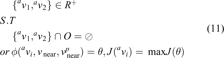
Here, the second constraint is to define that the state should be collision free, and the second constraint defines that the turning angle is the maximum, maxφ = θ, if none or only one collision free can be found. J(^av_i) = maxJ(θ) denotes the maximum distance can be reached. Thus, the redistribution with repulsion is

$\begin{array}{l}{}^v{f}_1{:=}^a{v}_1-v_s\\ {}^v{f}_2{:=}^a{v}_2-v_s\end{array}$

12

Still for event 1, if v_s can connect to v_near successfully without collision, we only execute reachable extension in the same direction v_near → v_s within R⁺(v_near). The newly generated candidate is ${}^a{v}_3:=v_{\text{near}}+(J(\phi (v_s,v_{\text{near}},v_{\text{near}}^p))/L_2(v_{\text{near}}-v_s))\cdot (v_s-v_{\text{near}})$ based on “Dynamic concerned exploration” section, thus

${}^v{f}_3{:=}^a{v}_3-v_s$

13

However, ^vf₃ is not repulsion as ^vf₁ or ^vf₂, which is the accessible state with fixed direction within R⁺. Now, the possible candidate states are selected that subject to dynamical constraints. Guiding attraction, which is exactly the main method proposed by this article to enable active exploration through obstacle-crowded environment. Two situations are discussed separately in events 2 and 3, let us first discuss event 2 where multi-obstacles exist (a simple illustration is given in Figure 6(b)). We define that the obstacles support attraction to the state, for each obstacle, the nearest node ^Ov_i margin node is selected among all the margin nodes (the red nodes) within detection range. Again, we define the attraction is proportional to the L ₂ norm of ^Ov_i−^av_j, which is

${}^a{f}_i:=k_1\cdot L_2{(}^O{v}_i{-}^a{v}_j)$

14

Thus, the total attraction is

${}^{a}f:=k_1{\displaystyle \sum _i^a}{f}_i=k_1{\displaystyle \sum _i}{L}_2{(}^O{v}_i{-}^a{v}_j)$

15

Here, k₁ is the same as the scale of the magnitude of the attraction for all candidate states. a_f denotes the total forces to redistribute the candidate ^av_j. But if only one obstacle is nearby, the attraction is reversed to become repulsion ^av_j, we define the magnitude is reverse to the distance to the nearest margin node ^Ov_i. Thus, the repulsion vector is

${}^{r}f:=k_2{\cdot }^{r}m\cdot {(}^O{v}_i{-}^a{v}_j)$

16

Here ${}^{r}m:=k_2\cdot 1/L_2{(}^O{v}_i{-}^a{v}_j)$ which denotes the magnitude of the repulsion vector, k₂ is a scale to balance the magnitude of the repulsive force. ^rf redistributes the candidate for event 3.

Finally, we still apply the goal attraction ${}^a{f}_g:=k_3\cdot L_2(v_g{-}^a{v}_j)\cdot (v_g{-}^a{v}_j)$ to enable goal-biasing ability, this accelerates the whole exploring process of the algorithm. By applying all above guiding attraction, v_s is now with the redistribution vector

$F^v{=\{}^v{f}_i{+}^{j}f{+}^a{f}_g\}$

17

Here, F^v denotes the final redistributed nodes set, i ∈ {1, 2, 3}, which is discussed in equations (12) and (13), j ∈ {a, r} that is discussed in equations (15) and (16).

Algorithm comparison and analysis

In this section, we demonstrate that GART has better performance than RRT and RRT* in completeness and convergence ability. The two most important properties of GART are completeness and convergence ability. We analyze the probability completeness of GART, which guarantees whether the final feasible path can be achieved. Asymptotic convergence ability is also analyzed and compared with RRT*.

For further discussion, the following notations are presented based on the work of Karaman: (1) The RRT algorithm is not asymptotically optimal and (2) RRT* and RRT represent probabilistic completeness. In this article, in order to keep the flow of the presentation, the proofs of important thorems are presented in the Appendix .

Convergence analysis

GART is based on Monte Carlo sampling method and has its own special properties. Thus, its convergence ability must be analyzed to prove that GART can guarantee global convergence.

Probabilistic completeness

LaValle et al. proved that the probability that RRT can find a feasible path from start to goal approaches 1 when the number of iterations approaches infinity. GART is based on RRT*, and outperformed RRT* using samples in collision to generate extra extendable samples, which ensures higher probability to expand the tree.

Theorem 4.1 (completeness of GART)

Given initial condition (x_start, x_goal, and W), GART is able to solve the path planning problem. When there exists a b > 0 and n₀inN, the probability is such that

$P{(}^{\text{GART}}{V}_n\cap x_{\text{goal}})>1-e^{-bn}\ge P{(}^{\text{RRT}*}{V}_n\cap x_{\text{goal}}),\forall n>n_0$

18

Here b and n₀ are constant that dependent only on R_free and R_goal (the goal region). For proof of this theorem, it can be found in Appendix 1.

Asymptotic optimal

For RRT*, it has to choose the best parent within the appropriate ball range γ_RRT*, that is, RRT* must have a new node that is no longer than γ_RRT* away for extending. RRT* guarantees convergence to the asymptotic optimal with ${\gamma }_{\text{RRT}*}>(2(1+1/d)1/d)(\mu (R_{\text{free}})/L_d)1/d$ . ⁸ Note that, L_d is the Lebesgue measure (i.e. volume) of the unit d-dimensional ball and μ denotes the Lebesgue measure function.

GART obtains change in the sampling distribution, while in order to analyze asymptotically optimal, let us first discuss the following notations: (1) notice the reality for the optimal path that is based on the minimal cost exist, and let S_δ denotes the length of the optimal path δ, γ_GART denotes the neighbour chosen radius; (2) to guarantee optimal, the optimal path δ must cover a number of d-dimension balls B (with γ_δ radius), and each neighbor balls are assumed to have a overlapping range αγ_δ; and (3) the path obtains γ clearance for all balls, and αγ_δ := γ/1 + ′α. Thus, the number of balls B can be computed as follows

$M=\left|B\right|\le \frac{S_i}{\alpha {\gamma }_{\delta }}\le \frac{(1+\prime \alpha )S_{\delta }}{\alpha \gamma }{\left(\frac{n}{\text{log}n}\right)}^{\frac{1}{d}}$

19

The optimal path convergence problem then can be regarded as that there exists m ∈ {1, 2, ... M} d-dimensional balls. If there exists at least a pair of nodes $x_i\in V_n^{\text{GART}}$ and $x_{i\prime }\in V_n^{\text{GART}}$ , with x_i ∈ B_m and x_i′ ∈ B_m+1 for all of the m balls, the two nodes can guarantee a connection. This event is represented by A_n and $A_n={\cap }_{m=1}^M{A}_{n,m}$ , respectively.

Theorem 4.2 (Optimality of GART)

GART is able to redistribute the samples within the consideration of increasing the convergence speed, it is asymptotically optimal for any path planning problem (x_start, x_goal, and W). It means that the cost C_n of the path of GART will finally approach an optimal solution c^finite with probability 1

$P\left(\right\{\underset{n\to \infty }{\lim }{C}_n=c^{\text{finite}}\left\}\right)=1$

20

The asymptotic condition is as follows. Detailed proof of Theorem 4.2 can be found in Appendix 2.

${\gamma }_{\text{GART}}^d>\left(2\right(1+\frac{1}{d})-\frac{L_d{\gamma }_{\text{obstacle}}^d\cdot \beta }{\mu (R_{\text{obstacle}})}{)}^{\frac{1}{d}}{\left(\frac{\mu (R_{\text{free}})}{L_d}\right)}^{\frac{1}{d}}$

21

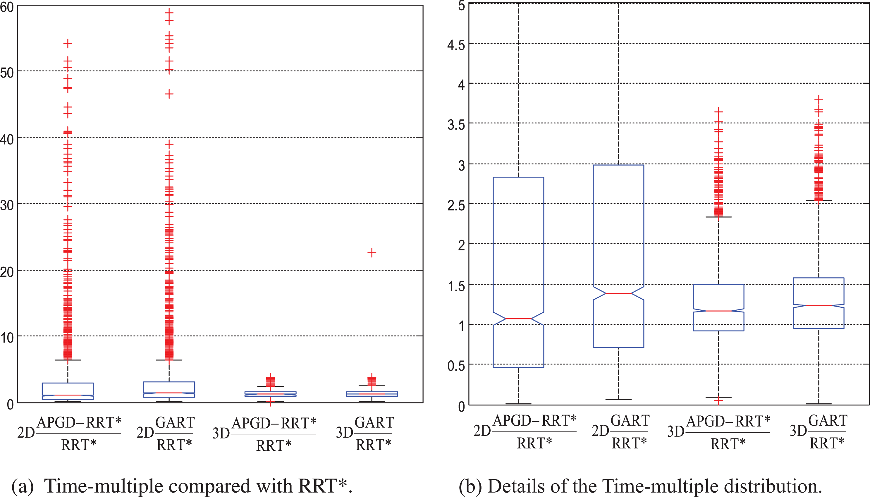
When compared with RRT*, the result shows

$\frac{{\gamma }_{\text{GART}}^d}{{\gamma }_{\text{RRT}*}^d}=\frac{{(2(1+\frac{1}{d})-\frac{L_d{\gamma }_{\text{obstacle}}^d\cdot \beta }{\mu (R_{\text{obstacle}})})}^{\frac{1}{d}}}{{\left(2\right(1+\frac{1}{d}\left)\right)}^{\frac{1}{d}}}$

22

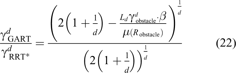
As this article models the obstacle region as ellipse in 2-D (cylindroid or ellipsoid in 3-D), that is, μ(R_obstacle) ≤ μ(ellipse), thus

$\frac{L_d{\gamma }_{\text{obstacle}}^d\cdot {\beta }^{\frac{1}{d}}}{\mu (R_{\text{obstacle}})}\ge 1$

23

Substituting equation (22) into equation (23), the result shows

$\frac{{\gamma }_{\text{GART}}^d}{{\gamma }_{\text{RRT}*}^d}\le \frac{{(1+\frac{2}{d})}^{\frac{1}{d}}}{{\left(2\right(1+\frac{1}{d}\left)\right)}^{\frac{1}{d}}}$

24

The result indicates that GART minimizes the neighbor search distance of finding best parent node (see line 11 of algorithm 1) and thus decreases much resources to execute cost comparison and collision detection of those parent nodes. This is why our GART has better performance than RRT and its variants in speeding up the convergence rate.

Computational complexity

GART holds true to the general process of RRT*, meanwhile, it introduces BPF and dynamic concerned exploration for fast convergence. According to algorithm 1, GART applies neighbor search, which obtains dynamic concerned exploration, “guiding steer,” and “nearest” search to generate the path. Based on Karaman’s work, ⁸ we may find that RRT and RRT* share the same processing time complexity O(nlogn) and the same query time complexity O(n).

Nearest searches through all n states to find k-nearest states. The dynamic constrained cost function only with the time complexity of O(1). Thus, the total time complexity is still O(logn). Guiding steer procedure is concerned with the obstacles, where the obstacle number m results the function time complexity of O(2 log ^d m). Neighbor searches all n nodes to pick our the nodes within certain distance, then its time complexity is O(logn). Thus, the total processing time is O(n(2 logn + 2 log ^d m)), which does not waste any more time than RRT*.

Experiment results

Requirements of the planner are 2-D and 3-D space with detectable obstacles. First, we illustrated the time and obstacle tackling efficiency of our active pursuing planner by providing comparisons. This can be shown by comparing the first-directive-connect (FDC) time and first-glance-connect (FGC) time. Also, we analyze the relationship between the environment scale and the exploring ability for the planner. For all simulations, they were carried out in Matlab 2013B with a Core I5 processor and 2G RAM, and the real experiment was carried out using robot operating system (ROS).

Exploring performance in cluttered environments

We design a representative map with obstacles (see Figure 7), the comparisons are carried out between RRT* and our GART. The setup is the following: we want the planner to explore in 110 × 110 space, from starting location to goal location, and we employ the unmanned ground vehicle model to represent the 2-D system model of UAV, that is

Figure 7.

Evaluation of FDC of comparative algorithms. FDC: first-directive-connect.

$\begin{array}{l}\dot{x}=vcos\cdot \vartheta \\ \dot{y}=v\cdot sion\vartheta \\ \dot{\vartheta }=\varpi \end{array}$

25

We define v = 5 m/s, ϖ = 0.2 ⋅ π, Δt = 1, Δt defines the forward extending duration for taking into consideration. Therefore, $\pm \vartheta \in [-0.2\cdot \pi \mathrm{,0.2}\cdot \pi ]$ is the variation bound of ϑ and maxJ = 5 for FER of each state.

Let us first evaluate the performance under two requests: FDC (see Figure 7(a)) and FGC (see Figure 8(a)). These two kinds of situations indicate the obstacle-crowded environment adaptive ability and exploring efficiency. Following indicators such as iterations (I), number of vertex in the tree (n), cost (C), time (t), and percentage of useful samples (POUS) are discussed in this article. FDC results of GART (Figure 7(a)), APGD-RRT* (Figure 7(b)), and RRT* (Figure 7(c)) are illustrated in Figure 7. GART introduces the BPF to redistribute sampling in FER, it enables generating of more re-extendable samples to achieve dynamic feasibility. In Figure 7(a), the blue tree is generated without using rewire as general RRT*, which is almost smooth as RRT*. The most exciting result is that GART can generate 452 states within 360 iterations, a collision state can be redistributed as one or two collision-free states toward the best extending direction and thus enables more efficient exploring. FGC results are illustrated in Figure 8(a) to 8(c). Although GART outputs with large cost path than APGD-RRT* and RRT*, it can generate a much more diverse tree with almost the same iteration, that is, the algorithm enables a higher probabilistic of completeness as well as convergence. We note that Figure 8(a) is the worst case of GART in finding FGC, and the average performance is better than other algorithms.

Figure 8.

Evaluation of FGC of comparative algorithms. FGC: first-glance-connect.

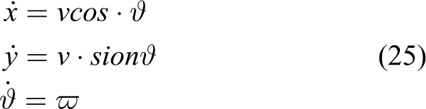
For FDC and FGC, Table 1 summarizes the main indications of each algorithm both in 2-D and in 3-D. For cluttered environments, both RRT* and APGD-RRT* are unable to fully and reasonably sample within the configuration space, this is caused by collision connect within the states. Thus, RRT* and APGD-RRT* only obtains 71% and 73.4% of useful states (POUS), while our GART can generate 127% POUS with iterations. According to this, it is also rational that GART can find the goal with average 473 iterations for FDC and 195 iterations for FGC. Time complexity are tested, we record the time for each iteration of each method, then we calculate the multiple by executing t_GART/t_RRT* and t_APGD-RRT*/t_RRT*. Result is illustrated in Figure 12, where we can deduce GART to obtain a higher time complexity than APGD-RRT* and RRT*. The medium value of time complexity of GART compared to RRT* is 1.23, while the exploration time will not increase much as the iteration efficiency is much higher than other algorithms.

Table 1.

FDC and FGC comparison between RRT*, APGD-RRT*, and GART.

Purpose	Method	I min	I max	I avg	t min	t max	t avg	C avg	POUS
FDC (Figure 7(a)	GART	360	560	473	30.87	50.95	41.14	149.1	127%
Figure 7(b)	APGD-RRT*	520	880	715	42.91	66.03	55.86	148.29	73.4%
Figure 7(c))	RRT*	720	1000	884	55.21	75.97	64.48	146.37	71%
FGC (Figure 8(a)	GART	133	249	195	10.62	22.00	16.03	159.32	–
Figure 8(b)	APGD-RRT*	240	412	326	19.98	35.5	29.24	151.65	–
Figure 8(c))	RRT*	296	409	338	17.05	26.46	22.94	154.283	–
D FDC(Figure 9(a)	GART	580	580	580	2.24	2.35	2.28	93.77	99.5%
Figure 9(b)	APGD-RRT*	1230	1230	1230	4.95	5.33	5.12	97.99	87.64%
Figure 9(c)	RRT*	2210	2210	2210	9.76	1023	9.96	104.22	79.68%

GART: guiding attraction-based random tree; RRT: rapidly exploring random tree; FDC: first-directive-connect; FGC: first-glance-connect.

Comparisons are also implemented in 3-D environment (see Figures 9 and 10). We test FDC for GART, APGD-RRT*, and RRT* and results are illustrated in Table 1 and Figure 9(a) to 9(c). The terrain-like environment contains four mountains, GART can find a way out easily by redistributing the states in danger, and thus it can reache the goal within 580 iterations for average. However, both APGD-RRT* and RRT* obtain no collision process method, they need almost 2 and 4 times time to find the path. Another advantage of the environmental information-based redistribution is that the cost can be much more smaller even at the the first time of reaching the goal, that is, c = 93.77 of GART compared with c = 97.99 of APGD-RRT*, and c = 104.22 of RRT*. We apparently see that the red path is smoother and without much turning in Figure 9(a) than Figure 9(b) and Figure 9(c).

Figure 9.

Illustration of the first arriving to the goal of GART, APGD-RRT*, and RRT*. GART: guiding attraction based random tree; RRT: rapidly exploring random tree.

Figure 10.

3-D results after 10,000 iterations, black lines indicate the tree and red line indicates the path.

As discussed earlier, the POUS is very important to indicate the efficiency of obstacle handling, here we also discuss another indicator, that is, percentage of rewire (POR). POR reveals the dispersion (or reasonable sampling rate) of the algorithm. For the 3-D environment (Figure 9), we make the methods to explore for 10,000 iterations and record the POUS and POR for each 1000 iterations. Results are illustrated in Figure 11, GART obtains an average 100% POUS (Figure 11(a)), while RRT* and APGD-RRT* obtain low efficiency for exploration. For POR, GART obtains a high percentage at the beginning (Figure 11(b)) and can also obtain a high POR at the end. Higher POR means smoother, as GART introduces the dynamic constraints and thus keeps a rational distribution of states as well as shorter path can be found for FDC. The 3-D step time is also recorded and illustrated in Figure 12, the variation between 2D and 3D is caused by the distribution of the obstacles. The time average time of GART compared to RRT* is no more than 1.5 times, while iteration efficiency is four times more. The final results after 10,000 iterations of each algorithm is illustrated in Figure 10.

Figure 11.

3-D comparison of FDC between GART, APGD-RRT*, and RRT*. FDC: first-directive-connect; GART: guiding attraction-based random tree; RRT: rapidly exploring random tree.

Figure 12.

Time multiples between GART, APGD-RRT*, and RRT*. GART: guiding attraction-based random tree; RRT: rapidly exploring random tree.

Efficiency of handling narrow corridors

Narrow corridor tests are implemented in two kinds of representative benchmarks, which are S-like tunnel (Figure 13(a)) and Bug-trap-like box (Figure 13(b)). The S-like tunnel is consisted of rectangles, which constrains the robot to pass within the corridor, and this article tries to test the efficiency of the proposed algorithm by scaling the width of this S-like tunnel. S-tunnel 1.0 means that the corridor is wide enough for robot to pass through, S-tunnel 0.5 is the moderate level of width for robot, and S-tunnel 0.3 with tight corridor is hard for robot to pass. Bug-trap-like box is also designed for robot to find a way out of the box that has a narrow corridor directly to the inner region, the width of the corridor is also scaled with the above definition with Bug-trap 1.0, 0.6, and 0.4.

Figure 13.

Two representative benchmarks that have narrow corridors, which are challenges for algorithms to find a path quickly.

Comparisons with RRT, DDRRT and RRRT are implemented within the above designed narrow corridor environments to demonstrate the ability of our algorithm. RRRT and DDRRT are all proved to be more efficient than RRT in most situations. ²⁰ For all the benchmarks, our GART spends less than the average time to find a collision-free path which at most needs 5 s to find a feasible path.

For the easy S-like tunnel, GART shows relative better performance, which are 13.1% and 6% times faster than basic RRT and RRRT. But with over 10 times faster than DDRRT (Table 2). The performance increases when the corridor is with moderate difficulty for GART, where the time decreases to find a path. In the moderate situation, the multiple of RRRT increases with 42% and more than 100% for DDRRT. For the hard-type S-tunnel, our method shows higher performance than RRT, that is, 53.8% faster than RRT. GART is also 5.8% faster to explore in the narrow situation when compared with RRRT. For all the benchmarks, DDRRT does not show good performance, which is due to the fact that DDRRT is sensitive with the radius of the obstacle-contact circles.

Table 2.

Performance comparisons with RRT, (DDRRT, and RRRT under representative environments with different difficulty level.

Model	Difficulty	Time needed to find a path				Iterations corresponding to the time
		RRT	DDRRT	RRRT	GART	RRT	DDRRT	RRRT	GART
S-tunnel 1.0	Easy	0.381 s	4.577 s	0.357 s	0.337 s	77	547	79	67
S-tunnel 0.5	Moderate	0.531 s	11.792 s	0.508 s	0.449 s	109	1292	77	69
S-tunnel 0.3	Hard	0.986 s	35.300 s	0.561 s	0.530 s	553	2513	101	87
Bug-trap 1.0	Easy	1.651 s	2.463 s	1.009 s	0.995 s	201	432	201	187
Bug-trap 0.6	Moderate	2.415 s	5.651 s	1.989 s	1.197 s	1152	1067	669	459
Bug-trap 0.4	Hard	4.601 s	16.640 s	2.961 s	1.641 s	2238	2643	896	524

RRRT: retraction-based RRT; DDRRT: dynamic-domain RRT; RRT: rapidly exploring random tree; GART: guiding attraction-based random tree.

The performance in Bug-trap boxes is illustrated in Table 2. For RRT, DDRRT, and RRRT, their time increases almost linear with difficulty, that is, the harder the narrow corridor is, the more time consumes. Time needed for GART with moderate environment increases 20.3% when compared with easy one, but only with 65% more when compared to hard environment. However, RRT and RRRT increase with 100% more time, which is even more for DDRRT. Both results illustrate that our method is not sensitive with the difficulty of the environments, particularly even faster when the environments become tighter to support more guiding. The results prove that GART can successfully tackle narrow corridor with relative good performance.

Experimental demonstration with unmanned aerial vehicle

Previous works of The City College of New York (CCNY) robotics lab have demonstrated that the control system ³⁵ is stable in indoor environment, and visual localization method ³⁶ is able to do real-time control. Here, we set three obstacles (illustrated in Figure 14(a)) in a narrow experiment space (around 2000 × 2500mm²), where the distance between each obstacle is able to let the drone to fly through. For navigation, we do not directly use the discrete nodes output by GART, that is, we use a path smoother ³⁷ to generate a smooth path with yaw continuity. Beside the obstacles, we set the quadrotor to fly around a constant speed of 0.5 m/s and the height is maintained at a constant of 330 mm, where final pose array can be found in Figure 14(a).

Figure 14.

Experiments with AscTec Pelican using visual simultaneous localization and mapping (SLAM) method to do localization.

For path planner, one of the most important issues is how to represent the environment, which directly results whether a method can be used to solve the problem. Since we use visual SLAM to do localization, we use the point clouds to act as perception. GART regards that if a cluster of clouds is confronted within safe distance, then we try to calculate the area of the obstacle to model with the method proposed in section “Obstacle modeling with uncertainty.” Thus, according to the point clouds, it is easy to get the environment information (where both orientation and position are supported). The result of our path planner is illustrated in Figure 15(a), and the tracking error is also provided in Figure 15(b) (the unit of the error is meter) with a mean error 0.06 m.

Figure 15.

Illustration of planned path using GART and its tracking error. GART: guiding attraction based random tree.

Conclusion

We propose an algorithm called GART for UAV on-line path planning under obstacle-crowded environments. GART introduces environmental information to guide the general random process of RRT*. Environmental information is in the form called “attraction,” which is inspired by the potential of artificial potential field. The algorithm based on the consumption that the obstacles can support the direction toward safety when confronted. Our algorithm focuses on UAV path planning, taking the control and sensing uncertainty into consideration. Despite the safety, GART also includes the dynamic constraints of heading punishment to guarantee smoothness. This article also provides theoretical analysis to prove the faster convergence ability of GART over RRT* and the ability of dealing with narrow corridor.

Comparisons were performed to prove searching, convergence, and narrow corridor passing ability in 2-D and 3-D environments. Results shows that GART outperforms RRT* with respect to searching and smoothing, and the 3-D comparisons illustrate that GART performs well in obstacle-filled situations. Narrow corridor passing efficiency is also tested with two kinds of benchmarks, and the results prove that GART has good performance in managing narrow corridors as well as RRRT. Finally, we did an experiment on UAV, which is much faster in flying through narrow corridor. However, as GART is based on local information, it does not offer any advantages if there are no obstacles.