Sage Journals: Discover world-class research

Abstract

In this article, an adaptive backstepping control is proposed for multi-input and multi-output nonlinear underwater glider systems. The developed method is established on the basis of the state-space equations, which are simplified from the full glider dynamics through reasonable assumptions. The roll angle, pitch angle, and velocity of the vehicle are considered as control objects, a Lyapunov function consisting of the tracking error of the state vectors is established. According to Lyapunov stability theory, the adaptive control laws are derived to ensure the tracking errors asymptotically converge to zero. The proposed nonlinear MIMO adaptive backstepping control (ABC) scheme is tested to control an underwater glider in saw-tooth motion, spiral motion, and multimode motion. The linear quadratic regular (LQR) control scheme is described and evaluated with the ABC for the motion control problems. The results demonstrate that both control strategies provide similar levels of robustness while using the proposed ABC scheme leads to the more smooth control efforts with less oscillatory behavior.

Keywords

Underwater glider adaptive backstepping control MIMO multimode motion

Introduction

Underwater gliders are increasingly being used to operate in dynamic and complex ocean environments. Trajectory tracking control is one of the most essential features required to ensure reliable and robust operation of a glider in such environments. Currently most of the operational gliders^1
–3 have implemented a simple proportional controller for heading or pitch control, but the cooperation of multiple actuators has limited the energy efficiency and control accuracy. On the other hand, single-objective control is no longer applicable to the increasing complex glider mission. Therefore it is important to develop advanced adaptive controllers to ensure the security and reliability of the underwater glider system.

Control for underwater gliders is a topic that has been widely researched in recent years. Existing controllers are typically designed to reach a desired pitch angle, velocity, or specified depth. A variety of approaches have been developed and applied to the attitude control problem. These include sliding mode control (SMC),⁴ linear quadratic regular (LQR) control,⁵ predictive control⁶ and adaptive control.^7,8 Maziyah et al.⁹ compared the proportional–integral–derivative (PID) controller and LQR controller, the results showed that the LQR controller has better performance but still needs further improvement to obtain a faster response. In predictive control,¹⁰ a decoupled adaptive control based on the linear glider model predictive is provided. In adaptive control,^11
–13 the control system is capable of self-learning and adapting to the variations of the vehicle dynamics and hydrodynamic coefficients. There are also other existing approaches, such as fuzzy control,^14,15 and inverse system control.¹⁶ In addition, Mahony¹⁷ and Allotta¹⁸ considered the attitude control in presence of magnetic disturbances in the underwater environment.

One of the common drawbacks of conventional control methods is that they are based either on the linearized model of the glider dynamics¹⁹ or the steady state solutions of the dynamic equilibrium,²⁰ which can be applied in the saw-tooth motion of the glider and single-input-single-output (SISO) control in spiral motion. However, when a glider operates in six degrees of freedom (6-DOFs), multiple-input-multiple-output (MIMO) control²¹ is required. Another limitation of the existing state of the art strategies is that the analytical steady solutions in spiral motion are extremely difficult to obtain,²² which might lead to the deviation between the desired signal and output results.

Based on the above research results, a nonlinear MIMO adaptive backstepping control (ABC) of an underwater glider system is proposed in this article. Preliminary work on this line of research, relating a SISO control scheme for a glider in saw-tooth motion has already been presented by Cao et al.²³ As an extension, the controller proposed in this article is designed based on the nonlinear glider dynamics in 6-DOFs, with multiple control objects in the design process. Then the adaptive backstepping method was used to approach a stable Lyapunov function with global asymptotic stability, thereby the actual multiple control laws of the dynamic system are obtained. With respect to the state-of-art of similar control systems, the proposed MIMO ABC avoids solving the steady-state motion equations and it is capable of achieving anticipated multimode motion.

The rest of the article is organized as follows. The glider dynamics in 6-DOFs are established in Section ‘Problem formulation’. Then the MIMO ABC controller designing process is introduced in Section ‘Controller design’. The simulation results and discussions will be drawn in Section ‘Simulation results’. The final section concludes the article.

Problem formulation

The glider dynamic model used in this study is adopted from existing work.²⁴ Since either the expressions or the expansions of the equations of the motion in 6-DOFs are tedious and complex, they will not be expressed in this study. Instead, the state-space equations will be established through reasonable simplification of the glider dynamics. The definitions of parameters and coefficients appeared in this study are listed in Table 1. Three coordinate frames are commonly used to describe the motion of underwater vehicles²⁵: inertial frame, body frame and flow frame. The body frame $e_{0} - x y z$ is established at the center of buoyancy: The x-axis coincides with the longitudinal axis; the y-axis lies in the wing plane pointing to the right; the z-axis is pointing to the bottom of the vehicle, as shown in Figure 1. The inertial coordinate frame is attached to the earth described by $E_{0} - i j k$ while the flow frame is used to describe the hydrodynamics forces and moments.

Table 1.

Definitions of variables appearing in glider motion.

Title	Physical significance
α, β	Angle of attack and slide
K	Hydrodynamic coefficients
m_h	Vehicle hull mass
m_p	Internal moving mass
R_p	Eccentric distance of the moving mass
γ	Rotation angle of the moving mass
m_b	Ballast mass (caused by the changing volume)
r _b1	The linear position of the ballast mass
g	Acceleration due to gravity
$M_{f 1}, M_{f 2}, M_{f 3}$	Added mass terms
$I_{f 1}, I_{f 2}, I_{f 3}$	Added moment of inertia
$I_{r b 1}, I_{r b 2}, I_{r b 3}$	Inertia of the rigid body
r _p1	Linear position of moving mass in body coordinates
ϕ, θ, ψ	Roll/pitch/yaw angle
p, q, r	Angular velocities in roll/pitch/yaw
$V_{1}, V_{2}, V_{3}$	Velocity components in body coordinates
V	Velocity

Figure 1.

Coordinate frames of the glider motion.

The simplification process is based on the following assumptions:

Assumption 1. Neglecting the coupled terms with minute value V₂, V₃, p, q, and r. It is because these variables are usually infinitesimal values at equilibrium and can be neglected when coupled together.

Assumption 2. V₁ = V, $\cos α = 1, sin α = V_{3} / V_{1}, \cos β = 1, sin β = V_{2} / V_{1}$ . Because V₂ and V₃ are always infinitesimal values compare to V₁.

Assumption 3. $sin α = α, sin β = β$ . The first term of the Taylor expansion is taken which has a high degree of approximation in this situation because both α and β are usually small values.

Define the state vector $x = {[φ, θ, ψ, p, q, r, V_{1}, V_{2}, V_{3}, r_{p 1}, γ, m_{b}]}^{T}$ , the input vector $u = {[{\dot{r}}_{p 1}, \dot{γ}, {\dot{m}}_{b}]}^{T}$ , and the desired output vector $y_{d} = {[θ, ψ, V]}^{T} . {\dot{r}}_{p 1}$ represents the linear velocity of the movable mass m_p, which is essentially the speed of the stepping motor; $\dot{γ}$ represents the angular velocity of the movable mass, which is essentially the speed of the steering engine in the rotary actuator; ${\dot{m}}_{b}$ represents the volume changing rate of the buoyancy engine, which is essentially the speed of the oil pump. And we choose the pitch angle θ, roll angle ϕ, and velocity V as the desired outputs because they are fundamental states to describe the motion of an underwater glider. The purpose of this study is to obtain the proper expression of u, which can guarantee the output vector y converges to its desired value

{y |}_{t = \infty} = y_{d}

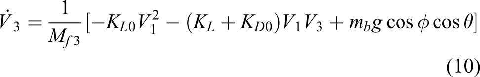
Therefore, the state-space equations of the glider system can be described by

\dot{φ} = p + q sin φ tan θ + r cos φ tan θ

\dot{θ} = q \cos φ - r sin φ

\dot{ψ} = q sin φ sec θ + r \cos φ sec θ

\dot{p} = \frac{1}{I_{f 1}} [(K_{M R} - K_{M 0}) V_{1} V_{2} + K_{p} p V_{1}^{2} - m_{p} R_{p} g \cos θ (\cos φ sin γ + sin φ \cos γ)]

\dot{q} = \frac{1}{I_{f 2}} [\begin{array}{l} V_{1} V_{3} (M_{f 3} - M_{f 1} + K_{M}) - m_{b} r_{b 1} g \cos φ \cos θ \\ - m_{p} g (r_{p 1} \cos φ \cos θ + R_{p} sin θ \cos γ) + K_{M 0} V_{1}^{2} + K_{q} q V_{1}^{2} \end{array}]

\dot{r} = \frac{1}{I_{f 3}} [V_{1} V_{2} (M_{f 1} - M_{f 2} + K_{M Y}) + m_{b} r_{b 1} g sin φ \cos θ + m_{p} g (r_{p 1} sin φ \cos θ - R_{p} sin θ sin γ) + K_{r} r V_{1}^{2}]

{\dot{V}}_{1} = \frac{1}{M_{f 1}} [- K_{D 0} V_{1}^{2} + K_{L 0} V_{1} V_{3} - m_{b} g sin θ]

{\dot{V}}_{2} = \frac{1}{M_{f 2}} [(K_{β} - K_{D 0}) V_{1} V_{2} + m_{b} g sin φ \cos θ - r V_{1} (m_{b} + m_{p} + m_{r b} + M_{f 1})]

{\dot{V}}_{3} = \frac{1}{M_{f 3}} [- K_{L 0} V_{1}^{2} - (K_{L} + K_{D 0}) V_{1} V_{3} + m_{b} g \cos φ \cos θ]

{\dot{r}}_{p 1} = u_{1}

\dot{γ} = u_{2}

{\dot{m}}_{b} = u_{3}

Controller design

This section proposes a nonlinear adaptive backstepping control law to steer the glider towards the desired output vector, and an LQR controller is introduced to compare with the proposed method.

LQR controller design

LQR is a method in modern control theory that uses state-space equations to analyze the system. The standard optimal principle is to produce a stabilizing control law that minimizes a cost function J, which is weighted by the quadratic sum of the states and input variables.²⁶ By determining the feedback gain matrix, the trade-off between the control effort, the magnitude, and the response can be established, which will guarantee the stability of the system. The cost function to be minimized is defined as

J = \int_{0}^{t_{f}} [x^{T} (t) Q x (t) + u^{T} R u (t)] d t

where Q is a symmetric positive semi-definite state penalty matrix, and R is a symmetric positive semi-definite control penalty matrix. By choosing proper Q and R, the glider dynamic can be well-behaved and the large motions in the movable mass and ballast mass that would exceed physical limitations will be prevented.

To design the LQR controller, the state-space equations of the glider must be linearized as follows

δ \dot{x} = A δ x + B δ u

where A is the Jacobian matrix of x, B is a sparse matrix, and

δ x = x - x_{d}

δ u = u - u_{d}

here x _d and u _d are the state vector and control vector at equilibrium state.

The corresponding control law is

u^{*} = - K (t) δ x

where K is the solution to the Riccati equation with given A, B, Q, and R.

The flow chart of the LQR controller is illustrated in Figure 2. The steady states are obtained through the equilibrium solver; then the time-varying control inputs can be calculated by the linearized matrix and the LQR controller. An important issue is that when the glider performs in steady spiral motion, the equilibrium states are difficult to predict. Viewing the existing steady-solutions,^27
–29 the approximated numerical solution does not match the analytic result; on the other hand, the method of numerical solution is an iterative searching process, which requires a large amount of calculations. In addition, when the glider operates in complex situations, the LQR controller is unable to adapt with time varying desired path.

Figure 2.

Flow chart of the LQR controller.

Adaptive backstepping controller design

To overcome the aforementioned difficulties in multimode control, an adaptive backstepping controller is presented in this section. The basic principle of the backstepping approach is to design a Lyapunov function reversely by applying the Lyapunov stability theory. The ultimate goal is to find a Lyapunov function whose derivative is nonpositive, so that the system reaches global asymptotic stability. ABC is usually used in a nonlinear SISO system; however, for a MIMO system, establishing the proper Lyapunov function is extremely challenging.

The control laws are designed as follows

[\begin{matrix} u_{1} \\ u_{2} \end{matrix}] = \frac{I_{f 2} I_{f 3}}{m_{p} g} A^{- 1} {[\begin{matrix} U_{1} & U_{2} \end{matrix}]}^{T}

u_{3} = \frac{M_{f 1} [c_{7} (z_{12} - c_{7} z_{7}) + c_{12} z_{12}] - 2 K_{D 0} {\dot{V}}_{1} V_{1} + K_{L 0} ({\dot{V}}_{1} V_{3} + V_{1} {\dot{V}}_{3}) - \dot{θ} m_{b} g \cos θ}{g sin θ}

where

\begin{array}{l} A = [\begin{matrix} \cos^{2} φ \cos θ I_{f 3} + {sin}^{2} φ \cos θ I_{f 2} & - (R_{p} \cos φ sin θ sin γ I_{f 3} + R_{p} sin φ sin θ \cos γ I_{f 2}) \\ sin φ \cos φ I_{f 3} - \cos φ sin φ I_{f 2} & - (R_{p} sin φ tan θ sin γ I_{f 3} - R_{p} \cos φ tan θ \cos γ I_{f 2}) \end{matrix}] \\ U_{1} = U_{11} + U_{12} + U_{13} + U_{14} + U_{15} + U_{16} + U_{17} \end{array}

\begin{array}{l} U_{11} = \frac{- \dot{φ} sin φ}{I_{f 2}} [\begin{array}{l} V_{1} V_{3} (M_{f 3} - M_{f 1} + K_{M}) - m_{b} r_{b 1} g \cos φ \cos θ \\ - m_{p} g (r_{p 1} \cos φ \cos θ + R_{p} sin θ \cos γ) + K_{M 0} V_{1}^{2} + K_{q} q V_{1}^{2} \end{array}] \end{array}

\begin{array}{l} U_{12} = \frac{\cos φ}{I_{f 2}} [\begin{array}{l} ({\dot{V}}_{1} V_{3} + V_{1} {\dot{V}}_{3}) (M_{f 3} - M_{f 1} + K_{M}) - u_{3} r_{b 1} g \cos φ \cos θ \\ - m_{p} g (- \dot{φ} r_{p 1} sin φ \cos θ - \dot{θ} r_{p 1} \cos φ sin θ + \dot{θ} R_{p} \cos θ \cos γ) \\ + \dot{φ} m_{b} r_{b 1} g sin φ \cos θ + \dot{θ} m_{b} r_{b 1} g \cos φ sin θ \\ + 2 {\dot{V}}_{1} K_{M 0} V_{1} + K_{q} \dot{q} V_{1}^{2} + 2 K_{q} {\dot{V}}_{1} q V_{1} \end{array}] \end{array}

\begin{array}{l} U_{13} = \frac{- \dot{φ} \cos φ}{I_{f 3}} [\begin{array}{l} V_{1} V_{2} (M_{f 1} - M_{f 2} + K_{M Y}) + m_{b} r_{b 1} g sin φ \cos θ \\ + m_{p} g (r_{p 1} sin φ \cos θ - R_{p} sin θ sin γ) + K_{r} r V_{1}^{2} \end{array}] \\ U_{14} = - \frac{sin φ}{I_{f 3}} [\begin{array}{l} ({\dot{V}}_{1} V_{2} + V_{1} {\dot{V}}_{2}) (M_{f 1} - M_{f 2} + K_{M Y}) + u_{3} r_{b 1} g sin φ \cos θ \\ + \dot{φ} m_{b} r_{b 1} g \cos φ \cos θ - \dot{θ} m_{b} r_{b 1} g sin φ sin θ \\ + m_{p} g (\dot{φ} r_{p 1} \cos φ \cos θ - \dot{θ} r_{p 1} sin φ sin θ - \dot{θ} R_{p} \cos θ sin γ) \\ + K_{r} \dot{r} V_{1}^{2} + 2 K_{r} {\dot{V}}_{1} r V_{1} \end{array}] \end{array}

U_{15} = - (q sin φ + r \cos φ) (\begin{array}{l} \dot{p} + \dot{q} sin φ tan θ + \dot{φ} q \cos φ tan θ \\ + \dot{θ} q sin φ {sec}^{2} θ + \dot{r} \cos φ tan θ \\ - \dot{φ} r sin φ tan θ + \dot{θ} r \cos φ {sec}^{2} θ \end{array})

U_{16} = - \dot{φ} (\dot{q} sin φ + \dot{φ} q \cos φ + \dot{r} \cos φ - \dot{φ} r sin φ)

U_{17} = c_{2} ({\dot{z}}_{5} - c_{2} {\dot{z}}_{2}) + c_{5} {\dot{z}}_{5} + c_{10} z_{10}

U_{2} = U_{21} + U_{22} + U_{23} + U_{24} + U_{25} + U_{26} + U_{27}

U_{21} = \dot{q} (\dot{φ} \cos φ sec θ + \dot{θ} sin φ sec θ tan θ)

U_{22} = \frac{sin φ sec θ}{I_{f 2}} [\begin{array}{l} ({\dot{V}}_{1} V_{3} + V_{1} {\dot{V}}_{3}) (M_{f 3} - M_{f 1} + K_{M}) - u_{3} r_{b 1} g \cos φ \cos θ \\ + \dot{φ} m_{b} r_{b 1} g sin φ \cos θ + \dot{θ} m_{b} r_{b 1} g \cos φ sin θ - m_{p} g (- \dot{φ} r_{p 1} sin φ \cos θ \\ - \dot{θ} r_{p 1} \cos φ sin θ + \dot{θ} R_{p} \cos θ \cos γ) + 2 {\dot{V}}_{1} K_{M 0} V_{1} + K_{q} \dot{q} V_{1}^{2} + 2 K_{q} {\dot{V}}_{1} q V_{1} \end{array}]

U_{23} = \dot{r} (- \dot{φ} sin φ sec θ + \dot{θ} \cos φ sec θ tan θ)

U_{24} = \frac{\cos φ sec θ}{I_{f 3}} [\begin{array}{l} ({\dot{V}}_{1} V_{2} + V_{1} {\dot{V}}_{2}) (M_{f 1} - M_{f 2} + K_{M Y}) + u_{3} r_{b 1} g sin φ \cos θ \\ + \dot{φ} m_{b} r_{b 1} g \cos φ \cos θ - \dot{θ} m_{b} r_{b 1} g sin φ sin θ + m_{p} g (\dot{φ} r_{p 1} \cos φ \cos θ \\ - \dot{θ} r_{p 1} sin φ sin θ - \dot{θ} R_{p} \cos θ sin γ) + K_{r} \dot{r} V_{1}^{2} + 2 K_{r} {\dot{V}}_{1} r V_{1} \end{array}]

U_{25} = (\begin{array}{l} \dot{p} + \dot{q} sin φ tan θ + \dot{φ} q \cos φ tan θ \\ + \dot{θ} q sin φ {sec}^{2} θ + \dot{r} \cos φ tan θ \\ - \dot{φ} r sin φ tan θ + \dot{θ} r \cos φ {sec}^{2} θ \end{array}) (q \cos φ sec θ - r sin φ sec θ)

U_{26} = (p + q sin φ tan θ + r \cos φ tan θ) (\begin{array}{l} \dot{q} \cos φ sec θ - \dot{φ} q sin φ sec θ \\ + \dot{θ} q \cos φ sec θ tan θ - \dot{r} sin φ sec θ \\ - \dot{φ} r \cos φ sec θ - \dot{θ} r sin φ sec θ tan θ \end{array})

U_{27} = [\begin{array}{l} c_{3} ({\dot{z}}_{6} - c_{3} {\dot{z}}_{3}) + c_{6} {\dot{z}}_{6} + ({\dot{z}}_{5} - c_{2} {\dot{z}}_{2}) (q sin φ + r \cos φ) sec θ tan θ \\ + (z_{5} - c_{2} z_{2}) (\dot{q} sin φ + \dot{φ} q \cos φ + \dot{r} \cos φ - \dot{φ} r sin φ) sec θ tan θ \\ + \dot{θ} (z_{5} - c_{2} z_{2}) (q sin φ + r \cos φ) (sec θ {tan}^{2} θ + {sec}^{3} θ) + c_{11} z_{11} \end{array}]

Theorem 1. The dynamic model of underwater glider are expressed as equations (2) to (13). Choose control laws given by euqations (19) and (20), the tracking error of state-space vector converges to zero asymptotically for any initial position.

Proof. The following steps will be considered.

Step 1

Define

z_{1} = φ - μ_{1}

z_{2} = θ - y_{1 d}

z_{3} = ψ - y_{2 d}

z_{4} = p - μ_{2}

z_{5} = q - μ_{3}

z_{6} = r - μ_{4}

z_{7} = V_{1} - y_{3 d}

z_{8} = V_{2} - μ_{5}

z_{9} = V_{3} - μ_{6}

z_{10} = r_{p 1} - μ_{7}

z_{11} = γ - μ_{8}

z_{12} = m_{b} - μ_{9}

where μ_i is the estimated value, and z_i is the tracking error between the state value and its estimated value (or desired value). Establish the Lyapunov function of the glider system as

V = \sum_{i = 1}^{12} \frac{1}{2} z_{i}^{2}

The objective is to find the proper control vector u, which makes the derivative of V nonpositive

\dot{V} = \sum_{i = 1}^{12} z_{i} {\dot{z}}_{i} \leq 0

Step 2

Considering equation (8), let

{\dot{z}}_{7} = {\dot{V}}_{1} - {\dot{y}}_{3 d} = z_{12} - c_{7} z_{7}

where c_i is a constant value, similarly hereinafter. The expression of z₁₂ can be obtained

z_{12} = \frac{1}{M_{f 1}} [- K_{D 0} V_{1}^{2} + K_{L 0} V_{1} V_{3} - m_{b} g sin θ] + c_{7} z_{7}

Take a derivative of equation (36) on both sides

{\dot{z}}_{12} = \frac{1}{M_{f 1}} [- 2 K_{D 0} {\dot{V}}_{1} V_{1} + K_{L 0} ({\dot{V}}_{1} V_{3} + V_{1} {\dot{V}}_{3}) - {\dot{m}}_{b} g sin θ - \dot{θ} m_{b} g \cos θ] + c_{7} {\dot{z}}_{7}

In equation (37), ${\dot{m}}_{b}$ is defined as u₃, the expressions of ${\dot{V}}_{1}, {\dot{V}}_{3}, and \dot{θ}$ have been described in equation (8), equation (10) and equation (3), and assume

{\dot{z}}_{12} = - c_{12} z_{12}

Substituting equation (38) into equation (37), the expression of u₃ is obtained (equation (20)).

Step 3

Then consider equation (3), assume

{\dot{z}}_{2} = \dot{θ} - {\dot{y}}_{1 d} = z_{5} - c_{2} z_{2}

Take derivative of the equation on both sides

{\dot{z}}_{5} = \dot{q} \cos φ - \dot{φ} q sin φ - \dot{r} sin φ - \dot{φ} r \cos φ + c_{2} (z_{5} - c_{2} z_{2})

Assume

{\dot{z}}_{5} = z_{10} - c_{5} z_{5}

Therefore, the expression of z₁₀ is obtained

z_{10} = {\begin{array}{l} \frac{\cos φ}{I_{f 2}} [\begin{array}{l} V_{1} V_{3} (M_{f 3} - M_{f 1} + K_{M}) - m_{b} r_{b 1} g \cos φ \cos θ + K_{q} q V_{1}^{2} \\ - m_{p} g (r_{p 1} \cos φ \cos θ + R_{p} sin θ \cos γ) + K_{M 0} V_{1}^{2} \end{array}] \\ - \frac{sin φ}{I_{f 3}} [\begin{array}{l} V_{1} V_{2} (M_{f 1} - M_{f 2} + K_{M Y}) + m_{b} r_{b 1} g sin φ \cos θ \\ + m_{p} g (r_{p 1} sin φ \cos θ - R_{p} sin θ sin γ) + K_{r} r V_{1}^{2} \end{array}] \\ - (p + q sin φ tan θ + r \cos φ tan θ) (q sin φ + r \cos φ) + c_{2} (z_{5} - c_{2} z_{2}) + c_{5} z_{5} \end{array}}

Again, assume

{\dot{z}}_{10} = - c_{10} z_{10}

and take derivative of z₁₀, the linear equation with two control inputs is obtained

U_{1} = m_{p} g (u_{1} \cos φ \cos θ - u_{2} R_{p} sin θ sin γ) (\frac{\cos φ}{I_{f 2}} + \frac{sin φ}{I_{f 3}})

Step 4

Using the same procedure as with equation (4), the expression of z₆ can be obtained

z_{6} = q sin φ sec θ + r \cos φ sec θ + c_{3} z_{3} - {\dot{y}}_{2 d}

where ${\dot{y}}_{2 d}$ is the changing rate of the heading angle. When the vehicle is in steady spiral motion, ${\dot{y}}_{2 d}$ is a constant value. Then assume

{\dot{z}}_{6} = z_{11} - c_{6} z_{6}

Therefore, the expression of z₁₁ is obtained

z_{11} = {\begin{array}{l} \frac{sin φ sec θ}{I_{f 2}} [\begin{array}{l} V_{1} V_{3} (M_{f 3} - M_{f 1} + K_{M}) - m_{b} r_{b 1} g \cos φ \cos θ \\ - m_{p} g (r_{p 1} \cos φ \cos θ + R_{p} sin θ \cos γ) \\ + K_{q} q V_{1}^{2} + K_{M 0} V_{1}^{2} \end{array}] \\ + \frac{\cos φ sec θ}{I_{f 3}} [\begin{array}{l} V_{1} V_{2} (M_{f 1} - M_{f 2} + K_{M Y}) + m_{b} r_{b 1} g sin φ \cos θ \\ + m_{p} g (r_{p 1} sin φ \cos θ - R_{p} sin θ sin γ) + K_{r} r V_{1}^{2} \end{array}] \\ + \dot{φ} (q \cos φ sec θ - r sin φ sec θ) \\ + (z_{5} - c_{2} z_{2}) (q sin φ sec θ tan θ + r \cos φ sec θ tan θ) + c_{3} (z_{6} - c_{3} z_{3}) + c_{6} z_{6} \end{array}}

Again, assume

{\dot{z}}_{11} = - c_{11} z_{11}

and take a derivative of z₁₁, the linear equation with two control inputs is obtained

U_{2} = m_{p} g sec θ (u_{1} \cos φ \cos θ - u_{2} R_{p} sin θ sin γ) (\frac{sin φ}{I_{f 2}} - \frac{\cos φ}{I_{f 3}})

Step 5

In equations (44) and (49), the control inputs u₁ and u₂ are the only two unknown variables, while U₁ and U₂ are related to u₃ (see from the explanation for equation (19)). Consider u₃ as a known parameter, and by solving these two joining equations, the final control laws of u₁ and u₂ can be obtained.

Note that the final control law u is irrelevant with z₁, z₄, z₈, and z₉, therefore, assume

z_{1} = z_{4} = z_{8} = z_{9} = 0

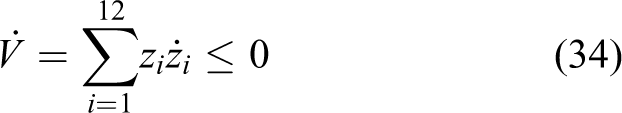
Finally, the Lyapunov function of the glider system is obtained

V = \frac{1}{2} z_{2}^{2} + \frac{1}{2} z_{3}^{2} + \frac{1}{2} z_{5}^{2} + \frac{1}{2} z_{6}^{2} + \frac{1}{2} z_{7}^{2} + \frac{1}{2} z_{10}^{2} + \frac{1}{2} z_{11}^{2} + \frac{1}{2} z_{12}^{2}

Theorem 2. By choosing proper coefficients c_i , the glider system reaches global asymptotic stability.

Proof. The derivative of the Lyapunov function V is

\begin{array}{l} \dot{V} = z_{2} {\dot{z}}_{2} + z_{3} {\dot{z}}_{3} + z_{5} {\dot{z}}_{5} + z_{6} {\dot{z}}_{6} + z_{7} {\dot{z}}_{7} + z_{10} {\dot{z}}_{10} + z_{11} {\dot{z}}_{11} + z_{12} {\dot{z}}_{12} = - c_{2} z_{2}^{2} + z_{2} z_{5} - c_{5} z_{5}^{2} + z_{5} z_{10} - c_{10} z_{10}^{2} - c_{3} z_{3}^{2} + z_{3} z_{6} - c_{6} z_{6}^{2} + z_{6} z_{11} - c_{11} z_{11}^{2} - c_{7} z_{7}^{2} + z_{7} z_{12} - c_{12} z_{12}^{2} \leq (0.5 - c_{2}) z_{2}^{2} + (1 - c_{5}) z_{5}^{2} + (0.5 - c_{10}) z_{10}^{2} + (0.5 - c_{3}) z_{3}^{2} + (1 - c_{6}) z_{6}^{2} + (0.5 - c_{11}) z_{11}^{2} + (0.5 - c_{7}) z_{7}^{2} + (0.5 - c_{12}) z_{12}^{2} \end{array}

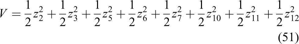
It is obvious that if the proper coefficients $c_{i} \geq 0.5 (i = 2,3,7,10,11,12), c_{i} \geq 1 (i = 5, 6)$ are chosen, the value of equation (52) is capable of remaining nonpositive. According to Lyapunov stability theory, the dynamic system reaches global asymptotic stability. This ends the proof of both Theorem 1 and Theorem 2 simultaneously.

Simulation results

To illustrate that the proposed control method is applicable to a glider system, a simulation study was carried out based on the Seawing glider,²⁰ whose mechanical properties are: $m_{h} = 54.28 kg, m_{p} = 11 kg, R_{p} = 0.014 m, I_{r b 1} = 0.6 kg \cdot m^{2}, I_{r b 2} = 15.27 kg \cdot m^{2}, I_{r b 3} = 15.32 kg \cdot m^{2}$ ; and the hydrodynamic coefficients are listed in Table 2. Multiple scenarios are considered in this section, including saw-tooth motion, spiral motion, and multimode motion. The coefficients in ABC are

c = [0,0.5,0.5,0,1,1,0.5,0,0,0.5,0.5,0.5]

Table 2.

Hydrodynamic coefficients of the Seawing glider.

List of symbol	Value
Added mass terms M_f	diag[1.48, 49.58, 65.92]
Added inertia terms I_f	diag[0.53, 7.88, 10.18]
Coefficients of drag force: $K_{D 0}, K_{D}$	7.19, 386.29
Coefficients of lift force: $K_{L 0}, K_{L}$	−0.36, 440.99
Coefficients of slide force: K_β	−115.65
Coefficients of $M_{D L 1} : K_{M R}, K_{p}$	-58.27, −19.83
Coefficients of $M_{D L 2} : K_{M 0}, K_{M}, K_{q}$	0.28, −65.84, −205.64
Coefficients of $M_{D L 3} : K_{M Y}, K_{r}$	34.10, −389.30

and the parameters in LQR controller is selected as follows

Q = diag [0.1,1,1,2,0.5,1,2,2,0.1,1,1,1,1,2]

R = diag [1, 1, 1]

These LQR parameters are developed from existing work⁵, minor changes have been made by trial and error to adapt the difference of parameters in the glider model.

Case 1: saw-tooth motion

First of all, the saw-tooth motion scenario is considered, assume the desired saw-tooth path is:

V_{d} = 0.4 m/s

ξ_{d} = {\begin{array}{l} - 0.8 / r a d & (t < 1000 s) \\ 0.8 / r a d & (t \geq 1000 s) \end{array}

where ξ = θ − α is the gliding path angle.

Figure 3 presents the pitch angle (a) and velocity (b) of the glider in saw-tooth motion with an ABC and a LQR controller, respectively. Analyzing the tracking error data, the absolute errors converge to 0 in both controllers. It can be observed that in Figure 3(a), the two controllers almost reach the steady state simultaneously. In velocity control, the LQR controller has a faster response with obvious overshoot at the switching stage; while the velocity with ABC changes smoothly to the desired value.

Figure 3.

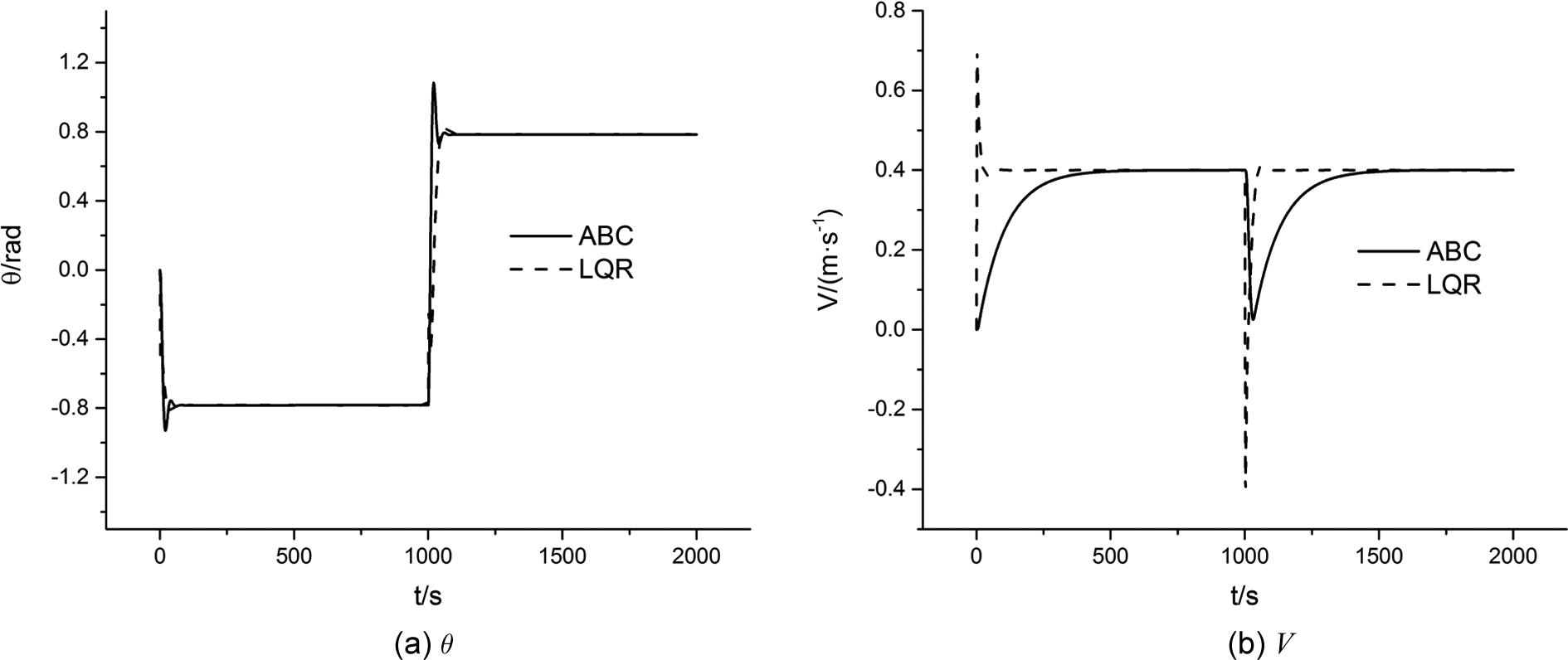
Simulated outputs of the saw-tooth motion.

The corresponding control inputs of the saw-tooth motion are illustrated in Figure 4, including the linear actuator r_p1 in Figure 4(a) and ballast mass m_b in Figure 4(b). The difference can be barely observed in r_p1, but the two controllers perform significantly differently in m_b. The LQR controller acts a fast response at the initial state of simulation, with an overshoot of 36.3%; at the switching stage, the overshoot increases to 89.7%. However, in m_b control, the ABC presents a smooth approach to the equilibrium value, without overshoots and vibrations. LQR has more overshoot, while ABC is much slower. The overshoots of the actuator will lead to additional energy consumption, which is of crucial importance in a realistic glider mission. Therefore, the ABC shows a better energy saving capability compared with the LQR in saw-tooth motion.

Figure 4.

Simulated control inputs of the saw-tooth motion.

Case 2: spiral motion

Besides saw-tooth motion, underwater gliders can perform another steady motion, which has a trajectory as a spiral. Choose the desired path

V_{d} = 0.4 m/s

ξ_{d} = - 0.8 rad

R_{d} = 200 m

where R_d is desired turning radius, which is related with the other state values

R = \frac{V \cos (θ - α)}{\dot{ψ}}

Figure 5 presents the path angle (a), heading angle (b), and velocity (c) of the glider in spiral motion with an ABC and a LQR controller. In Figure 5(a), the LQR controller reaches the desired value in a short period of time, but the tracking error still exists (0.01869 rad); the ABC overshoots the desired value by 92.6%, nevertheless, the tracking error is eliminated slowly. More distinct comparisons of the tracking ability can be observed in Figure 5(c), the ABC reaches the desired value smoothly without tracking error and overshoots; while the LQR controller has a fast converge speed at the initial stage, but the ultimate tracking error remains at 0.0275 m/s. In Figure 5(b), both the tracking error of the ABC and LQR controller exists because the heading angle ξ is not a constant. As can be seen from Figure 5(b), it is admitted that the ABC controller output is further away from the desired angle and seems not converging. However this is compensated by the fact that ABC scheme leads to less energy consumption as revealed from Figure 6. By comparing the control inputs, it is observed that the curves of the ABC scheme are more smooth compared with those of the LQR scheme, which indicates that using the ABC scheme leads to less oscillatory behavior of control efforts, and consequently leads to less energy consumption.

Figure 5.

Simulation results of spiral motion. (a) ξ. (b) ψ. (c) V.

Figure 6.

Simulated control inputs of the steady spiral motion

The trajectories of the desired path and simulation results are illustrated in Figure 7. It is obvious that the ABC path maintains a certain distance from the desired path in steady motion, while the LQR path deviates from the desired path from the beginning of the motion. In fact, the simulation turning radius of the ABC is R = 199.7 m, while the turning radius of the LQR is R = 183.1 m. The horizontal position along with operating depth is illustrated in Figure 8, the position with ABC follows the desired value with a certain deviation, while the tracking error with LQR increases along with the depth. In general, although the tracking error of trajectory in the motion still exists, the three control objects in spiral (R, V, and ξ) have been successfully tracked using the proposed method.

Figure 7.

Trajectories of the desired path and simulation results in spiral motion.

Figure 8.

Horizontal position versus depth in spiral motion.

Case 3: multimode motion

In an actual mission, a glider is usually required to complete complicated motion that combines saw-tooth motion and spiral motion. Define the multimode motion

θ_{d} = {\begin{array}{l} - 0.9 rad & t s < 4500 \\ 0.5 rad & t s \geq 4500 \end{array}

ψ_{d} = {\begin{matrix} 0 rad & t s < 1000 \\ 0.0016 t rad & 1000 \leq t s < 5000 \\ 8 rad & 5000 \leq t s < 7000 \\ 7 rad & t s \geq 7000 \end{matrix}

V_{d} = {\begin{array}{l} 0.4 m/s & t s < 2000 \\ 0.3 m/s & t s \geq 2000 \end{array}

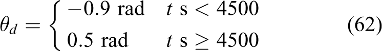
Figure 9 presents the pitch angle Figure 9(a), heading angle Figure 9(b), and velocity Figure 9(c) of the glider in multimode motion with an ABC. The motion consists of saw-tooth motion, spiral motion, turning motion,³⁰ velocity change, and path angle change. Although the motion is complicated, the tracking error barely exists in the pitch angle and velocity control no matter how the desired value changes. In the heading angle control, the tracking error converges to zero in spiral motion and turn motion. While in steady spiral motion, the tracking error of the actual heading angle exists, it is because the desired heading angle is time-variable, the simulation result is always in the approaching situation. That is because conventional underwater gliders do not have propulsion systems, the yaw motion is actuated through the rotation of an internal mass (m_p), which is much smaller than the vehicle hull mass (m_h). Another important factor is caused by the geometry shape of the vehicle, the glider has a relatively large added inertia term in yaw motion (see Table 2). These two factors lead to poor maneuverability of a glider, and the heading angle is always chasing the desired value.

Figure 9.

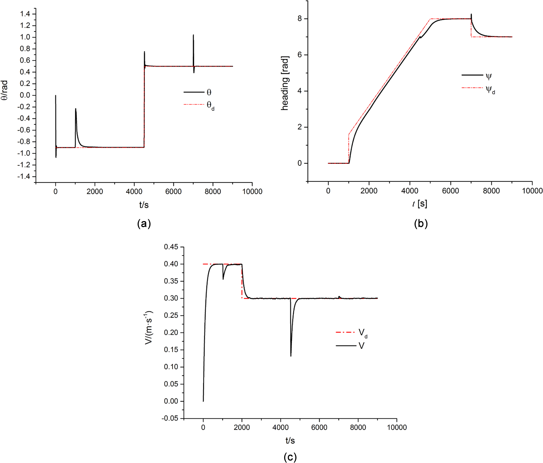
Simulation results of multimode motion with ABC. (a) θ. (b) ψ. (c) V.

The trajectories of the desired path and simulation results are illustrated in Figure 10. The simulation result coincides with the desired path at the beginning and ending stages, nevertheless significant tracking error can be observed during the spiral motion stage. The work presented in this paper primarily focuses on the attitude and velocity control, previous work has been done on studying the control strategies that drive the vehicle to the desired planned trajectories,^31,32 we believe the tracking error displayed in Figure 10 can be improved by taking use of those previous works to implement the path following control methods.

Figure 10.

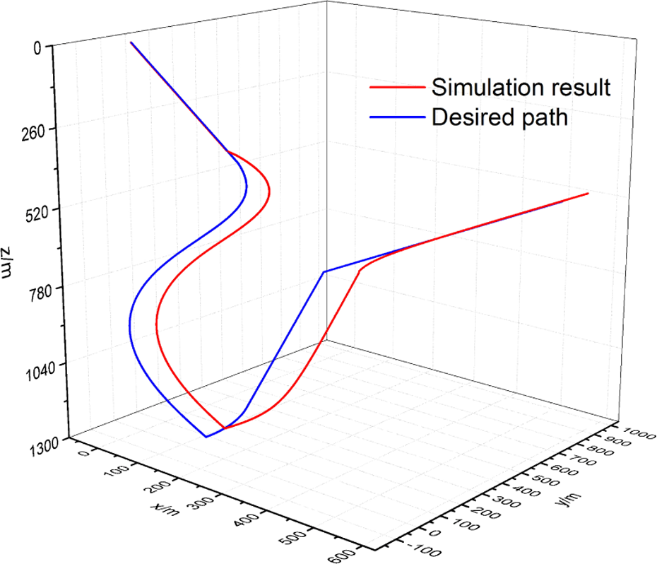
Trajectories of the desired path and simulation results in multimode motion.

Conclusion

This article presented a new approach for nonlinear MIMO control of underwater glider systems. The method is established at the basis of the state-space equations, which are simplified from the full glider dynamics through reasonable assumptions. A Lyapunov function consisting of the tracking error of roll angle, pitch angle, and velocity of the vehicle is established. The adaptive control laws are derived according to Lyapunov stability theory, to ensure the tracking errors asymptotically converges to zero. Theoretical proof and simulation experiments by comparing with a LQR controller demonstrated that the proposed method is effective to deal with basic glider motions and complicated multimode motion.

Viewing the path tracking ability of the proposed method, the next stage in this work is to further develop the strategy into path following control, and run the techniques on a real glider operating in the ocean. Actually, the authors have already developed an underwater glider named after Seagull,³³ which will be applied for an ocean test in the near future. Another extension of this work is to develop an on-line planning scheme^34

–37 that can be incorporated into a glider’s guidance system to allow it to regenerate the trajectory during the course of the mission.^38,39

Footnotes

Author’s Note

Zheng Zeng is also affiliated to China Institute of Oceanology, Shanghai Jiao Tong University, China and Qingdao Collaborative Innovation Center of Marine Science and Technology, China.

Declaration of conflicting interests

The author(s) declared no potential conflicts of interest with respect to the research, authorship, and/or publication of this article.

Funding

The author(s) disclosed receipt of the following financial support for the research, authorship and/or publication of this article: This work was supported by the National Natural Science Foundation of China (NSFC) (grant number 51279107 & 41527901) and the Research Fund for Science and Technology Commission of Shanghai Municipality (STCSM) (grant number 13dz1204600).

References

Webb

Simonetti

Jones

. SLOCUM: An underwater glider propelled by environmental energy. IEEE J Oceanic Eng 2001; 26: 447–452.

Sherman

Davis

Owens

. The autonomous underwater glider “Spray”. IEEE J Oceanic Eng 2001; 26: 437–446.

Eriksen

Osse

Light

. Seaglider: A long-range autonomous underwater vehicle for oceanographic research. IEEE J Oceanic Eng 2001; 26: 424–436.

Zhang

M-J

Chu

Z-Z

. Adaptive sliding mode control based on local recurrent neural networks for underwater robot. Ocean Eng 2012; 45: 56–62.

Leonard

Graver

. Model-based feedback control of autonomous underwater gliders. IEEE J Oceanic Eng 2001; 26: 633–645.

Isa

Arshad

. Neural network control of buoyancy-driven autonomous underwater glider. In: Recent advances in robotics and automation. Berlin Heidelberg: Springer, 2013, pp.15–35.

. Adaptive coordinated tracking control of multiple autonomous underwater vehicles. Ocean Eng 2014; 91: 84–90.

Bhatta

Leonard

. Nonlinear gliding stability and control for vehicles with hydrodynamic forcing. Automatica 2008; 44: 1240–1250.

Noh

Arshad

Mokhtar

. Depth and pitch control of USM underwater glider: Performance comparison PID vs. LQR. Indian J Geomarine Sci 2011; 40: 200–206.

10.

Abraham

. Model predictive control of buoyancy propelled autonomous underwater glider. In: American control conference (ACC), 2015, pp. 1181–1186. IEEE.

11.

Pan

Jiang

. Robust and adaptive path following for underactuated autonomous underwater vehicles. Ocean Eng 2004 31: 1967–1997.

12.

Dong

Farrell

. Decentralized cooperative control of multiple nonholonomic dynamic systems with uncertainty. Automatica 2009; 45: 706–710.

13.

Mohan

Kim

. Indirect adaptive control of an autonomous underwater vehicle-manipulator system for underwater manipulation tasks. Ocean Eng 2012; 54: 233–243.

14.

Pandian

Sakagami

. Neuro-fuzzy control of underwater vehicle-manipulator systems. J Franklin Inst 2012; 349: 1125–1138.

15.

Nag

Patel

Akbar

. Fuzzy logic based depth control of an autonomous underwater vehicle. In: Automation, computing, communication, control and compressed sensing (iMac4s), 2013 international multi-conference, pp. 117–123. IEEE.

16.

Yang

. Nonlinear control for autonomous underwater glider motion based on inverse system method. J Shanghai Jiaotong Univ Sci 2010; 15: 713–718.

17.

Mahony

Hamel

Pflimlin

. Nonlinear complementary filters on the special orthogonal group. IEEE Trans Automat Control 2008; 53(5): 1203–1218.

18.

Allotta

Costanzi

Fanelli

. Single axis fog aided attitude estimation algorithm for mobile robots. Mechatronics 2015; 30: 158–173.

19.

Hussain

NAA

Arshad

Mohd-Mokhtar

. Underwater glider modelling and analysis for net buoyancy, depth and pitch angle control. Ocean Eng 2011; 38: 1782–1791.

20.

Zhang

. Spiraling motion of underwater gliders: Modeling, analysis, and experimental results. Ocean Eng 2013; 60: 1–13.

21.

J-H

Lee

P-M

. Design of an adaptive nonlinear controller for depth control of an autonomous underwater vehicle. Ocean Eng 2005; 32: 2165–2181.

22.

Cao

Zheng

. Dynamics and approximate semi-analytical solution of an underwater glider in spiral motion. Indian J Geo-Marine Sci 2015; 44(12): 2008–2018.

23.

Cao

J-L

Yao

B-H

Lian

. Nonlinear pitch control of an underwater glider based on adaptive backstepping approach. J Shanghai Jiaotong Univ Sci 2015; 20: 729–734.

24.

Graver

. Underwater gliders: Dynamics, control and design[D]. PhD Thesis, Princeton University, USA, 2005.

25.

Geisbert

JS.

Hydrodynamic modeling for autonomous underwater vehicles using computational and semi-empirical methods. PhD Thesis, 2007.

26.

Tedrake

Manchester

Tobenkin

. Lqr-trees: Feedback motion planning via sums-of-squares verification. Int J Rob Res 2010; 29: 1038–1052.

27.

Mahmoudian

Geisbert

Woolsey

. Approximate analytical turning conditions for underwater gliders: Implications for motion control and path planning. IEEE J Oceanic Eng 2010; 35: 131–143.

28.

Woolsey

Fan

. Dynamics of underwater gliders in currents. Ocean Eng 2014; 84: 249–258.

29.

Wang

S-X

Sun

X-J

Wang

Y-H

. Dynamic modeling and motion simulation for a winged hybrid-driven underwater glider. China Ocean Eng 2011; 25: 97–112.

30.

Cao

Yao

. Dynamics and adaptive fuzzy turning control of an underwater glider. In: OCEANS 2015-Genova, 05 2015, pp.1–7. IEEE.

31.

Lapierre

Jouvencel

. Robust nonlinear path-following control of an auv. IEEE J Ocean Eng 2008; 33(2): 89–102.

32.

Zhu

Zhao

Yan

. A bio-inspired neurodynamics based backstepping path-following control of an auv with ocean current. Int J Robot and Autom 2012; 27(3): 298–308.

33.

Cao

Zeng

. Seagull-designed for oceanographic research. In: Oceans 2016-Shanghai, 2016, pp.1–7. IEEE.

34.

Zeng

Sammut

Lammas

. Efficient path re-planning for AUVs operating in spatiotemporal currents. J Intell Robot and Syst 2014; 79(1): 135–153.

35.

Zeng

Lian

Sammut

. A survey on path planning for persistent autonomy of autonomous underwater vehicles. Ocean Eng 2015; 110:303–313.

36.

Yazdani

Sammut

Lammas

. Real-time quasi-optimal trajectory planning for autonomous underwater docking. In: IEEE international symposium on robotics and intelligent sensors, 2015, pp.1–6.

37.

Zadeh

Powers

Sammut

. Biogeography-based combinatorial strategy for efficient autonomous underwater vehicle motion planning and task-time management. J Marine Sci and Appl 2016; 15(4): 463–477.

38.

Cao

Zeng

Yao

. Toward optimal rendezvous of multiple underwater gliders: 3D path planning with combined sawtooth and spiral motion. J Intell Robot Sys: Theor and Appl 1–18.

39.

Zeng

Lammas

Sammut

. Shell space decomposition based path planning for AUVs operating in a variable environment. Ocean Eng 91: 181–195.

Nonlinear multiple-input-multiple-output adaptive backstepping control of underwater glider systems

Abstract

Keywords

Introduction

Problem formulation

Controller design

LQR controller design

Adaptive backstepping controller design

Step 1

Step 2

Step 3

Step 4

Step 5

Simulation results

Case 1: saw-tooth motion

Case 2: spiral motion

Case 3: multimode motion

Conclusion

Footnotes

Author’s Note

Declaration of conflicting interests

Funding

References