Sage Journals: Discover world-class research

Abstract

Simultaneous localization and mapping is a crucial problem for mobile robots, which estimates the surrounding environment (the map) and, at the same time, computes the robot location in it. Most researchers working on simultaneous localization and mapping focus on localization accuracy. In visual simultaneous localization and mapping , localization is to calculate the robot’s position relative to the landmarks, which corresponds to the feature points in images. Therefore, feature points are of importance to localization accuracy and should be selected carefully. This article proposes a feature point selection method to improve the localization accuracy. First, theoretical and numerical analyses are conducted to demonstrate the importance of distribution of feature points. Then, an algorithm using flocks of features is proposed to select feature points. Experimental results show that the proposed flocks of features selector implemented in visual simultaneous localization and mapping enhances the accuracy of both localization and mapping, verifying the necessity of feature point selection.

Keywords

SLAM vision based feature selection flocks of features

Introduction

Simultaneous localization and mapping (SLAM) is one of the key technologies in robotics. SLAM addresses the problem of building the map of the environment surrounding a robot and estimating the position of the robot simultaneously, as shown in Figure 1. When referring a “map,” it may be just a set of feature points in the environment called “landmarks.”

Figure 1.

The robot (left) and handheld camera (right) are recognizing the environment and localizing themselves using visual SLAM algorithm. SLAM: simultaneous localization and mapping.

Most researchers working on visual SLAM pay attention to indoor environments,^1

–4 while some works dealing with the airborne applications.^5,6 Recently, SLAM is also applied in underwater scenarios.^7,8 In terms of the sensors used to perceive surroundings, SLAM can be classified into sonar based, laser based, and vision based with auxiliary sensors such as Inertial measurement unit (IMU), compass, infrared, and depth sensors.^9

–12 Thanks to the development of image processing and stereo vision, visual SLAM^1
–3 has been rapidly developing and been applied in a wide range of fields, such as argument reality,¹ computer games,⁴ and humanoid robots.¹³ In a visual SLAM system, one or more cameras can be used as sensors,¹⁴ whereas we focus on one camera that is called monoSLAM.¹ Figure 2 shows the output of visual SLAM including the feature map and the location of the camera.

Figure 2.

Input and output of visual SLAM. An image is the input of visual SLAM, and feature points are detected as landmarks (left). Localization and mapping results are the output of visual SLAM (right). The yellow curve is the trajectory of the moving camera. The red and blue points stand for the natural landmarks corresponding to the feature points. SLAM: simultaneous localization and mapping.

Researchers working on SLAM have been making their efforts to increase the localization accuracy through different approaches. Most of them focus on the probabilistic framework¹⁵ of SLAM, for example, the extended Kalman filter (EKF),^3,16,17 particle filter,¹⁸ information filter,¹⁹ and expectation maximization.²⁰ Auxiliary sensors⁹ are often applied to obtain more information and more accurate results. Since the localization is calculated relative to the set of feature points, feature initialization^3,21 is crucial to localization accuracy.

The aim of this article is to enhance the localization accuracy by optimizing the selection of feature points. The selection process can be divided into two steps. First, feature points should be detected in the image with feature detection methods,²² such as GoodFeaturesToTrack,²³ Features from Accelerated Segment Test (FAST),²⁴ Scale-Invariant Feature Transform (SIFT),²⁵ and Speed Up Robust Feature (SURF),²⁶ which are introduced to choose stable features for localization. Desai and Lee²⁷ have developed a novel descriptor called synthetic basis descriptor that provides accurate feature matching for real-time vision applications. Second, the useful subset of feature points should be selected. This article pays attention to the second step. Based on the EKF framework, a feature point selection method called flocks of features (FoF) selector is applied, aiming to enhance the localization accuracy in visual SLAM. Liu et al.²⁸ have successfully applied FoF in hand tracking to select feature points in the hand area and have achieved great tracking results.

The rest of the article is organized as follows. The framework of visual SLAM is briefly introduced in section “Framework of EKF-based visual SLAM.” Section “Analysis of the distribution of feature points” analyzes the significance of the distribution of feature points in improving the localization accuracy. A proposed method using FoF to select feature points for visual SLAM is exhibited in section “Feature point selection using flocks of features.” Section “Experiments and discussions” shows experimental results, and the final section gives the conclusions.

Framework of EKF-based visual SLAM

The framework of visual SLAM is briefly introduced in this section. The MATLAB [Version: 8.6.0.267246 (R2015b)] implementation and other details can be referred from the literature.¹⁶ Figure 3 shows the flowchart of EKF-based visual SLAM. The core part is EKF framework consisting of prediction and update steps labeled by the red dotted box.

Figure 3.

Framework of visual SLAM. The input of the system is the image captured by the camera in each frame. The proposed FoF selector is indicated by green dashed box.

Overview of visual SLAM

The main portion of visual SLAM is EKF loop. After providing the initial state x₀ and its covariance P₀, visual SLAM works frame by frame with the image perceived by the camera.

Key point detection is applied to find the natural landmarks. According to the prediction step, the positions of feature points in current frame can be estimated, so the corresponding feature points can be searched near the estimated positions, which is called the active feature searching. If the number of features in one frame is less than a given threshold, new feature points should be found where the proposed FoF method is implemented. New positions of the visible feature points are input as the observations for the update step. As a result, the localization and map construction are accomplished.

The EKF

In EKF,²⁹ the new measurement z_k and the state vector of previous frame x_k−1 are used as input to estimate current state vector x_k. Since it is a probabilistic method, the covariance matrix P_k of state vector x_k is calculated to represent the uncertainty of the estimated x_k. The map in visual SLAM can be viewed as a state vector x and covariance matrix P. The state vector consists of camera state x^v and positions of feature points yⁱ(i = 1, …, n), and P is a square matrix that is of equal dimension to x

x = (\begin{matrix} x^{v} \\ y^{1} \\ ⋮ \\ y^{n} \end{matrix}), P = [\begin{matrix} P^{x x} & P^{x 1} & \dots & P^{x n} \\ P^{1 x} & P^{11} & \dots & P^{1 n} \\ ⋮ & ⋮ & ⋱ & ⋮ \\ P^{n x} & P^{n 1} & \dots & P^{n n} \end{matrix}]

Generally, the camera’s state vector x^v is expressed as a 13-dimensional vector¹

x^{v} = (\begin{matrix} r^{W} \\ q^{W R} \\ v^{W} \\ ω^{R} \end{matrix})

where r^W is the 3-D position of the focal point of the camera, q^WR is a quaternion that represents the camera’s orientation, v^W and ω^R are 3-D velocity and angular velocity vectors, respectively.

In the prediction step, predicted state vector and its covariance matrix can be obtained from the non-linear stochastic differential equation

x_{k} = f (x_{k - 1}, u_{k - 1}, w)

The predicted state vector $x_{k}^{-}$ and its covariance matrix $P_{k}^{-}$ are acquired by

x_{k}^{-} = f (x_{k - 1}, u_{k - 1},0)

P_{k}^{-} = A_{k} P_{k - 1} A_{k}^{T} + W Q W^{T}

where Q is the process noise covariance, A_k and W mean the Jacobian matrix of partial derivatives of f with respect to x_k−1 and w, respectively.

In the update step, the observation $z_{k} = h (x_{k}, v)$ is used to update the state vector and its covariance, where v is a Gaussian noise. In visual SLAM, image coordinates (uⁱ, vⁱ) of feature points are viewed as observations through the standard pinhole model.

The current state vector and its covariance are updated as follows

x_{k} = x_{k}^{-} + K_{k} (z_{k} - h (x_{k}^{-},0))

P_{k} = (I - K_{k} H_{k}) P_{k}^{-}

where K_k is the Kalman gain, H_k is the Jacobian matrix of partial derivatives of h with respect to x. Equations (4) to (7) are the basic equations of EKF that provide the solution to current state.

Analysis of the distribution of feature points

The number of feature points that the SLAM system can cope with in each frame should be controlled within a certain range, since too few features will decrease the localization accuracy and too many features can be time-consuming. If there is no feature point in the first frame or the number of feature points perceived by the camera decrease after a move, new feature points need to be detected in the image. In this case, the key problem is how to promote the performance of system by selecting a suitable subset of feature points, that is, the distribution of feature points.

The existing visual SLAM systems^1,3,30 just use random method to select feature points. In this section, both theoretical and numerical analyses of how the distribution of feature points influences the localization accuracy will be demonstrated.

Theoretical analysis

Assume a set of feature points $p_{i} (i = 1, \dots, n)$ is visible in current frame

p_{i} = (x_{i}, y_{i},1)

where p_i is in its projective coordinate system, and $(x_{i}, y_{i})$ is the image coordinate of p_i. To theoretically analyze the influence of the distribution of ${p_{i}}_{i = 1}^{n}$ on localization accuracy, 3-D reconstruction theory³¹ is applied.

Let ${{p'}_{i}}_{i = 1}^{n}$ be the feature points in another frame from another view corresponding to ${p_{i}}_{i = 1}^{n}$ , and rotation matrix R and translation vector t be the movement parameters of the camera between two frames

{p'}_{i} = R p_{i} + t

The problem turns to be that how the distribution of ${p_{i}}_{i = 1}^{n} ({{p'}_{i}}_{i = 1}^{n})$ influences R and t. According to the epipolar theory in multiple-view geometry³¹

{p^{'}}_{i}^{T} E p_{i} = 0, i = 1, \dots, n

where

E = t \times R

is called the essential matrix, a set of n linear equations is obtained and can be rewritten as follows

A e = {[a_{1}, \dots, a_{n}]}^{T} e = 0

where

a_{i} = ({x'}_{i} x_{i}, {x'}_{i} y_{i}, {x'}_{i}, {y'}_{i} x_{i}, {y'}_{i} y_{i}, {y'}_{i}, x_{i}, y_{i},1) T

still stands for the i-th feature point. In equation (12), matrix A is the set of feature points and reflects the distribution of them, and e is a 9-D vector made up of the entries of E in column order standing for the movement of the camera. As a result, the problem is how the matrix A influences the vector e under the restriction of equation (13).

Generally, the rank of matrix A is equal to 9 due to the noises in feature point coordinates. Thus, the exact solution of equation (13) does not exist. In this case, a least-squares solution is regarded as the best solution of e. The eight-point algorithm³² states that the solution of e is the eigenvector corresponding to the least eigenvalue of matrix A^T A. Different distributions of feature points generate different A, resulting in different errors e. For example, if some feature points are too close, the corresponding vector a_i in A is close and can be viewed as one vector. Thus, the error of e is larger. An alternative geometric interpretation is shown in Figure 4. The measurements of the centralized distribution provide less information than the scattered distribution because of the overlapped information. It is expected that the feature points distribute more uniformly in the image. Extra researches are conducted to numerically analyze the influence of distributions on localization results in the next subsection.

Figure 4.

Simple geometric interpretation. The blue “+” presents the landmark. The camera is expected to localize itself relative to the two known landmarks. Two cases are shown here. The localization result of case (b) is more accurate than case (a), considering computing error and observation error.

Numerical analysis

In order to illustrate how distributions of feature points affect the accuracy of SLAM, simulations based on Sola’s MATLAB program²¹ are implemented. It is simulated in a 2-D plane, where a camera moves in a circle, perceives 2-D landmarks, and localizes itself simultaneously. Five simulations with different distributions of feature points are designed; see Figure 5. In the first and second simulations, landmarks are distributed uniformly and randomly in a circle, respectively. In the third, fourth, and fifth simulations, landmarks are distributed in one 1/8 arc, two 1/16 arcs, and four 1/32 arcs, respectively.

Figure 5.

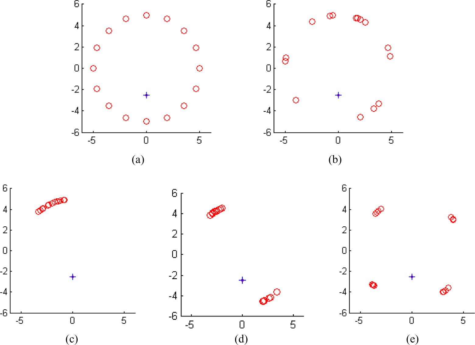
Five different distributions of feature points in simulated experiments. It is simulated in 2D plane that is represented by the x–y coordinates in the plot. The red circles in each plot stand for the landmarks. The blue “+” simulates the position of the camera. (a) First: uniform distribution. (b) Second: random distribution. (c) Third: centralized distribution in one 1/8 arc. (d) Fourth: centralized distribution in two 1/16 arcs. (e) Fifth: centralized distribution in four 1/32 arcs.

While the simulated SLAM is running, the localization error $∊ = | x_{g} - x |$ , which means the distance between ground truth x_g and estimated position x of the camera, is shown in Figure 6. Here, the ground truth is the real position of the camera. Errors of five simulations are compared in Figure 6. Five error curves are separated into two plots in order to analyze conveniently with the error curve of the third simulation. Indexes in legends of plots are the same as indexes of simulations.

Figure 6.

The error curves of the five distributions. The error ε (Y axis) is the function of frame number (X axis). (a) The error curves of the first three distributions. (b) The error curves of the last three distributions.

In Figure 6(a), the first distribution has the least errors as the features are distributed uniformly, while the third distribution performs worse than the former two because of its irregularity. In Figure 6(b), the third distribution still performs worst because the features are so centralized in just one segment that it cannot provide sufficient information for localization. It can be concluded from the error curves that if the landmarks are uniformly distributed, SLAM system will work with less errors. In another words, the more centralized the landmarks are distributed, the worse the accuracy will be. Overall, it is evident that the distribution of feature points has a great impact on the accuracy of SLAM systems.

Feature points selection using FoF

The analysis in the precious section reveals that it will be meaningful if some rules are applied to restrict the distribution of feature points. Thus, it is expected that the locations of feature points can satisfy following conditions: (a) the locations cannot be too converged, (b) the gravity of them should be close to the center of the image, and (c) feature points shouldn’t locate near the edge of the image since great distortion exists in that region. Considering aforementioned analysis, a recent widely used bionic algorithm called FoF³³ is suitable and can be adopted as the restriction. In this chapter, the principle of FoF is stated and then the proposed method using FoF is introduced.

Flocks of features

A biological phenomenon named Flock Behavior ³³ states that the members m_i in the flock $F = {{m_{i}}_{i = 1}^{N_{f}}}$ should be neither too condensed nor too scattered

\begin{array}{l} d_{min} < | m_{i} - m_{j} |, \forall i, j \in {1, 2, ..., N_{f}} \\ d_{max} > | m_{i} - m |, \forall i \in {1, 2, ..., N_{f}} \\ m = m e d i a n (F) o r c e n t r o i d (F) \end{array}

where N_f is the number of members, and m is the center of the flock. d_min is the minimum tolerable distance among the flock, and d_max is the maximum tolerable distance between the center m and other members in the flock.

The well-known Boids algorithm³³ in computer graphics is widely used to simulate flock behaviors. Calling the members of the flock as boids, the flock behavior is maintained by following rules:

Separation: boids try to keep a distance away from other boids.

Cohesion: boids try to fly toward the center of neighbors.

Alignment: boids try to match velocity with near boids.

FoF has been successfully applied in visual tracking especially in tracking articulated objects. Kolsch and Turk³⁴ and Liu et al.²⁸ proposed the FoF tracker in hand tracking using boids and obtained great results. Feature points in hand area is treated as boids and proper feature points can be obtained with the restriction of flock behavior.

Proposed algorithm for feature points selection

Feature points are matched in this frame as the observations to update the state of camera and all the feature points. As the camera has moved, some feature points will be out of view and failed to be matched. If the number of the matched feature points is less than a given threshold minNum, then the FoF selector is employed to add new feature points.

The framework of FoF selector is shown in Figure 7. According to the result of the prediction step, feature points are matched in the current frame. If the number of successfully matched feature points is less than minNum, then a feature selection algorithm is activated to find more feature points. Generally, there will be abundant detected feature points, while just a few of them will be selected as landmarks under the FoF restriction.

Figure 7.

Framework of the FoF selector. FoF: flocks of features.

The core module of the basic FoF selector algorithm is summarized in algorithm 1. All the feature points are treated as boids. The successfully matched features are existing boids and the new detected features are candidate boids. In algorithm 1, W is the weighted map indicating weights of these features, and S_p is the center of all the boids calculated in line 4. For every candidate p in the candidate boids, the positive driving force f_p and negative driving force f_n are computed in algorithm 1 from lines 7 to 14. Here, f_p is the positive driving force pointing from p to the center S_p, driving this point to the center. The negative driving force f_n appears when two boids are too close, acting like the repulsive force between two magnets. For any other boids q, if the distance between the two boids p and q is less than a given threshold d_min, add the repulsive force f(p, q) to f_n. Here, f(p, q) is inversely proportional to the distance between p and q. Finally, the drift of each candidate is obtained as

Δ f = α * f_{p} + β * f_{n}

where α and β are corresponding parameters. If the length of the drift is less than a given threshold T, then the candidate is chosen as the new feature point because boids that drift too much are regarded as “bad” boids in the flock. The new uniformly distributed feature points are gained.

Algorithm 1.

The basic algorithm of FoF Selector.

INPUT: The matched feature points $F_{pre}$ , new detected feature points $F$ , weighted map W

OUTPUT: New feature points $F_{new}$

BEGIN:

$S_{p} \leftarrow \sum_{p \in {F_{pre}, F}} W (p) * p$

$t \leftarrow \sum_{p \in {F_{pre}, F}} W (p)$

for $p \in F$ do

“Perceived center”: $S_{p} \leftarrow \frac{S_{p} - p}{t - W (p)}$

“Positive Driving Force”: $f_{p} \leftarrow S_{p} - p$

“Negative Driving Force”: f_n ← 0

for $q \in F_{pre}$ do

if $p \neq q and | | p - q {| |}_{2} \leq d_{min}$ then

$f_{n} \leftarrow f_{n} + f (p, q)$

end if

end for

if $| | α * f_{p} + β * f_{n} {| |}_{2} < T$ thens

$F_{pre} = {F_{pre}, p}$

end if

end for

$F_{new} \leftarrow F_{pre}$

END

Experiments and discussions

To evaluate the localization accuracy of the proposed feature selection strategy, experiments are conducted in both simulated and real-world environments, which are carried out in indoor environments. The proposed FoF selector is compared with the original random method in the process of feature point selection. Here, the original random method selects the subset of feature points randomly. A single handheld camera is used as the visual sensor moving around and sensing the environment. The camera used in the experiment is a Logitech web camera (see the right part of Figure 1) with 320 × 240 pixels resolution. The original system is run at about one frame per second on a DELL computer with a dual-core processor at 3.1 GHz. Two groups of experiments are conducted. First, a long sequence of 1500 frames is input to SLAM for map building and camera localization, which costs about 25 min. Then, 10 short sequences are used to make a deep analysis.

Experiment on a long sequence

The camera moves around in the lab arbitrarily and captures a long sequence of images. The images are put frame by frame into the SLAM systems using FoF and original random method, respectively. The outputs of the systems are the trajectory of the camera and positions of landmarks.

Figure 8 presents the output of six frames using two different SLAM systems and the corresponding frames are the same for a direct comparison. Feature points are detected and labeled in the left half of each subfigure, and positions of feature points and the trajectory of the camera are drawn in 3-D coordinate systems in the right half. As presented in Figure 8, features are more uniformly distributed in the first and third rows than in the second and fourth rows, which means that the SLAM system using FoF selector performs better than using original random method. Meanwhile, blue circles in the first and third rows are less than in the second and fourth rows in most frames, which indicates feature points are more successfully matched using FoF. In the 3-D coordinate system, presented in the right half of each subfigure, the size of the red ellipse covering the feature point indicates the uncertainty of the estimated position which is in relation to the estimated error covariance. Therefore, it is seen that the red ellipses are smaller in the first and third rows, meaning that 3-D positions of feature points are more accurate and quickly converged using FoF selector.

Figure 8.

Comparison between two SLAM systems. Rows 1 and 3 are results of FoF method and rows 2 and 4 are results of the original random method. On the left half of the output, red and blue circles stand for successfully matched and unmatched features, respectively. On the right, the black curve is the trajectory of the camera and the black triangle indicates camera orientation. Landmarks are represented by red pluses. Surrounding red ellipses mean the uncertainties and red arrows mean that the landmarks are not initialized. SLAM: simultaneous localization and mapping; FoF: flocks of features.

Figure 9 reveals the landmarks and the whole trajectories of the camera output by the SLAM systems with FoF selector and random method, respectively. The red pluses are landmarks of the image and the surrounding red ellipse of each plus represents the error covariance. It is obvious that the landmarks are distributed more uniformly using FoF selector than the random method. Moreover, more landmarks are detected using FoF selector. As a result, errors can be spread uniformly, which restrains the drift to a certain extent.

Figure 9.

The comparison of the landmark distribution using two methods. The red pluses stand for the landmarks. (a) FoF selector and (b) random method. FoF: flocks of features.

Experiments on short sequences

To measure the localization accuracy, 10 short sequences with 100 frames for each sequence are recorded. In addition, motion trajectories of the camera are known to the system. As shown in Figure 10, the camera makes uniform linear motion or uniform circular motion to get the ground truth of the camera trajectories. In our experiments, for each kind of motion, five sequences are made to test the localization accuracy of the SLAM systems.

Figure 10.

Camera movement. The camera moves on a quadrant with radius 0.6m in a constant velocity (left). The camera does the uniform motion for 1 m (right).

Figure 11 shows the results referring to the ground truth using FoF and random method. In each plot, the red dotted curve and the blue curve represent the camera trajectory using FoF and random method, respectively, and the blue dotted curve represents the ground truth. Every trajectory starts from the left end point of the curve and ends on the right end point. In most sequences (e.g. L3, L5, R4, and R5), the estimated trajectories using FoF selector are more close to the ground truth than those using random method, which verifies the better performance in localization accuracy of our approach. However, in some sequences (e.g. L2 and R1), advantages are not distinct because the feature points selected by the random method are also distributed well.

Figure 11.

Camera trajectories of both methods compared to the ground truth. The blue dotted curve is the ground truth of the camera trajectory. The red dotted curve and the blue curve represent the camera trajectory obtained by FoF and random method, respectively. All the curves start from the left end points and end on the right. FoF: flocks of features.

Conclusions

In this article, both theoretical and numerical analyses are made to emphasize the significance of the distribution of feature points in improving the localization accuracy of visual SLAM. According to the analyses, a FoF selector with the flock restriction is introduced to select the feature points when new landmarks need to be added to the map. Experimental results demonstrate that the map is more uniformly distributed and better localization results are obtained when the FoF selector is implemented. In addition, the more feature points are detected, the more effectively FoF selector performs. In future work, novel efficient descriptors will be employed, such as Tree Basis Sparse-coding Inspired Similarity (BASIS),²² Synthetic Basis (SYBA),²⁷ and more sensory data will be combined to improve the localization accuracy for real-world applications, for example, advanced robotics, wearable computing, and augmented reality.

Footnotes

Declaration of conflicting interests

The author(s) declared no potential conflicts of interest with respect to the research, authorship, and/or publication of this article.

Funding

The author(s) received no financial support for the research, authorship, and/or publication of this article.

References

Davison

Reid

Molton

. Monoslam: real-time single camera slam. IEEE Trans Pattern Anal Mach Intell 2007; 29(6): 1052–1067.

Holmes

Klein

Murray

. An o (n²) square root unscented Kalman filter for visual simultaneous localization and mapping. IEEE Trans Pattern Anal Mach Intell 2009; 31(7): 1251–1263.

Roussillon

Gonzalez

Solà

.RT-SLAM: a generic and real-time visual slam implementation. In: Crowley

Draper

and Thonnat. (eds) Computer vision systems. Berlin, Heidelberg: Springer, 2011, pp. 31–40.

Klein

Murray

. Parallel tracking and mapping on a camera phone. In: Science & Technology proceedings, IEEE international symposium on mixed and augmented reality 2009, ISMAR 2009, Orlando, FL, October 2009, pp. 83–86. IEEE.

Kim

J-H

Sukkarieh

. Airborne simultaneous localisation and map building. In: Proceedings of the 2003 IEEE international conference on robotics and automation, ICRA 2003, Taipei, Taiwan, 14–19 September 2003, pp. 406–411.IEEE.

Kim

Sukkarieh

. Autonomous airborne navigation in unknown terrain environments. IEEE Trans Aerosp Electron Syst 2004; 40(3): 1031–1045.

Sáez

Hogue

Escolano

. Underwater 3D SLAM through entropy minimization. In: Proceedings of the 2006 IEEE International Conference on Robotics and Automation, ICRA 2006, Orlando, FL, 15–19 May 2006, pp. 3562–3567. IEEE.

Pizarro

Eustice

Singh

. Large area 3D reconstructions from underwater surveys. In: OCEANS 2004. MTTS/IEEE TECHNO-OCEAN 2004, Kobe, Japan, 9–12 November 2004, Vol. 2, pp. 678–687. IEEE.

Zhaopeng

. A study on monocular simultaneous localization and mapping. PhD Thesis, Institute of Automation, Chinese Academy of Sciences, China, 2011.

10.

Aulinas

Petillot

Salvi

. The slam problem: a survey. In: Proceedings of the 11th international conference of the catalan association for artificial intelligence, CCIA 2008, Sant Martí d’Empúries, Spain, 22–24 October 2008, pp. 363–371. Citeseer.

11.

Chou

Liu

. A robotic indoor 3D mapping system using a 2D laser range finder mounted on a rotating four-bar linkage of a mobile platform. Int J Adv Robot Syst 2013; 10(1): 257–271.

12.

Bethencourt

Jaulin

. 3D reconstruction using interval methods on the kinect device coupled with an IMU. Int J Adv Robot Syst 2013; 10(2): 323–330.

13.

Müller

Weber

Wermter

. Ratslam on humanoids-a bio-inspired slam model adapted to a humanoid robot. In: International conference on artificial neural networks (eds, Wermter

Weber

Duch

), Hamburg, Germany, 15–19 September 2014, pp. 789–796. Switzerland: Springer.

14.

Kostavelis

Boukas

Nalpantidis

. Stereo-based visual odometry for autonomous robot navigation. Int J Adv Robot Syst 2016; 13: 1–21.

15.

Thrun

Burgard

Fox

. Probabilistic robotics. Cambridge: MIT press, 2005.

16.

Solà

Vidal-Calleja

Civera

. Impact of landmark parametrization on monocular EKF-SLAM with points and lines. Int J Comput Vis 2012; 97(3): 339–368.

17.

Moore

Stouch

. A generalized extended Kalman filter implementation for the robot operating system. In: IAS 2014 – The 13th international conference on intelligent autonomous systems (eds, Menegatti

Michael

Berns

), Centro Congressi Padova, Padova, Italy, 15–19 July 2014, pp. 335–348. Springer.

18.

Roller

Montemerlo

Thrun

. Fastslam 2.0: an improved particle filtering algorithm for simultaneous localization and mapping that provably converges. In: Proceedings of the international joint conference on artificial intelligence (IJCAI-03) (eds Gottlob

Walsh

), Acapulco, Mexico, 9–15 August 2003, pp. 1151–1156.

19.

Thrun

Liu

Koller

. Simultaneous localization and mapping with sparse extended information filters. Int J Robot Res 2004; 23(7–8): 693–716.

20.

Burgard

Fox

Jans

. Sonar-based mapping with mobile robots using EM. In: Machine learning, 1999, pp. 67–76. Morgan Kaufmann Publishers, inc.

21.

Sola

Vidal-Calleja

Civera

. Impact of landmark parametrization on monocular EKF-SLAM with points and lines. Int J Comput Vis 2012; 97(3): 339–368.

22.

Fowers

Desai

Lee

. Efficient tree-based feature descriptor and matching algorithm. J Aerosp Inf Syst 2014; 11(9): 596–606.

23.

Shi

Tomasi

. Good features to track. In: 1994 IEEE computer society conference on computer vision and pattern recognition, proceedings, Seattle, Washington, 21–23 June 1994, pp. 593–600. IEEE.

24.

Rosten

Porter

Drummond

. Faster and better: a machine learning approach to corner detection. IEEE Trans Pattern Anal Mach Intell 2010; 32(1): 105–119.

25.

Lowe

Little

. Mobile robot localization and mapping with uncertainty using scale-invariant visual landmarks. Int J Robot Res 2002; 21(8): 735–758.

26.

Murillo

Guerrero

JJ,

Sagüés

. Surf features for efficient robot localization with omnidirectional images. In: IEEE international conference on robotics and automation, ICRA 2007, Roma, Italy, 10–14 April 2007, pp. 3901–3907. IEEE.

27.

Desai

Lee

. Visual odometry drift reduction using SYBA descriptor and feature transformation. IEEE Trans Intell Transp Syst 2016; 17: 1–13.

28.

Liu

Cui

Ding

. Robust hand tracking with Hough forest and multi-cue flocks of features. In: Fowlkes

Wang

Choi

M-H

. (eds) Advances in visual computing. Berlin, Heidelberg: Springer, 2012, pp. 458–467.

29.

Smith

Cheeseman

. On the representation and estimation of spatial uncertainty. Int J Robot Res 1986; 5(4): 56–68.

30.

Civera

Davison

AJ,

Martinez Montiel

. Inverse depth parametrization for monocular slam. IEEE Trans Robot 2008; 24(5): 932–945.

31.

Hartley

Zisserman

. Multiple view geometry in computer vision. Cambridge: Cambridge University Press, 2003.

32.

Zhang

. Computer visionął computational theories and algorithm. Beijing: The Science Press of China, 1998.

33.

Reynolds

. Flocks, herds and schools: a distributed behavioral model. ACM Siggraph Comput Graph 1987; 21(4): 25–34.

34.

Kölsch

Turk

. Fast 2D hand tracking with flocks of features and multi-cue integration. In: IEEE computer society conference on computer vision and pattern recognition (CVPR 2004), Washington, DC, 27 June–2 July 2004, pp. 158–158. IEEE.

Feature points selection with flocks of features constraint for visual simultaneous localization and mapping

Abstract

Keywords

Introduction

Framework of EKF-based visual SLAM

Overview of visual SLAM

The EKF

Analysis of the distribution of feature points

Theoretical analysis

Numerical analysis

Feature points selection using FoF

Flocks of features

Proposed algorithm for feature points selection

Experiments and discussions

Experiment on a long sequence

Experiments on short sequences

Conclusions

Footnotes

Declaration of conflicting interests

Funding

References