Avoiding blind leading the blind

Abstract

Virtual pheromone trailing has successfully been demonstrated for navigation of multiple robots to achieve a collective goal. Many previous works use a pheromone deposition scheme that assumes perfect localization of the robot, in which, robots precisely know their location in the map. Therefore, pheromones are always assumed to be deposited at the desired place. However, it is difficult to achieve perfect localization of the robot due to errors in encoders and sensors attached to the robot and the dynamics of the environment in which the robot operates. In real-world scenarios, there is always some uncertainty associated in estimating the pose (i.e. position and orientation) of the mobile service robot. Failing to model this uncertainty would result in service robots depositing pheromones at wrong places. A leading robot in the multi-robot system might completely fail to localize itself in the environment and be lost. Other robots trailing its pheromones will end up being in entirely wrong areas of the map. This results in a “blind leading the blind” scenario that reduces the efficiency of the multi-robot system. We propose a pheromone deposition algorithm, which models the uncertainty of the robot’s pose. We demonstrate, through experiments in both simulated and real environments, that modeling the uncertainty in pheromone deposition is crucial, and that the proposed algorithm can model the uncertainty well.

Introduction

To set the scene for this article, consider the following example:

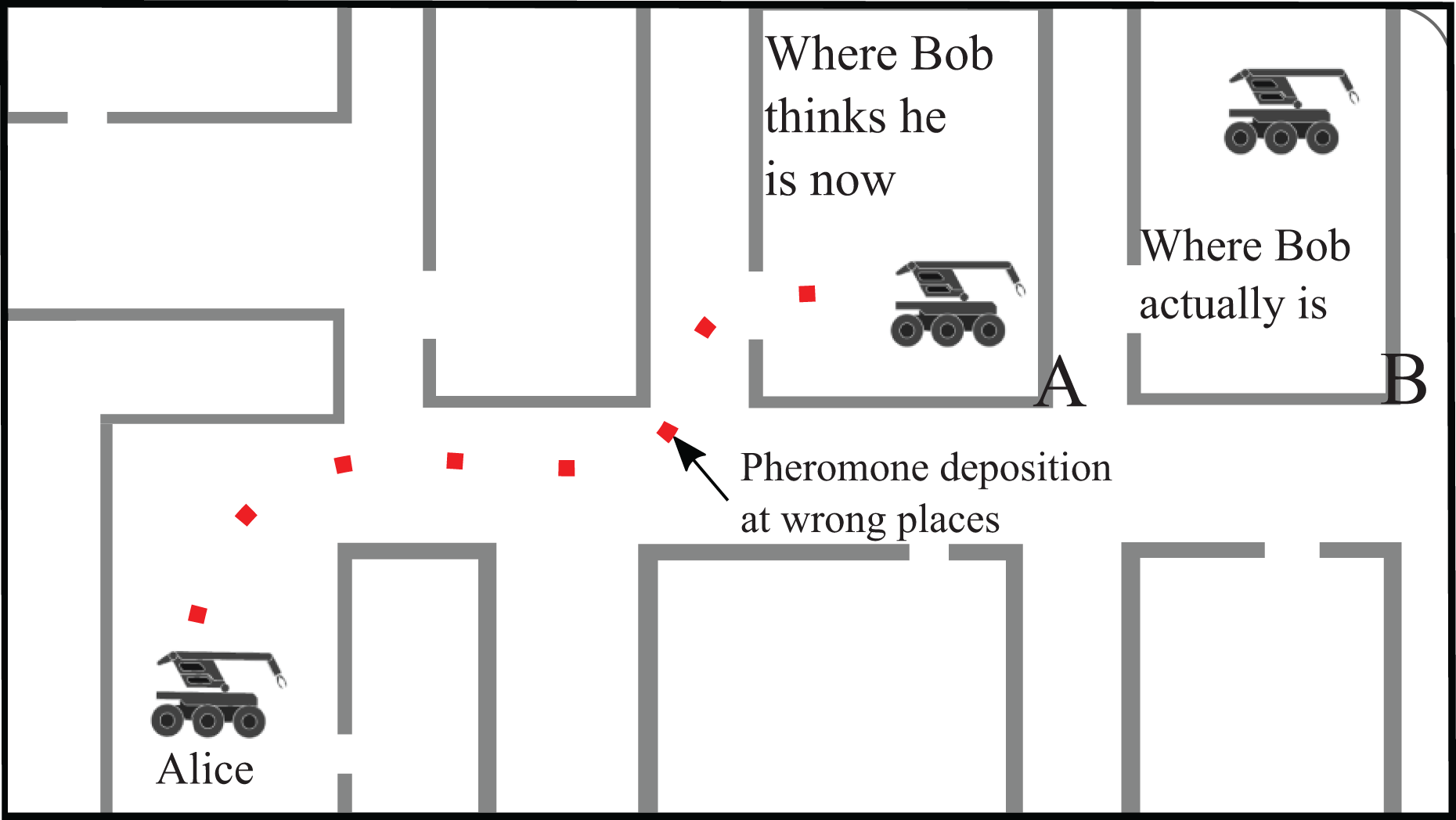
There is a multi-robot system employing pheromone trailing mechanism. Bob is the leader robot and Alice follows the pheromone trails left by Bob, as shown in Figure 1. They are both on a rescue mission at a disaster site to find a victim and provide medical aid. They are both given the approximate map of the site. Bob uses one of the traditional pheromone deposition schemes to deposit pheromones and Alice follows sensing the trail, as shown in Figure 1. Both the robots (leader Bob and follower Alice) have localization and mapping units along with sensors attached to them. The robots associate and match the registered features of the map with the features extracted from the sensor data in order to estimate their position in the map. If the estimation is good, then there is less error between the estimated and the true position of the robot. If the estimation is bad, the estimated position is far from the robots true position. The robots deposit the pheromones at their estimated position. Hence, in case of good estimation (and hence localization), pheromones are deposited at nearly the correct place. But, in case of bad estimation, the pheromones are deposited at wrongly estimated positions in the map. This difference in true and estimated position may arise due to many similar features in the map, noisy environment, noisy sensors, wheel slip, lack of good features, and others. Pheromone deposition at wrong places is further explained in Figure 2, in which robot’s estimated position is Pos.E at coordinates X = 15 and Y = 10. Robot’s true position is Pos.T at coordinates X = 25 and Y = 10. Hence, the pheromones are wrongly deposited by the robot at Pos.E (X = 15 and Y = 10).

Figure 1.

Bob’s localization failure results in its pheromone deposition at wrong places. Like Bob, the pheromone trailing Alice too will end up in the wrong place.

Figure 2.

Pheromone deposition at wrong places. Robots deposit pheromones at their estimated positions which might differ from their true position. In this example, Robot’s estimated position is Pos.E at coordinates X = 15 and Y = 10. Robot’s true position is Pos.T. at coordinates X = 25 and Y = 10. Hence, the pheromones are wrongly deposited at Pos.E (X = 15 and Y = 10).

As shown in Figure 1, Bob gets lost as there are many similar features in the environment, and the disaster site is cluttered with noise. Bob “estimates” that it is at location A. However, Bob’s true position is B. But, since Bob does not model its positional uncertainty in depositing pheromones, it keeps depositing pheromones according to its estimated position in the map, which differs from its true position. Therefore, the pheromones deposited by Bob end up at wrong places as well. In Figure 1, pheromones deposited at Bob’s wrongly estimated position are shown in red color.

Alice, the trail following robot must catch up with Bob to provide assistance and follows the Bob’s pheromone trails. Alice, which relies on pheromone trails, finds the same amount of pheromones deposited by Bob everywhere and blindly keeps following the trails deposited at Bob’s wrongly estimated positions. Eventually, Alice ends up at the wrong position A as shown in Figure 1 and does not find Bob which is truly located at position B. Alice too leaves its own pheromone trails for other robots. Irrespective of whether Alice’s localization was good or not, Alice actually goes to position A following the Bob’s trails, and hence, all the robots end up at wrong places of the map.

This is a classical example of “blind leading the blind” case. The fault does not lie with Bob, or Bob’s localization unit as good localization is difficult to achieve in cluttered environments. The real culprit is Bob’s pheromone deposition module which does not model the Bob’s positional uncertainty while depositing pheromones. Therefore, Alice and other robots have no clue if Bob was lost at some place in the map.

Only if Alice had some clue that Bob was actually lost at some place in the map, it would have been in a position to decide if it should follow the trails or explore the environment on its own based on other conditional factors.

Problem statement

In the absence of modeling the positional uncertainty in pheromone deposition, pheromones will be deposited at the wrong places in the map. Other robots trailing the pheromones as well may end up in wrong areas of map which will reduce the efficiency of the multi-robot system.

Main idea of this article

Pheromone deposition and positional uncertainty are (and must be) integrated and modeled together. As shown in Figure 3, if Bob’s localization module estimates a large uncertainty in its current position in the map, Bob deposits less pheromones and disperses them across its current position. The amount of pheromones deposited is inversely proportional to the estimated positional uncertainty. If the robot has localized itself well in the map, large amount of pheromones are deposited confidently in a small area centered around the current position. This enables Alice to decide if it should follow the leader robot. If the trails are dispersed and weak, the follower robot may decide not to follow the “lost” leader robot and instead explore the map on its own.

Figure 3.

Bob reduces pheromone deposition and disperses them depending on its uncertainty. Trailing Alice now has some idea that Bob was lost at point P and is in a better position to take decision.

New contributions of this article

We propose pheromone deposition with uncertainty modeling. Pheromone deposition scheme, which can be integrated with estimation filters (like extended Kalman filter (EKF) and particle filter (PF)), is proposed. More pheromones are deposited at locations where the robot’s localization is comparatively better, and vice versa. The pheromones are deposited as a gradient in the map, which allow the robots to move toward the direction with maximum rate of change of pheromones. A pheromone evaporation considering the influence of ambient pheromones is also presented. The proposed method is tested in both simulation and real environment. Speed adaption by trailing robots with reference to the pheromones sensed is presented as a practical application.

Related works

The induction of virtual pheromone trailing in robotics is not new and there is a plethora of works dealing with using this idea to achieve a complex task for multi-robot cooperation in the literature. The idea is inspired from biology and nature. Many insects (e.g. ants, bees, and wasps) deposit particular chemicals called as “pheromones” ¹ in order to attract other members of the same species. Sometimes they are also used to warn other species, or claim territory. With regard to robotics and pheromone trailing, an extensive review has been carried out in the works found in the literatures. ^{2 –4}

Regarding comparison with other works, we find it suffice to mention that the proposed work is one of the first work in the literature to model the positional uncertainty of the robot in the map, to the best of our survey. Ravankar et al. mentioned this idea in their work, ⁵ but their work mainly focused on combining pheromones and anti-pheromones ^6,7 in a single framework with no experimental verification and constant pheromone deposition only at certain points of the map. We extended the work by mathematically describing the deposition of pheromones anywhere in the map. We also extended the work by concretely integrating the evaporation mechanism of the pheromones while also considering the effect of ambient pheromones. Moreover, a thorough test in both simulation and real environment with integration in simultaneous localization and mapping (SLAM) has been provided in this work. Other than the works of Ravankar et al., most of the previous works consider a perfect localization model of the robot. Previous works on pheromone signalling in robotics have been mainly concentrated to mimic the swarm behavior using attractive pheromones. ⁸ The applications included process control, ^9,10 communication, ^11,12 and to mimic swarm behavior. ¹³ Works by Calvo et al. and Doi ^14,15 have focused on applications of robot surveillance. An interesting work of using virtual pheromones with multi-robots is presented in the studies by Pearce et al. (2003, 2006) ^6,16 to test the dispersive behavior of multi-robots.

The proposed work does not deals with any sort of optimization techniques, which involves pheromones (e.g. ant colony optimization like in the study by Sundareswaran et al. ¹⁷ ). On the contrary, we took an entirely fresh approach to deal with the problem of depositing pheromones in the map at a more fundamental level by also modeling the positional uncertainty of the robot.

A brief introduction to robot state and uncertainty estimation using various filters

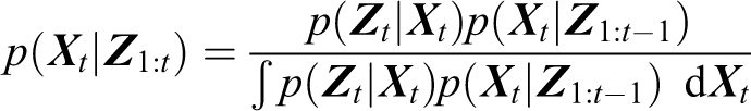
An autonomous mobile robot in an unknown environment needs to build a map of its surrounding, while simultaneously updating its position in the map, also known as the SLAM problem. If a map is available, the robot must localize itself in the map by associating features (e.g. lines, corners, or color) in the map and the features extracted from the sensors attached to the robot to estimate its position. It is a challenging problem due to the uncertainties associated with sensors, robot motion, and dynamics of the environment. Probabilistic filters have been successfully employed to mathematically model this uncertainty by representing ambiguity and degree of belief using the calculus of probability.

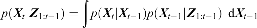
The most general algorithm for calculating the probabilistic beliefs is given by the Bayes filter. The state of the robot (x_t) at time t is indicated by a vector comprising of its pose [x y] ^T and orientation (θ) as, $x_t={\left[x y \theta \right]}^T$ . Bayes filter is a recursive filter in which the belief bel(x_t) at time t is calculated from the prior belief bel(x_t−1) at time t − 1. Given a control u_t at time t, Bayes filter calculates the predictive belief bel(x_t) just before the observation (z_t) using its prior belief (bel(x_t)) as

$\begin{array}{l}\overline{\text{bel}\left(x_t\right)}=\int p\left(x_t\right)|u_t,x_{t-1} \text{bel}\left(x_{t-1}\right) \text{d}{x}_{t-1}\hfill \end{array}$

1

This is known as the prediction step. The next step is that of correction in which the predicted belief $(\overline{\text{bel}\left(x_t\right)})$ is multiplied with the probability that the measurement z_t may have been observed. Since the probability density function may not integrate to 1, the result is normalized by the normalization constant η

$\begin{array}{l}\text{bel}\left(x_t\right)=\eta p\left(z_t\right)|x_t \overline{\text{bel}\left(x_t\right)}\hfill \end{array}$

2

There are many variants of Bayes filter, which can estimate the state of the robot and the uncertainty associated with this estimate. Although a detailed explanation of these filters is out of the scope of this article, what is most relevant to this article is that all these filters can estimate the state and the associated uncertainty, which will be used to deposit pheromones by the robots. A brief discussion of these filters is presented here with pointers for detailed explanation. Moreover, we limit our discussion to three most widely used filters: EKF, unscented Kalman filter (UKF), and PF.

Extended Kalman filter

EKF is a powerful mathematical tool to model the uncertainties of the sensors attached to the robot and has been demonstrated successfully with laser range sensors, vision sensors, inertial sensors, and so on for mapping and localization. The standard Kalman filter assumes linear state and measurement transitions with Gaussian noise. An EKF overcomes the nonlinearity by employing Jacobians and (first order) Taylor expansion in the nonlinear model. The belief at time t is represented by the mean μ_t and the covariance matrix Σ _t . We have two nonlinear functions: the state transition function g(⋅) and the measurement transition function h(⋅), given as

$\begin{array}{l}{x}_t=g\left(u_t,x_{t-1}\right)+{\epsilon }_t\hfill \\ z_t=h\left(x_t\right)+{\delta }_t\hfill \end{array}$

3

where ε_t, and δ_t are the noises. The nonlinear function g(⋅) is approximated by the value at μ_t−1 and control u_t through a Taylor expansion

$\begin{array}{ll}g\left(u_t,x_{t-1}\right)\hfill & \approx g\left(u_t,{\mu }_{t-1}\right)+g\prime \left(u_t,{\mu }_{t-1}\right)\left(x_{t-1}-{\mu }_{t-1}\right)\hfill \\ \hfill & =g\left(u_t,{\mu }_{t-1}\right)+G_t\left(x_{t-1}-{\mu }_{t-1}\right)\hfill \end{array}$

4

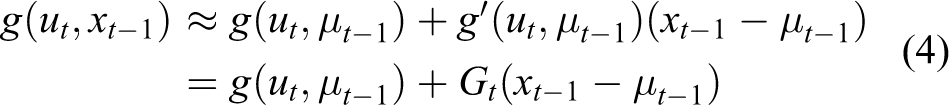
where G_t is the Jacobian given as the first derivative of g at μ_t−1. EKF implements the same linearization for measurement function h at the predicted mean $\overline{{\mu }_t}$

$\begin{array}{ll}h\left(x_t\right)\hfill & \approx h\left(\overline{{\mu }_t}\right)+h\prime \left(\overline{{\mu }_t}\right)\left(x_t-\overline{{\mu }_t}\right)\hfill \\ \hfill & =h\left(\overline{{\mu }_t}\right)+H_t\left(x_t-\overline{{\mu }_t}\right)\hfill \end{array}$

5

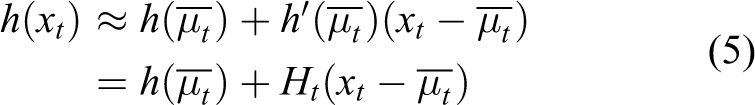
where H_t is the Jacobian given as the first derivative of g at $\overline{{\mu }_t}$ . The details about the prediction and correction steps of EKF can be found in literatures. ^{18 –21}

Unscented Kalman filter

Unlike EKF, which uses Taylor series expansion to linearize the transformation of a Gaussian, an UKF performs a stochastic linearization through statistical linear regression process. The main idea behind UKF is that it is easier to approximate the probability function than the nonlinear function. For an n-dimensional Gaussian with mean μ and covariance Σ, UKF extracts 2n + 1 points (also called sigma points χ^[i]) from the Gaussian and passes these through g. The sigma points are chosen according to the following rules

$\begin{array}{ll}{\chi }^{[0]}\hfill & =\mu \hfill \\ {\chi }^{[i]}\hfill & =\mu +{\left(\sqrt{(n+\lambda )\Sigma }\right)}_i \text{for} i=1,\cdots ,n\hfill \\ {\chi }^{[i]}\hfill & =\mu -{\left(\sqrt{(n+\lambda )\Sigma }\right)}_{i-n} \text{for} i=n+1,\cdots \mathrm{,2}n\hfill \\ \hfill & \hfill \end{array}$

6

where $\lambda ={\alpha }^2\left(n+\kappa \right)-n$ and α and κ are scaling parameters that determine how far the sigma points are spread from the mean. Each sigma point χ^[i] has two associated weights: $w_m^{[i]}$ used when computing the mean, and $w_c^{[i]}$ used when computing the covariance. The sigma points are then passed through the nonlinear function g

$\begin{array}{l}{Y}^{[i]}=g\left({\chi }^{[i]}\right)\hfill \end{array}$

7

Parameters μ and Σ of the resulting Gaussian are extracted from the mapped sigma points Y^[i] according to the following equation

$\begin{array}{ll}\mu \hfill & =\sum _{i=0}^{2n}{w}_m^{\left[i\right]}{Y}^{\left[i\right]}\hfill \\ \Sigma \hfill & =\sum _{i=0}^{2n}{w}_c^{\left[i\right]}\left(Y^{[i]}-\mu \prime \right){\left(Y^{[i]}-\mu \prime \right)}^T\hfill \\ \hfill & \hfill \end{array}$

8

A detailed explanation of UKF can be found in the literatures. ^{18 –23}

Particle filter

PF is a nonlinear state estimator based on Bayesian filtering. It is a sequential Monte Carlo-based technique, which models the probability density using a set of discrete points. PF can represent a much broader space of distributions than, for example, Gaussians. Generally, robot localization involves the estimating the state X _t of the robot, where ${\mathit{X}}_t={\left[x,y,\theta \right]}^T$ with measurements Z _t at time t. The state space and observation equations are given in the equation

${\mathit{X}}_t={\mathit{f}}_t\left({\mathit{X}}_{t-1},{\mathit{u}}_t\right)\left(\text{state}\hspace{0.17em}\text{equation}\right)$

${\mathit{Z}}_t={\mathit{h}}_t\left({\mathit{X}}_t,{\mathit{v}}_t\right)\hspace{1em}\hspace{1em}\text{(observation}\hspace{0.17em}\text{equation)}$

where X _t is a state vector with noise u _t and Z _t is a set of observations with noise v _t . f _t (⋅) is a nonlinear system transition function and g _t (⋅) is a nonlinear measurement function. By Bayes’ formula, the posterior state distribution $p\left({\mathit{X}}_t|{\mathit{Z}}_{1:t-1}\right)$ is given as

$p\left({\mathit{X}}_t|{\mathit{Z}}_{1:t-1}\right)=\int p\left({\mathit{X}}_t|{\mathit{X}}_{t-1}\right)p\left({\mathit{X}}_{t-1}|{\mathit{Z}}_{1:t-1}\right) \text{d}{\mathit{X}}_{t-1}$

$p\left({\mathit{X}}_t|{\mathit{Z}}_{1:t}\right)=\frac{p\left({\mathit{Z}}_t|{\mathit{X}}_t\right)p\left({\mathit{X}}_t|{\mathit{Z}}_{1:t-1}\right)}{\int p\left({\mathit{Z}}_t|{\mathit{X}}_t\right)p\left({\mathit{X}}_t|{\mathit{Z}}_{1:t-1}\right) \text{d}{\mathit{X}}_t}$

Particles or samples of posterior distribution are represented as

${\mathit{X}}_t=X_t^{[1]},X_t^{[2]},X_t^{[2]},\cdots ,X_t^{[M]}$

where M denotes the total number of particles in the particle set X _t . Each particle $X_t^{[m]}$ $\left(1\le m\le M\right)$ is a concrete instantiation of the state at time t and has a weight $w_t^m$ associated with it. X_t approximates the distribution p(X) by

$p\left(X\right)\approx \sum _{m=1}^M{w}^{\left[m\right]}\delta \left(X-X^{[m]}\right)$

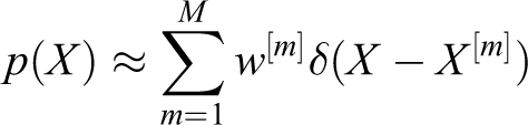
where δ(⋅) is the Dirac delta function. Initially, we generate M particles from the distribution p(X) and each particle is assigned a uniform weight equal to $\frac{1}{M}$ . PF approximates the state by drawing a set of M weighted random samples from the importance density function π(⋅). The normalized importance weight ${\overline{w}}_t^{\left[m\right]}$ and updated weight $w_t^{\left[m\right]}$ , which governs the resampling is given by

${\overline{w}}_t^{[m]}=\frac{p\left(X\right)}{\pi \left(X\right)}=\frac{w_t^{\left[m\right]}}{\sum _{m=1}^M{w}_t^{\left[m\right]}}$

$w_t^{[m]}\propto \frac{p\left(Z_t|X_t^{\left[m\right]}\right)p\left(X_t^{\left[m\right]}|X_{t-1}^{\left[m\right]}\right)}{\pi \left(X_t^{\left[m\right]}|X_{0:t-1}^{\left[m\right]},Z_{0:t}\right)}{w}_{t-1}^{\left[m\right]}$

A detailed explanation of PF can be found in the literatures. ^{19,20,24 –26}

Apart from the abovementioned filters, there are many other filters like histogram filter, information filter, and others which have been explained in detail in the literatures. ^{19 –21} All of these filters can estimate the state of the robot and the uncertainty associated with the estimate. Readers may find a comparison of the merits and limitations of various filters in the study by Kurt-Yavuz and Yavuz. ²⁷

Pheromone deposition with uncertainty modeling

Irrespective of the filter used, it is assumed that the state [x y θ] ^T of the robot is estimated along with the uncertainty associated. We first discuss the pheromone deposition in the map in section “Pheromone deposition.” Later, the pheromone evaporation mechanism is explained in section “Pheromone evaporation.”

Pheromone deposition

The robot’s uncertainty in state is generally represented by the covariance matrix (Σ_t)

${\Sigma }_t=\left[\begin{array}{lll}{\sigma }_x^2\hfill & {\sigma }_{xy}\hfill & {\sigma }_{x\theta }\hfill \\ {\sigma }_x^2\hfill & {\sigma }_y^2\hfill & {\sigma }_{y\theta }\hfill \\ {\sigma }_{x\theta }\hfill & {\sigma }_{y\theta }\hfill & {\sigma }_{\theta }^2\hfill \end{array}\right]$

9

If the uncertainty in robot’s pose given by Σ_t is large, the robot should deposit less pheromones, and vice versa. Hence, the pheromone deposition can be modeled as

$\text{Amount}\hspace{0.17em}\text{of}\hspace{0.17em}\text{phermones}\propto \frac{1}{\text{Uncertainty}\hspace{0.17em}\text{given}\hspace{0.17em}\text{by}\hspace{0.17em}{\Sigma }_t}$

10

Σ_t also contains the uncertainty in the orientation (θ). However, the amount of pheromones deposited in the map are scalar in nature. The robot can deposit the same number of pheromones at the same spatial position with any orientation (correct or not) at that position. Hence, a sub-matrix (Σ_xy) of covariance Σ_t is considered without the orientation uncertainty, and the pheromone deposition is modeled as

$\begin{array}{l}{\Sigma }_{xy}=\left[\begin{array}{cc}{\sigma }_x^2& {\sigma }_{xy}\\ {\sigma }_{xy}& {\sigma }_y^2\end{array}\right]\\ \text{Amount}\hspace{0.17em}\text{of}\hspace{0.17em}\text{phermones}\propto \gamma \propto \frac{1}{\text{Uncertainty}\hspace{0.17em}\text{given}\hspace{0.17em}\text{by}\hspace{0.17em}{\Sigma }_{xy}}\end{array}$

11

Here, γ is a factor which controls the amount of pheromones to be deposited.

The eigenvalues $\left({\lambda }_1,\cdots {\lambda }_n\right)$ and eigenvectors $\left({\overrightarrow{v}}_1,\cdots {\overrightarrow{v}}_n\right)$ of the matrix Σ_xy denotes the magnitude and direction of the variance, respectively.

The main idea is to deposit pheromones inversely proportional to the uncertainty given by the covariance matrix. The pheromone controller factor γ is thus inversely proportional to the product of eigenvalues of the covariance matrix

$\begin{array}{l}\gamma \propto \frac{1}{\prod _{i=1}^n{\lambda }_i},\to \gamma =\tau \cdot \frac{1}{\prod _{i=1}^n{\lambda }_i}\hfill \end{array}$

12

and τ is a constant determined experimentally.

Other robots can also deposit pheromones on the top of already existing pheromones at any position in the map. The range of the sensor employed is denoted by z_rng. Pheromone deposition at a location is defined as the function

$\begin{array}{l}{P}_{\text{loc}}=f\left(x,y\right)\hfill \end{array}$

13

Here, x and y represents the spatial coordinates of the robot’s estimated position in the map. In the present work, we discuss the case of wheeled mobile robots and their motion in two-dimensional space. The number of pheromones deposited at a certain location decays exponentially with distance from the robot’s position, and the deposition is modeled as

$P_{\text{loc}}=\{\begin{array}{cc}\gamma \cdot e^{-\left(\frac{x^2}{{\lambda }_1^2}+\frac{y^2}{{\lambda }_2^2}\right)}& \text{within}\hspace{0.17em}{z}_{rng}\\ 0& \text{otherwise}\end{array}$

14

Pheromones are deposited only within the range of the sensor (z_rng). P_loc is a scalar field which associates amount of pheromones with the spatial location in the map. The gradient of this function generates a vector field, which indicates the direction in which there is the largest increase in pheromones, and also the magnitude of those vectors in the vector field to the robot

$\begin{array}{l}\nabla P=\frac{\partial P_{\text{loc}}}{\partial x}\widehat{i}+\frac{\partial P_{\text{loc}}}{\partial y}\widehat{j}\hfill \end{array}$

15

where, $\widehat{i},\widehat{j}$ are standard unit vectors. Substituting P_loc, we get

$\begin{array}{l}\nabla P=\frac{\partial }{\partial x}\gamma \cdot e^{-\left(\frac{x^2}{{\lambda }_1^2}+\frac{y^2}{{\lambda }_2^2}\right)}\widehat{i}+\frac{\partial }{\partial y}\gamma \cdot e^{-\left(\frac{x^2}{{\lambda }_1^2}+\frac{y^2}{{\lambda }_2^2}\right)}\widehat{j}\\ =-\frac{2x\gamma }{{\lambda }_1^2}\cdot e^{-\left(\frac{x^2}{{\lambda }_1^2}+\frac{y^2}{{\lambda }_2^2}\right)}\widehat{i}-\frac{2y\gamma }{{\lambda }_1^2}\cdot e^{-\left(\frac{x^2}{{\lambda }_1^2}+\frac{y^2}{{\lambda }_2^2}\right)}\widehat{j}\\ =-2\gamma \cdot e^{-\left(\frac{x^2}{{\lambda }_1^2}+\frac{y^2}{{\lambda }_2^2}\right)}\cdot \left[\frac{x}{{\lambda }_1^2} \frac{y}{{\lambda }_2^2}\right]\times {[\widehat{i} \widehat{j}]}^T\end{array}$

16

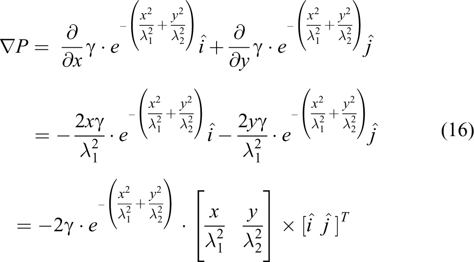
As compared to a scalar representation of the pheromones in the map, the gradient vector field provides more information to the robots in pheromone trailing. For large area pheromone depositions, the gradient points the robot in the direction of the maximum rate of increase of the pheromones, and its magnitude is the slope of the graph in that direction, which enables the robot to properly track the pheromones. Moreover, the deposition is probabilistic and if the localization of the robot is good, more pheromones are deposited. However, if the robot fails to localize itself, less or no pheromones are deposited. The entire pheromone deposition scheme is shown in the flowchart in Figure 4.

Figure 4.

Flowchart.

Multiple robots may deposit pheromones at the same or nearby locations and the two pheromone fields gets merged by equation (16). This is represented in Figure 5, which shows the additive pheromones resulting from deposition in the vicinity.

Figure 5.

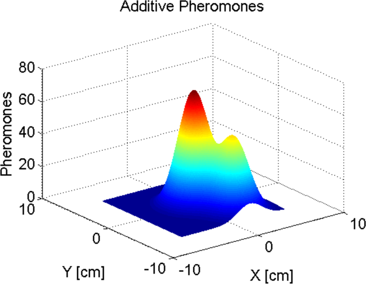
Addition of pheromone fields in vicinity.

Pheromone evaporation

Like in nature, the pheromones are modeled to evaporate with time. The rate of evaporation of pheromones is proportional to the difference in the pheromones deposited (P) and that of the ambient or nearby pheromones (P_a). In other words, pheromones deposited at a lonely location with no nearby (i.e. within the sensor range z_rng) pheromones evaporate faster. If the robot(s) deposit large number of pheromones around an area, it is an indication of a trail toward a source (e.g. food) and the presence of ambient pheromones slowdown the evaporation process. The rate of evaporation of pheromones is given by

$\frac{\text{d}P}{\text{d}t}=-K\cdot \left(P-P_a\right)$

17

where K is a constant. Equation (17) is a separable differential equation. Integrating this equation, we get

$\begin{array}{l}\int \frac{1}{\left(P-P_a\right)}\text{d}P=\int -K\text{d}t\\ \Rightarrow \ln \left|P-P_a\right|=-Kt+c\\ \Rightarrow \left|P-P_a\right|=e^{-Kt+c}\\ \Rightarrow \left|P-P_a\right|=e^{-Kt}\cdot e^c\\ \Rightarrow \left|P-P_a\right|=C\cdot e^{-Kt}\end{array}$

18

which gives

$\Rightarrow P\left(t\right)=C\cdot e^{-Kt}+P_a$

19

which is a general solution of the differential equation, and C is a constant. The constant K is a controlling factor, which governs the rate of evaporation of the pheromones in the map. The factors K and C are determined by the boundary conditions. At t = 0, when there are P₀ pheromones, from equation (19)

$\begin{array}{l}P\left(t=0\right)=P_0=C+P_a\\ \Rightarrow C=P_0-P_a\end{array}$

20

At time t_m > 0, the pheromones $\left(P_{t_{tm}}\right)$ are given from equation (19) as

$\begin{array}{l}P\left(t=t_m\right)=P_{t_{tm}}=C\cdot e^{-K{t}_m}+P_a\hfill \end{array}$

21

Substituting the constant C given by equation (20) into the above equation

$\begin{array}{l}{P}_{t_{tm}}=\left(P_0-P_a\right)\cdot e^{-K{t}_m}+P_a\hfill \end{array}$

22

solving which we get the expression for the constant K as

$K=-\frac{1}{t_m}\ln \left(\frac{P_{t_{tm}}-P_a}{P_0-P_a}\right)$

23

We fix a threshold for the amount of pheromones deposited at a location and sensed by the robot below which the robot “rejects” the trail. If a following robot comes across a very weak trail, it does not follow it and rather carries its own exploration. If P₀ is the total pheromone count in the beginning, we set this threshold to δP₀, where 0 < δ ≤ 1. For maximum amount of pheromones deposited at a location, the total time it takes for the pheromone to evaporate to the threshold value δP₀ is calculated. From equation (22)

$\begin{array}{l}\delta \cdot P_0=\left(P_0-P_a\right)\cdot e^{-Kt}+P_a\mathrm{.}\hfill \end{array}$

24

Substituting the value of K from equation (23) into the above equation

$\begin{array}{ll} \hfill & \delta P_0=\left(P_0-P_a\right)\cdot e^{\frac{t}{t_m}\ln \left(\frac{P_{t_{tm}}-P_a}{P_0-P_a}\right)}+P_a\hfill \\ \hfill & \Rightarrow \ln \left(\frac{\delta P_0-P_a}{P_0-P_a}\right)=\frac{t}{t_m}\ln \left(\frac{P_{t_{tm}}-P_a}{P_0-P_a}\right)\hfill \end{array}$

25

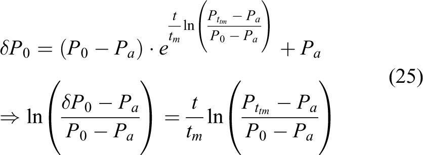
Solving

$t=t_m\frac{\ln \left(\frac{\delta P_0-P_a}{P_0-P_a}\right)}{\ln \left(\frac{P_{t_{tm}}-P_a}{P_0-P_a}\right)}$

26

While modeling the system, equation (26) is useful in calculating the total time it takes for the pheromones to evaporate below a threshold level considering the size of the area and the speed of the robot. The parameter δ tunes the rate of evaporation according to these characteristics of the environment and the robot.

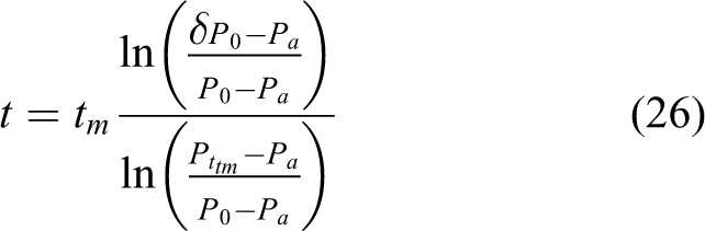
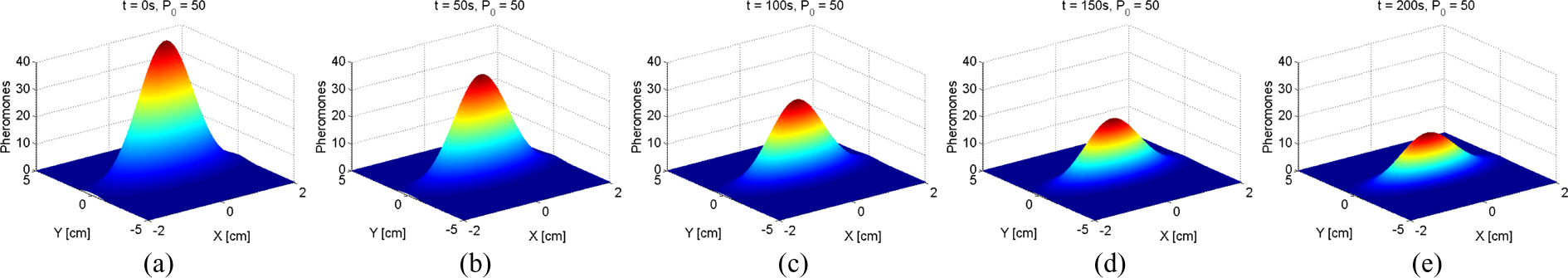
Figure 6 shows the evaporation of pheromones with time when the robot deposits a large value of pheromones (P₀ = 50) with no ambient pheromones (P_a = 0). The value of parameter K is determined so that pheromones evaporate to a threshold value of 18 in around 300 s or 5 min (i.e. P_t=300 = 18). At the same rate, Figure 7 shows the evaporation of pheromones with initially P₀ = 35 amount of pheromones deposited. It takes about 116 s for the pheromones to evaporate to the threshold value. This value is chosen considering the speed of the robots and the characteristics of the environment. Typically, in indoor environments a speed of 0.5 m/s is safe for the mobile robots. Considering the other factors like the dynamics of the environment, smoothness of the surface, and so on. Equations (19), (23), and (26) are used to tune the values and determine appropriate parameters for the trailing robot to catch up with the leader robot before the pheromones evaporates to a threshold value. Figure 8 shows the evaporation of pheromones with initially P₀ = 35 amount of pheromones deposited in presence of ambient pheromones with P_a = 10. It can be seen that in presence of ambient pheromones, the evaporation is slower compared to that with no ambient pheromones as shown in Figure 7

Figure 6.

Pheromone evaporation with P₀ = 50, $K=0.0057,P_a=0$ in equation (19). (a) t = 0s, (b) t = 50 s, (c) t = 100 s, (d) t = 150 s, and (e) t = 200 s.

Figure 7.

Pheromone evaporation with P₀ = 35, K = 0.0057, P_a = 0 in equation (19). (a) t = 0 s, (b) t = 25 s, (c) t = 50 s, (d) t = 75 s, and (e) t = 100 s.

Figure 8.

Pheromone evaporation with P₀ = 35, K = 0.0057, P_a = 10 in equation (19). (a) t = 0 s, (b) t = 25 s, (c) t = 50 s, (d) t = 75 s, and (e) t = 100 s.

Figure 9 shows an alternate view of pheromone deposition in case of Figure 7(a). Pheromone deposition is in the error ellipse given by the eigenvalues and eigenvectors of the covariance matrix. The lighter color intensities show more pheromone deposition. Compared to a circular deposition, an ellipse deposition precisely models the pheromone deposition in case of long corridors where the ratio of eigenvalues can be high.

Figure 9.

Alternate view of pheromone deposition in case of Figure 7(a). Pheromone deposition is in the error ellipse given by the eigenvalues and eigenvectors of the covariance matrix. The lighter color intensities show more pheromone deposition.

Results

This section describes results in simulation and real environments. If the map of the environment is already available, then the robot needs to localize itself in the map. In some cases, information like floor plans can also be integrated to improve robot localization, as proposed in the studies by Lan and Shih and Wu et al. ^28,29 However, it is not safe to assume that map is always available. Hence, mapping and localization need to be carried simultaneously by a technique called SLAM. SLAM is an integral component of mobile robots, and in both the simulation and real environment test cases, we have employed SLAM. However, in the availability of a map the problem reduces to a localization only problem. The proposed pheromone deposition scheme will work in both the cases.

Results in simulation environment

Figure 10 shows the simulation environment used in the experiment. It consists of a narrow passage with opening passages. We used the line segment-based EKF-SLAM algorithm ³⁰ to localize the robot in this environment. It extracts line features from the laser range sensor information and uses the line features to build the map as well as localize the robot in the map as it moves. We performed simulation based on URG-04LX (HOKUYO AUTOMATIC) ³¹ laser range sensor (Figure 11) whose specifications are shown in Table 1. Gaussian noise of ±25 mm and ±2.5% was added in the distance range of 1000 and 4000 mm, respectively, to purposefully bring some uncertainty to robot’s localization. Effects of errors caused by the shape of objects due to reflection, and so on were not taken into consideration. Compared to the real LRS, the angular resolution was set to 1/8 for faster computation. The simulation was carried on MATLAB 7.12 (R2011a) running on a Linux machine with Intel Core i7-4500U CPU, 1.80 GHz, and 16GB RAM.

Figure 10.

Simulation environment.

Figure 11.

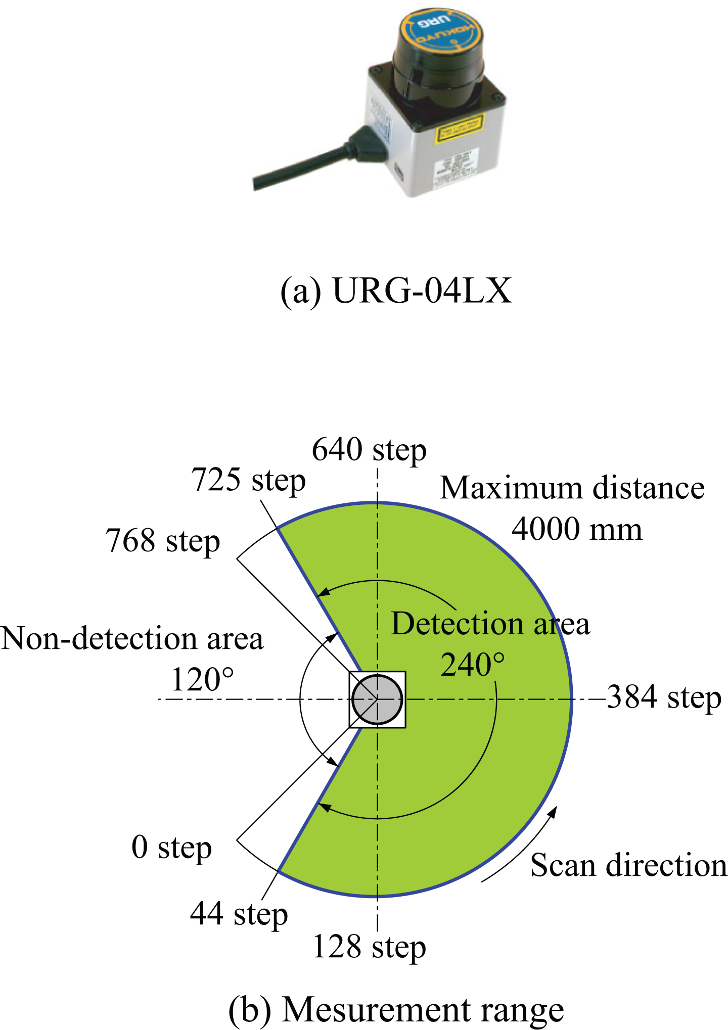
Figure of laser range sensor URG-04LX (Hokuyo Automatic Co., Ltd) and measurement range.

Table 1.

Laser range sensor for simulation.

Laser range sensor	Simulated model of URG–04LX
Distance range	60–4000 mm
Accuracy	20–1000 mm: ±25 mm
	1000–4000 mm: ±2.5%
Distance resolution	3.84 mm ((4000-60) mm/1024)
Scan angle	240°
Angular resolution	1.875° (240°/128)

The details of the SLAM algorithm can be found in the study by Ravankar et al., ³⁰ but what is relevant to the proposed idea is that the robot can estimate the errors in x, y, and orientation φ at each step. Figure 12 shows the result of localization and mapping at a particular step in which the constructed map is shown by small “+” mark in pink color. Sensor location is shown by a larger “+” sign in pink color, and similarly sensor orientation is shown by an arrow.

Figure 12.

Result of pheromone deposition while localizing in map.

Figures 13, 14, and 15 show the estimation errors in φ, x, and y, respectively, at each step of the robot, along with the respective true and the estimated values. As mentioned earlier, pheromone deposition is scalar in nature, that is, the robot can deposit pheromones at the same place irrespective of its orientation. Hence, the orientation in uncertainty is not considered. The errors estimated in x and y are a direct reflection of the spatial uncertainty of the robot in the map. Figure 16 represents the combined error of this spatial uncertainty at each step of robot, where the robot took a total of 124 steps in the experiment. It can be seen that at the start of the operation, the uncertainty of the robot is zero, and it starts to vary as the robot moves in the environment.

Figure 13.

Estimation error of sensor angle φ.

Figure 14.

Estimation error in X-axis.

Figure 15.

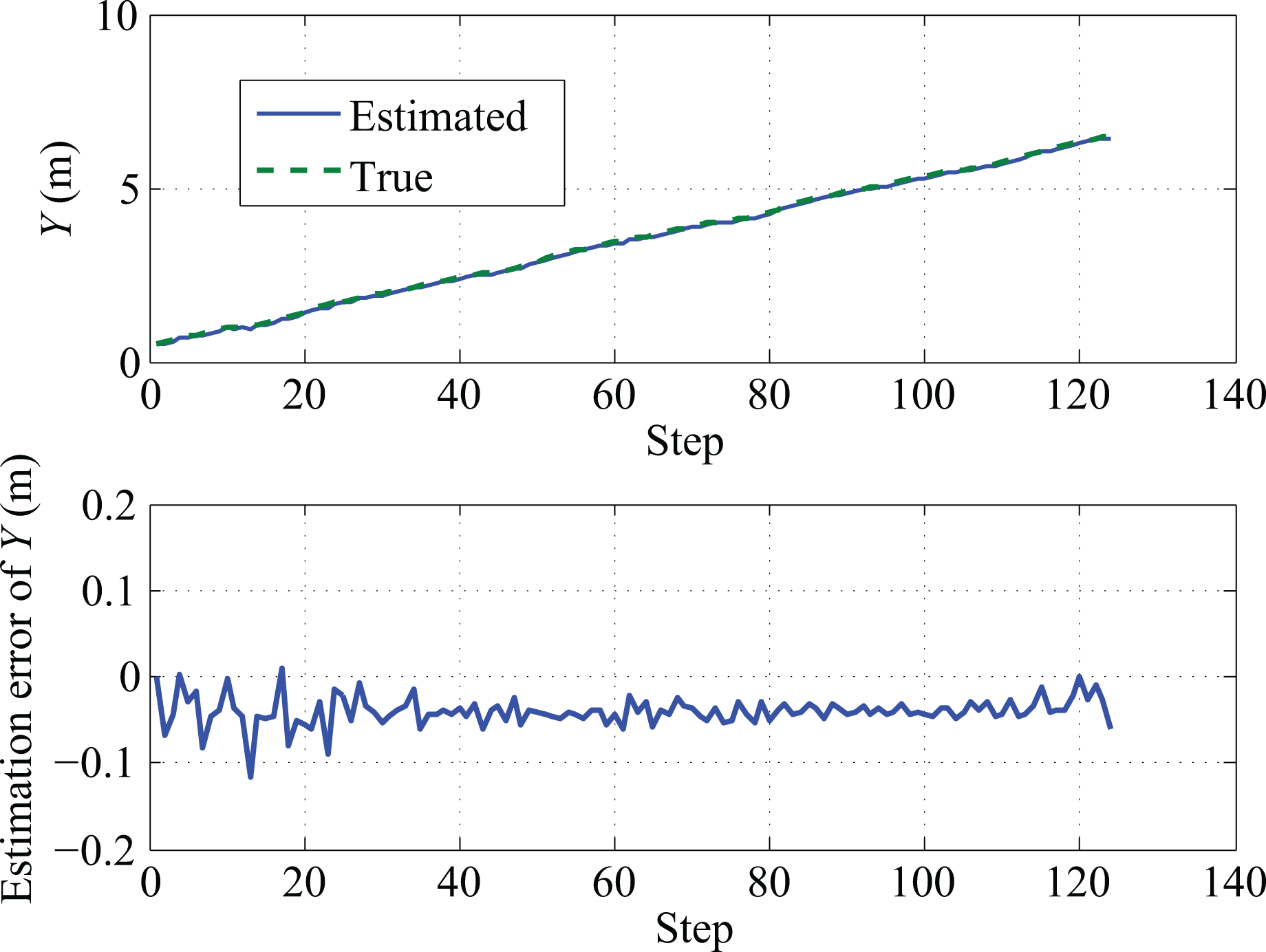
Estimation error in Y-axis.

Figure 16.

Combined error representing spatial uncertainty.

Figure 17 shows the total number of pheromones deposited by the robot at each step. The parameter γ in equation (12) was set to 0.2. A zero uncertainty at the start of the operation would result in an infinite pheromone deposition by equation (12) but an upper limit of 100 was set for the maximum number of pheromones which could be deposited in the map. For a comparative analysis, Figure 18 shows the positional uncertainty of the robot and the pheromones deposited at each step, in the same graph. The amount of pheromones are shown in a log–log scale, whereas the uncertainty is scaled up three times. It can be seen in Figure 18 that at the start of the operation with no uncertainty, the robot deposits a maximum (100) number of pheromones. It can also be seen in Figure 18 that, the peaks in uncertainty of the robot (shown in green color) correspond to the drops in the amount of pheromones deposited (shown in red color). This means that robot had deposited less pheromones at uncertain locations. On the other hand, drops in the uncertainty maps well to the peaks in the pheromones deposited, at any step. This validates that the robot deposited more pheromones at locations with good localization.

Figure 17.

Value of pheromones deposited.

Figure 18.

Comparison of pheromones and uncertainty.

Results in real environment

For the real environment, we used Pioneer-P3DX ³² and Kobuki Turtlebot ³³ robot shown in Figure 19. Pioneer P3DX was the leader robot, and Turtlebot was programmed to follow the trails of Pioneer P3DX. Living creatures like ants deposit chemical pheromones in the environment. Solutions have been proposed to mimic biology by actually depositing and detecting chemicals by the robots as in the studies by Purnamadjaja and Andrew Russell and Genovese et al. ^34,35 However, such attempts are limited by the cost of physical sensors and are not scalable. Virtual pheromones, which are mostly software counterparts of the chemicals, have also been attempted to be realized using Infrared sensors mounted on the top of mobile robots for pheromone communication. Other researcher have proposed to use radio-frequency identification sensors. ^36,37 In this article, a virtual pheromone deposition similar to the study by Susnea et al. ³⁸ is used. In the present work, virtual pheromones are deposited on a common map located on a central remote server, which is accessible to all the mobile robots. All the robots and the server are on the same wireless network for communication. The map is discretized into small cells of unit area. The estimate robot pose [x y] ^T may have fractional values which are rounded off to the nearest integer values for deposition in cells. Since all the robots deposit the virtual pheromones on the central server, pheromone addition from multiple robots and evaporation easily becomes feasible. This flexibility, however, comes at a cost of frequent communication.

Figure 19.

Robots used in the experiments. (a) Pioneer P3DX, (b) Kobuki Turtlebot, and (c) motion model of two wheel differential drive robots.

It is assumed that the leader and trailing mobile robots start from the same location, which allows them to have the same “anchor” in the global map. This allows the robots to create and maintain a correspondence between the spatial coordinates and features of the map. The situation when multiple robots initialize operation from different points of the map is a different area (multi-robot mapping and localization) of research and not considered in this article. For those scenarios, a relative formulation of the relationship between multiple poses of multiple robots needs to be maintained and solutions have been provided in various previous works. ^{39 –43}

Both the robots had SLAM units to build a map and localize themselves in the cluttered corridor environment as shown in Figure 20 with many similar features. The total length of the corridor was about 36 m and 3 m wide. Grid map of the environment was made using PF and modified standard robot operating system (ROS ⁴⁴ ) mapping library. ⁴⁵ Each robot maintained its own map, and the pheromones calculated were deposited in its own map and the server.

Figure 20.

Real environment.

Motion model

Both Pioneer-P3DX and Turtlebot are two wheeled differential drive robots. We first describe the motion model of the robot. The distance between the left and the right wheel is W_r, and the robot state at position P is given as [x, y, θ]. From Figure 19(c), turning angle β is calculated as

$\begin{array}{l}r=\beta \cdot \left(R+W_r\right)\\ l=\beta \cdot R\\ \therefore \beta =\frac{r-l}{W_r}\end{array}$

27

and the radius of turn R as

$R=\frac{l}{\beta },\beta \ne 0$

28

The coordinates of the center of rotation (C, in Figure 19(c)) are calculated as

$\left[\begin{array}{c}Cx\\ Cy\end{array}\right]=\left[\begin{array}{c}x\\ y\end{array}\right]-\left(R+\frac{W_r}{2}\right)\cdot \left[\begin{array}{c}\text{sin}\theta \\ -\text{cos}\theta \end{array}\right]$

29

The new heading θ′ is

$\theta \prime =\left(\theta +\beta \right) \text{mod} 2\text{π}$

30

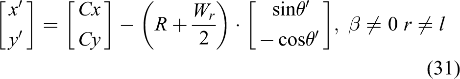
from which the coordinates of the new position P′ are calculated as

$\left[\begin{array}{c}x\prime \\ y\prime \end{array}\right]=\left[\begin{array}{c}Cx\\ Cy\end{array}\right]-\left(R+\frac{W_r}{2}\right)\cdot \left[\begin{array}{c}\text{sin}\theta \prime \\ -\text{cos}\theta \prime \end{array}\right], \beta \ne 0 r\ne l$

31

If r = l, that is, if the robot motion is straight, the state parameters are given as

$\theta \prime =\theta$

32

and

$\left[\begin{array}{c}x\prime \\ y\prime \end{array}\right]=\left[\begin{array}{c}x\\ y\end{array}\right]+l\cdot \left[\begin{array}{c}\text{cos}\theta \\ \text{sin}\theta \end{array}\right], (l=r)$

33

Behavioral difference of follower robot with and without proposed method

A robot may get lost in actual scenarios of cluttered disaster sites due to lack of visibility, noise, and many other factors. However, since the experiment environment (Figure 20) was simple, in order to realize a “leader lost” scenario, the number of particles for the leader robot were purposefully set to a low value. Instead of depositing the pheromones at each and every step, we programmed the robot to deposit the pheromones at intermittent time intervals according to the estimated positional uncertainty in the map. Figure 21 shows the map created by the robot at the start of the operation. The blue ellipses correspond to the spatial uncertainty in robot’s localization. Smaller ellipses reflect smaller uncertainty, and vice versa. Each particle represents a “belief” of the robots pose. The particles are shown in cyan color. The concentration of particles over an area is an indication of how good the localization is. If the particles are densely concentrated in an area, it means that there is less error in estimating the robot’s position in the map. More dispersed particles indicates that the robot is unable to calculate a good estimate of its position.

Figure 21.

Good localization at the start of the operation. Uncertainty in localization is represented by blue ellipses and particles in cyan.

PF can represent multi-modal probability densities. In the present work, it is assumed that the PF models a single hypothesis as the indoor environment used in the experiment has many unique features so that the particles converge quickly after a few scans. In case the environment is devoid of unique features, the PF may generate multiple hypothesis representing multiple possible locations of the robot. In that case, the pheromones will be deposited at multiple estimated positions of the map, some of which will be wrong locations. Once unique features are found and the particles have converged to a single hypothesis, the wrongly deposited pheromones needs to be removed or evaporated quickly. This can be achieved by tracking the number of hypothesis generated by the PF. If it is more than one, the locations of pheromone deposition can be buffered in memory, and later when the particles converge to a single hypothesis the pheromones deposited at wrong locations can be eliminated. However, this case is not considered in the present work and is planned to be addressed in a future extension of the work.

The robot assumes its position to be the mean location of all the particles. The calculation of covariance matrix in case of PF can be found in the literatures. ^{19,20,24 –26} It can be seen that at the start of the operation, there is less uncertainty and all the particles are concentrated over a smaller area as indicated by the size of the ellipses in Figure 21.

Figure 22 shows the uncertainty of the robot at different locations of the map from location L1 to L15. In the 3 m wide corridor, the positional uncertainty of the robot was well within the bounds until location L12. After location L12, the robot was unable to localize well and the uncertainty exceeds the width of the corridor. Figure 23 shows the total number of pheromones deposited at locations L1 to L15. For a long corridor, such as the one used in the experiment, the threshold pheromone value was set to 10 for the trailing robots to catch up with the leader robots. The total number of pheromone deposition at location L11 was 11.35, and at location L12 was 8.15 pheromones, which is below the set threshold.

Figure 22.

Leader (P3DX) robot’s uncertainty at different locations L1 to L15. Uncertainty in localization is represented by blue ellipses and particles in cyan. The uncertainty well within the bounds of the corridor until location L12. After location L12, there is bad localization and minimum number of pheromones are deposited. The robot goes to location A which is highly uncertain location due to large uncertainty of the leader robot.

Figure 23.

Pheromones deposited at different locations shown in Figure 22. Blue areas show pheromones above threshold (10). Total pheromones at location L12 were 8.15.

As indicated in Figure 22, the leader robot explores location A in the map. Since the positional uncertainty of the leader robot is too high, there is a high probability that the robot is exploring wrong area of the site. Figure 24 shows the trajectory of the follower Turtlebot robot. From the point of view of the trailing Turtlebot robot, which sensed a very less amount of pheromones after location L12, Pioneer-P3DX robot was considered “lost.” It can be seen from Figure 23 that the total amount of pheromones deposited is a direct indication of the uncertainty of P3DX for the trailing Turtlebot robot. Turtlebot abandons following the pheromones after location L12. As shown in Figure 24, Turtlebot explores location B and not A.

Figure 24.

Trajectory of the follower robot (Turtlebot). “Leader lost” is detected at location L12 and Turtlebot goes to location B. Blindly following the pheromones using the traditional pheromone deposition schemes would have caused Turtlebot to end up at uncertain location A, which is avoided using the proposed uncertainty modeling.

Notice that, with the traditional pheromone deposition schemes which do not model the uncertainty, Turtlebot would have blindly followed the pheromone trails of the leader robot and ended up at location A of Figure 24, which has high probability of being a wrong area due to the high positional uncertainty of the leader robot. Moreover, all the subsequent follower robots too would have ended in the uncertain location A of the site. However, with the proposed uncertainty modeling, the follower robot can know that the leader was lost at a particular position and can instead explore other areas of the site (like the location B in the experiment).

Results of speed adaptation of trailing robots using the proposed method

While there are many aspects of how the proposed technique improves the efficiency of the system, we consider some practical examples. In search and rescue operations, an indication of higher uncertainty of leader robots is useful for a trailing robot if it fails to find the leader robot at some location and can instead rely on some other important factors rather than the virtual trails themselves. Another important application is in speed adaptation by a trailing robot depending on the intensity of the pheromones encountered at different locations. A trailing robot can increase its speed if it consequently encounters high deposition of pheromones in the map, as it is an indication of being on a good track and the proximity of other robots. On the contrary, if a trailing robot encounters weak and dispersed pheromone trails, then it is an indication of the uncertainty of the leader robots and a large separation between the two. In this case, a trailing robot is supposed to lower its speed for more robust search of the leader robot.

Although experiments regarding pheromone-based speed control of trailing robot are discussed in this section, it does not imply that it should be the only criterion for speed control. Robots must control their speed taking many factors into consideration like the static and dynamic obstacles in the environment, width of the path, visibility (in case of vision sensors), width of the path, steepness and smoothness of the path, intersecting paths with other robots or people, and others.

Figure 25(a) shows the amount of pheromones deposited by the leader robot (first robot). This pheromone deposition is the result of SLAM employed by the robot in Section “Results in simulation environment.” Figure 25(b) shows how the second robot adapts its speed according to the sensed pheromones deposited by the first robot. We set the maximum speed of the robot to 1 m/s. It can be seen that initially (step number 1 to 18), a large pheromones are sensed by the trailing robot and hence its speed is high. However, as the uncertainty increases, the trailing robot reduces its speed, accordingly. Figure 26 shows the speed adaptation by a third trailing robot. Notice that, the second trailing robot also has a SLAM component and will also deposit pheromones on the top of the first robot’s pheromones. Figure 26(a) shows the pheromone deposition by the second robot. Figure 26(b) shows the total pheromones from the first and the second robot with a maximum pheromone threshold of 100. Figure 26(c) shows the adaptation in speed by the third robot according to the total pheromones sensed at each step. Figure 27 shows the example of speed adaptation in real environment. Figure 27(a) shows the total pheromones deposited at the 15 locations on the map of Figure 22. Figure 27(b) shows the adaptation in speed by the trailing robot. For the real environment, we set the speed to specific values according to a range of pheromones described in Table 2.

Figure 25.

Speed variation of the second trailing robot with respect to the pheromones deposited by the first robot (in simulation experiment). (a) Pheromones deposited by the first robot and (b) speed of the second trailing robot.

Figure 26.

Speed variation of the third trailing robot with respect to the total pheromones deposited by the first and second robots (in simulation experiment). (a) Pheromones deposited by the second robot, (b) total pheromones deposited by the first and second robots, and (c) speed of the third trailing robot.

Figure 27.

Speed variation of the trailing Turtlebot robot with respect to the pheromones deposited by Pioneer P3DX robot (in real experiment). (a) Pheromones deposited by Pioneer P3DX robot and (b) speed of trailing Turtlebot robot.

Table 2.

Pheromone range and corresponding robot speed.

Pheromone range	Speed (m/s)
60–100	1
30–60	0.65
15–30	0.45
0–15	0.15

Notice that, a robot can not only adapt its speed but can also turn on/off some sensor modules based on confidence or uncertainty of pheromones sensed at different locations. For example, when it is found that the leader robot is lost, the trailing robot can change parameters of SLAM or sensors (like increase the frames per second of camera), or switch on/off other sensors for more robust search. On the contrary, it can also turn off some features to save computation. A particularly useful case in case of PFs is to increase the number of particles for more robust localization based on the number of pheromones encountered.

Discussion and conclusion

Pheromone trailing is a well-studied phenomenon in robotics and a wide range of applications have successfully been proposed. Traditionally, pheromones have been thought of as static quantities with binary qualities, that is, they just indicate the presence or absence of something. A presence of pheromones indicates that the robot took this path and its absence means that this path has been unexplored. Although a very powerful technique, traditional pheromone trail techniques have largely been limited to simulations. This is mainly because the dynamics and challenges of mobile robots working in fields are immense and hard to model. One such factor is a good localization of the robot in such dynamic environments which is difficult to achieve. Since the location at which pheromones are deposited is very crucial for a multi-robot system employing virtual pheromone trailing, we strongly believe that the positional uncertainty of the robot needs to be modeled in pheromone deposition. This modeling, as proposed in the current work, provides extra information to the trailing robot about the preceding robot. A “confident” deposition concentrated in a small area indicates that the preceding robot was certain about its location at that place. Whereas low and dispersed pheromones indicate that the preceding robot was not sure about its location while depositing pheromones.

We presented a mathematical model of uncertainty modeling in pheromone deposition. We tested the proposed model in both simulation and real environment. The proposed technique will work irrespective of the SLAM technique employed with the robot. Calculating the robot’s positional uncertainty is computationally expensive. However, SLAM is an indispensable component of every mobile robot and it is rare to see mobile robots relying solely on wheel encoder data. The proposed technique can be used in conjunction to any SLAM module to deposit pheromones. The various parameters can experimentally be found using the mathematical model for various environments.

The proposed model can easily be extended to a three dimensional (3-D) case in which an unmanned air vehicle deposits pheromones in 3-D space. Moreover, pheromone deposition in case of multiple hypothesis generation by PF is also considered as potential future work.