Sage Journals: Discover world-class research

Abstract

Predicting depth from a single image is an important problem for understanding the 3-D geometry of a scene. Recently, the nonparametric depth sampling (DepthTransfer) has shown great potential in solving this problem, and its two key components are a Scale Invariant Feature Transform (SIFT) flow–based depth warping between the input image and its retrieved similar images and a pixel-wise depth fusion from all warped depth maps. In addition to the inherent heavy computational load in the SIFT flow computation even under a coarse-to-fine scheme, the fusion reliability is also low due to the low discriminativeness of pixel-wise description nature. This article aims at solving these two problems. First, a novel sparse SIFT flow algorithm is proposed to reduce the complexity from subquadratic to sublinear. Then, a reweighting technique is introduced where the variance of the SIFT flow descriptor is computed at every pixel and used for reweighting the data term in the conditional Markov random fields. Our proposed depth transfer method is tested on the Make3D Range Image Data and NYU Depth Dataset V2. It is shown that, with comparable depth estimation accuracy, our method is 2–3 times faster than the DepthTransfer.

Keywords

Depth extraction single image sparse SIFT flow

Introduction

Depth estimation from a single image is an important issue in 3-D scene understanding. From Figure 1, it is easy for people to understand its 3-D structure; however, it is still a hard task for current computer vision systems to do so, due to lack of reliable cues, such as stereo disparity and motion.

Figure 1.

Depth estimation from a single image: Input images and depth maps estimated by our method. Color indicates depth (red for far and blue for close).

Scene depth is essential for a variety of tasks, ranging from 3-D modeling and visualization to robot navigation. Many challenging computer vision problems have proven ^{1

–5,31,32} to benefit from the incorporation of depth information, such as RGB-D visual odometry,¹ semantic labellings,² pose estimations,³ 3-D shape representation,⁴ and 2.5-D object recognition.⁵

In addition to parametric methods^6

–9 for extracting depths, many nonparametric depth sampling approaches^10,11 have also been proposed to automatically convert monocular images into stereoscopic images with good performances.

Karsch et al.,¹¹ by exploiting the availability of a set of images with known depth, proposed a nonparametric algorithm (DepthTransfer) for depth estimation. Depth in the input image is estimated by first retrieving similar images from this set and then followed by depth warping and fusion. However, the nonparametric depth sampling¹¹ is very slow, which has to spend a lot of time and memories on computing the SIFT flow. Even though the SIFT flow computation is based on a coarse-to-fine scheme, its time complexity is still O(n² logn) (suppose an image has n² pixels). In addition, the weights of the data term in the energy formation in the work of Karsch et al.¹¹ are assigned by comparing pixel-wise SIFT descriptors, which are not discriminative enough for accurate matching during the SIFT flow computation.

In this article, we propose a novel sparse SIFT flow algorithm, which is of sublinear time complexity and much faster than the SIFT flow. In addition, a reweighting technique is introduced where the variance of the SIFT flow descriptor is computed in every pixel and used for reweighting the data term in conditional Markov random fields (CRFs). Our experimental evaluation shows that our depth estimation algorithm not only speeds up the computation but also achieves comparable depth estimation accuracy compared with the original DepthTransfer on the Make3D data set and outperforms state-of-the-art depth estimation approaches on the NYU data set, as demonstrated in section “Experimental evaluations.”

The rest of this article is organized as follows: Section “Related work” introduces the related works. The proposed sparse SIFT flow algorithm and the reweighted confidence are elaborated in section “The proposed approach.” Section “Experimental evaluations” reports the experimental results, and the final section gives the conclusion.”

Related work

Depth extraction from single images has received a lot of attention in recent years. Hoiem et al.⁹ created convincing-looking reconstructions of outdoor images by assuming planar scene composition. Simple geometric assumptions have proven to be effective in estimating the layout of a room.^12,13 Saxena et al.^6,7 predicted depth from a set of image features using linear regression and a CRF and later extended their work into the Make3D⁸ system for 3-D model generation. Their approach first oversegmented the images into many superpixels, and then the 3-D position and orientation of each pixel were inferred via energy minimization under the Markov random field (MRF) framework.

Recently, Fouhey et al.¹⁴ presented an approach to infer 3-D surface normals from a single image using the primitives that were visually discriminative and geometrically informative. They also introduced mid-level constraints for 3-D scene understanding in the form of convex and concave edges in the study by Fouhey et al.¹⁵ Ladicky et al.¹⁶ combined contextual and segment-based cues and built a regressor in a boosting framework by transforming the problem into a regression of coefficients of a local coding. Hane et al.¹⁷ presented an approach to incorporate a surface normal direction classifier into a continuous cut formulation to extract a depth map from unary potentials for different labels. Baig et al.¹⁸ proposed a depth recovery mechanism “im2depth,” which was lightweight enough to run on mobile platforms while leveraging the large-scale nature of modern RGB-D data sets. Konrad et al.¹⁹ proposed a novel depth estimation method that achieved higher performance on indoor scenes.

Convolutional networks have been applied with great success to depth extraction from single images. Eigen et al.²⁰ addressed this task by employing two deep network stacks: one is to make a coarse global prediction based on the entire image and the other is to refine this prediction locally, which can combine global and local information from various cues. Eigen and Fergus²¹ proposed to use a multiscale convolutional network to predict depth from a single image. Wang et al.²² presented a novel convolutional neural network (CNN) architecture for surface normal estimation. Liu et al.^23,24 presented a deep convolutional neural field model based on fully convolutional networks and a novel superpixel pooling method, combining the strength of deep CNN and the continuous CRF into a unified CNNs framework. Li et al.²⁵ estimated the depth from single images by a regression on deep convolutional neural network features combined with a postprocessing refining step using CRF.

Karsch et al.¹¹ used the nonparametric method¹⁰ to infer depth from a single image by exploiting the availability of a set of images with known depths. Depth in the input image was then estimated by first retrieving similar images from this set and optionally warping their depth using the SIFT flow.²⁶ Then, this method combined these warped depth maps into an objective function to smooth the resulting depth. More recently, Liu et al.²⁷ explored continuous variables to represent the depth of image superpixels and discrete ones to encode relationships between neighboring superpixels. The depth estimation was formulated as an inference in a high-order, discrete–continuous graphical model, which is realized using particle belief propagation. Later, the same group²⁸ exploited the structure of the scene at different levels of details to learn depth from a single image.

This article focuses on the classical methods about learning depth from single images, and its mechanisms are different from the deep learning based. DepthTransfer has shown great potential in estimating depth from a single image; however, it requires a lot of time and memories during the SIFT flow computation. In addition, the weights of the data terms are not discriminative enough for accurate matching during the SIFT flow computation. In order to solve these two problems, an accelerating algorithm and a reweighting technique are proposed in this article.

The proposed approach

The proposed approach for pixel-level depth estimation from a single image is outlined in Figure 2. Given a database of the known mapping relationship between RGB images and depth images, a data-driven technique is used to learn the depth of the input RGB image. First, the global generalized search trees (GIST) features are extracted from the input RGB image, and k-NN method is used to search for the most similar k RGB images as candidates in the database. Then, we use the SIFT flow method to encode the dense mapping relationship between the candidate RGB images and the input RGB image and warp the candidate depth images to the input depth image. In order to speed up the computation, a novel sparse SIFT flow method is proposed to replace the classical SIFT flow technique, assuming that the distribution of a depth image is similar to the distribution of the gradient of the converted gray image. The depth estimation is formulated as a maximum a posterior (MAP) problem in the CRFs. In order to further improve the estimation accuracy, we propose a discriminative feature extraction method to reweight the data term of the CRF.

Figure 2.

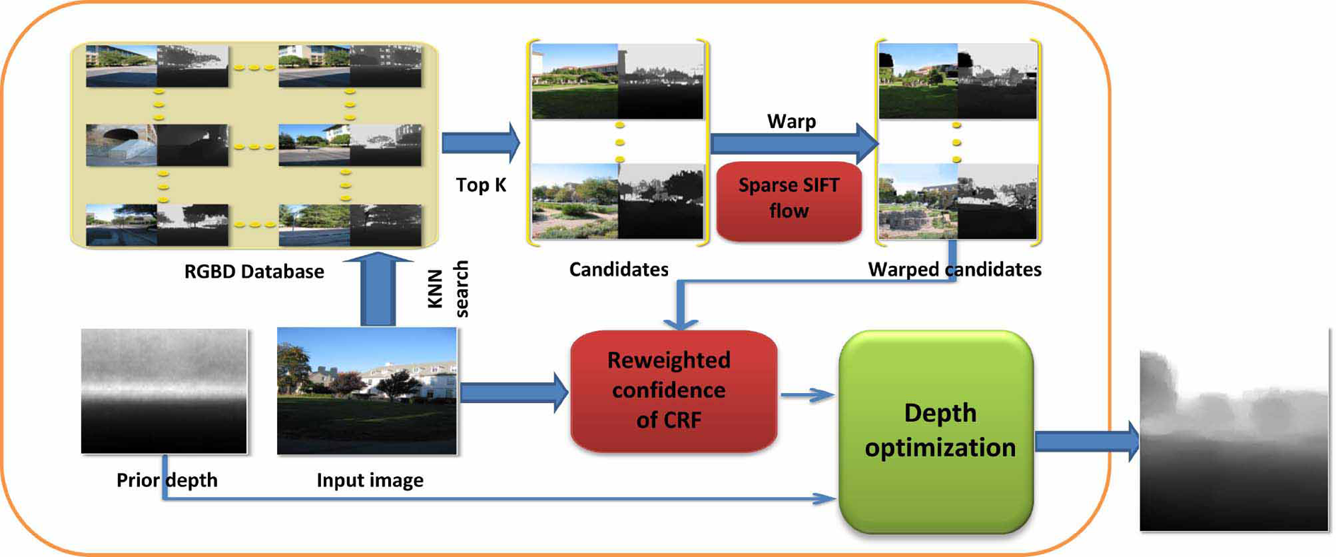
The pipeline of our approach to estimate depth from a single image.

Sparse SIFT flow

SIFT flow²⁶ adopts a coarse-to-fine flow matching scheme to improve the time performance. It first estimates the flow at a coarse level of image grids, then, gradually propagates and refines the flow from coarse to fine. Suppose an image has n² pixels, the complexity of SIFT flow is O(n² logn). In order to reduce the time complexity, instead of using multiple cores or graphic processing unit (GPU) to program, we propose to randomly sample instances, and then, use those instances as a sparse representation. The flow chart of the sparse SIFT flow is shown in Figure 3.

Figure 3.

The sketch map of our sparse SIFT flow.

Given two m × n RGB images, we sample them to form two four-layer pyramids, respectively, as shown in Figure 3. The number of the pyramid layers in the sparse SIFT flow could be greater than or equal to 4. We use publicly available data sets: the Make3D data set and the NYU v2 Kinect data set, whose sizes are 345 × 460 and 480 × 640, respectively. Due to the size of the images in the data sets for estimating depth from single images, the pyramid used in this article is coded to have four levels. In addition, the SIFT flow used in the study by Karsch et al.¹¹ is also coded to have four levels. This computation framework is top-to-bottom. Every pixel of the two images is represented by a 128-dimensional SIFT descriptor. First, we match the top two images with a size of $\frac{m}{8} \times \frac{n}{8}$ by utilizing pixel-wise SIFT descriptor and obtain dense correspondence flow map as “top flow.” When matching the second level with a size of $\frac{m}{4} \times \frac{n}{4}$ , the coarse matching information from the top level is used to reduce the search space. Based on this coarse-to-fine scheme of the SIFT flow, we compute the dense flow map layer by layer, and finally, recover the dense flow of the bottom layer.

To further accelerate the computation, we propose a method to compute the dense flow using a bilinear upsampling from the upper layer to the lower layer, as shown in Figure 3. We implement bilinear interpolation at the second, the third, and the top flows, respectively, and the corresponding results are reported in Table 3. Here, we take the bilinear upsampling of the “second flow” with a size of $\frac{m}{2} \times \frac{n}{2}$ , for example. When computing the “first flow” with a size of m × n, instead of using SIFT descriptors of the image 1 and image 2, we directly employ a bilinear interpolation approach of the “second flow.” In other words, we only use the sampled image with a size of $\frac{m}{2} \times \frac{n}{2}$ to represent the m × n source image. As shown in section “Experimental evaluations,” the sampled $\frac{m}{4} \times \frac{n}{4}$ images and the $\frac{m}{8} \times \frac{n}{8}$ sampled images are also used to implement the bilinear upsampling, contributing to decide which layer is better to implement the bilinear.

Since the SIFT flow²⁶ is dense and smooth, we perform the linear interpolation first in one direction and then in the other direction. In this way, we can preserve the smoothness of the image as shown in Figure 4.

Figure 4.

(a) A Mars satellite image, (b) the same image taken 4 years apart, (c) result of SIFT flow, and (d) result of our sparse SIFT flow.

Below is an example of the bilinear interpolation for the flow map. Given a function f, and four points (0, 0), (0, 1), (1, 0), and (1, 1), the interpolation at (x, y) is

f (x, y) \approx [\begin{matrix} 1 - x & x \end{matrix}] [\begin{matrix} f (0, 0) & f (0, 1) \\ f (1, 0) & f (1, 1) \end{matrix}] [\begin{matrix} 1 - y \\ y \end{matrix}]

Reweighted confidence

The posterior distribution Pr(x|D) for the input image data D over the labelling of the CRF follows a Gibbs distribution and can be written as

P r (x | D) = \frac{1}{Z} \exp (- E (x))

where Z is a normalizing constant and x is a depth map.

Then, an energy function can be formulated as the sum of unary and pairwise potentials

E (x) = \sum_{i \in V} ψ_{i} (x_{i}) + \sum_{i \in V, j \in N_{i}} ψ_{i j} (x_{i}, x_{j})

where i is the i th pixel in the image V and j is the neighbor pixel of i in N_i.

We use the same pairwise potential in CRF and use the same prior term to initialize the depth as in the study by Karsch et al.¹¹ By analyzing the data term in the study by Karsch et al.,¹¹ we find one problem about the weight of the data term. As shown in equation (4), the weight of the data term in equation (3) is a matching score of pixel-wise SIFT descriptor. It is worth noting that the SIFT descriptor in equation (4) is different from the study by Lowe,²⁹ since we do not localize the multiscale space extreme and eliminate the low response. In other words, we use SIFT descriptor to represent every pixel without extracting the SIFT features in the image. When the descriptor is not discriminative, it makes no sense and even yields a wrong result

w_{i}^{(j)} = (1 + e^{(∥ S_{i} - ψ_{j} (S_{i}^{(j)}) ∥ - μ_{s}) / σ_{s}})^{- 1}

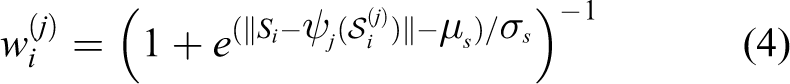
where S_i is the SIFT feature vectors at pixel i in the input image and $S_{i}^{(j)}$ is the SIFT feature vectors at pixel i in the candidate image j.

For the sake of eliminating the wrong matches in SIFT flow, we propose a novel method to identify the best match. As shown in Figure 5(a), it is easy for human to see that AA', BB', and CC' are matching pairs. When we use the SIFT flow, however, AC' and CA' are also considered as potential matching pairs, since the two points are in identical smooth areas, whose SIFT descriptors are approximately same. This is an issue in low discriminative metric. In order to obtain a more reasonable and more accurate estimation, we should increase the matching weight of B and B' and reduce the matching weights of the other two pairs.

Figure 5.

(a) The sketch map of three matching pairs and (b) the distributions of the SIFT flow descriptor in A, B, and C.

Suppose the feature used in equation (4) is not distinctive, we cannot generate a confidence weight to formulate data term even if the matching score is very high. Can we estimate the discrimination by using per pixel feature descriptor? To answer this question, we propose a novel method to reweight the confidence of the CRF by combining distinctive metric of features.

The feature descriptor of a pixel is extracted as follows: the neighborhood of the pixel is divided into a 4 × 4 cell array, the orientation is quantized into eight bins in each cell, and a 4 × 4 × 8 = 128 dimensional vector is obtained as the SIFT representation for a pixel. Intuitively, if the neighboring area is smooth, there will be a single or no peak in SIFT flow descriptor. When the texture of the neighboring area is rich, there will be more than one peak in SIFT flow descriptor. As shown in Figure 5(b), the distribution of the SIFT flow descriptor in the points A and C has no peak and is flat, while the one in the point B has more than one peak. Inspired by this intuition, we use variance to describe the discrimination of the SIFT flow descriptor and then reweight confidence of the data term in the CRFs.

The confidence weight of the data term is redefined as

w_{i}^{(j)} = β v (x_{i}) (1 + e^{(∥ S_{i} - ψ_{j} (S_{i}^{(j)}) ∥ - μ_{s}) / σ_{s}})^{- 1}

where v(x_i) is the variance of the SIFT flow descriptor in pixel i. We set μ_s = 0.5 and σ_s =0.01.

We reweight the confidence of the data term in the CRFs and name it as reweighted confidence.

Experimental evaluations

The experimental computer configuration is 3.7 GHz Intel CPUs with 32 GB memory. The proposed method is tested in both outdoor and indoor scenes. In particular, the proposed method is evaluated using two publicly available data sets: the Make3D data set⁸ and the NYU v2 Kinect data set.³⁰ In addition, the DepthTransfer¹¹ algorithm and two baseline methods are also implemented on the same data sets. We use Matlab, R2014a programming language to implement the referred algorithms. The following three commonly used error metrics are used for quantitative evaluations

Average relative error (rel): $\frac{1}{N} \sum_{i} \frac{| D - D^{*} |}{D^{*}}$

Average $l o g_{10}$ error: $\frac{1}{N} \sum_{i} | l o g_{10} (D) - l o g_{10} (D^{*}) |$

Root mean squared error: $\sqrt{\frac{1}{N} \sum_{i = 1}^{N} {(D_{i} - D_{i}^{*})}^{2}}$

where D denotes the estimated depth, D∗ denotes the ground truth depth, and N denotes the total number of pixels in all images.

Sparsity

In order to study the relationship between the sparsity and the computation cost and learning accuracy, we made a comparison among three sparsity experiments. According to Figure 3, we implement the bilinear interpolation at the second, third, and top flows, respectively, whose sparsity is increasing. The proposed method with different sparsity is tested on the Make 3D database and the NYU v2 Kinect data set, and corresponding results are shown in Figure 6. It is evident that with the increase of the sparsity of the sparse SIFT flow, the computation cost is decreasing, while the estimation accuracy remains almost the same. For the sake of preserving the accuracy of the depth extracted from single images, the second flow is chosen to implement the bilinear upsampling in the following experiments.

Figure 6.

The Make 3D data set and NYU data set are implemented bilinear interpolation at second flow, third flow, and top flow, respectively. (a) Average relative error, (b) average log₁₀ error, (c) root mean squared error, and (d) time performance.

Evaluations on Make3D data set

The Make3D data set contains 534 images with the corresponding depth maps, and it is partitioned into 400 training images and 134 test images. All the images are resized to 460 × 345 pixels in order to preserve the aspect ratio of the original images. The corresponding results by the proposed method and three state-of-the-art algorithms are reported in Table 1, and a plot of the depth errors is shown in Figure 7(a). It is evident that the proposed method is much faster than the DepthTransfer, and the speed-up ratio is about 2.170. At the same time, we achieve similar performance as the DepthTransfer and better performances than Make3d.⁸ Figure 8 provides some qualitative comparisons of our depth maps with those estimated by the DepthTransfer using the data set. It can be seen that the maps estimated by our method and the DepthTransfer¹¹ are visually similar.

Table 1.

Depth reconstruction errors and running times on the Make3D data set.

Method	Rel	log ₁₀	rms	time (h)
Make3D⁸	0.370	0.187	–	–
Discrete–continuous²⁷	0.335	0.137	9.49	–
DepthTransfer¹¹	0.361	0.148	15.146	4.305
ours	0.364	0.152	16.204	1.984

rms: root mean squared; rel: relative error; italics are error metrics, which are used for quantitative evaluations.

Figure 7.

Depth error for DepthTransfer,¹¹ discrete–continuous,²⁷ and the proposed algorithm on the two data sets. (a) Depth errors on the Make 3D data set and (b) depth errors on the NYU data set.

Figure 8.

Qualitative comparison on the Make 3D data set: (first row) four example images, (second row) the corresponding ground-truth, (third row) the corresponding results of the DepthTransfer,¹¹ and (fourth row) the corresponding results of the proposed method.

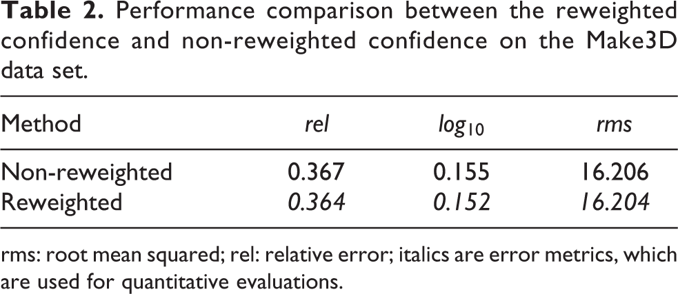
In addition, we evaluated the effectiveness of our reweighted confidence scheme using the Make 3D database. We implement the proposed method with and without the reweighted confidence scheme. The corresponding results are shown in Table 2.

Table 2.

Performance comparison between the reweighted confidence and non-reweighted confidence on the Make3D data set.

Method	rel	log ₁₀	rms
Non-reweighted	0.367	0.155	16.206
Reweighted	0.364	0.152	16.204

rms: root mean squared; rel: relative error; italics are error metrics, which are used for quantitative evaluations.

Evaluations on NYU depth data set

The NYU depth data set consists of 1449 indoor RGB-D images captured using a Kinect. It is randomly partitioned into 1086 training images and 363 test images. Holes from the Kinect are disregarded during training (candidate searching and warping) and are not included in our error analysis.

The proposed method with the sparse SIFT flow and the reweighted confidence is tested on the NYU data set, and the corresponding results are reported in Table 3. In addition, the computation errors and time by Karsch et al.,¹¹ Make3d,⁸ discrete–continuous,²⁷ and Zhuo et al.²⁸ are also reported in Table 3, and a plot of the depth errors is shown in Figure 7(b) at the same time. It is noted that our method is faster than the DepthTransfer, and the speed-up ratio is about 2.10. At the same time, Figure 9 provides some qualitative comparisons of our depth maps with those estimated by the DepthTransfer using the data set. It can be seen that the estimated maps by our method and the DepthTransfer¹¹ are visually very close.

Table 3.

Depth reconstruction errors and running time on the NYU depth data set.

Method	rel	log₁₀	rms	time (h)
Make3d⁸	0.349	–	1.214	–
Discrete–continuous²⁷	0.335	0.127	1.06	–
Zhuo et al.²⁸	0.305	0.122	1.04	–
DepthTransfer¹¹	0.350	0.131	1.223	9.78
Ours	0.357	0.128	1.025	4.65

rms: root mean squared; rel: relative error; italics are error metrics, which are used for quantitative evaluations.

Figure 9.

Qualitative comparison on the NYU data set: (first row) four example images, (second row) the corresponding ground-truth, (third row) the corresponding results of the DepthTransfer,¹¹ and (fourth row) the corresponding results of the proposed method.

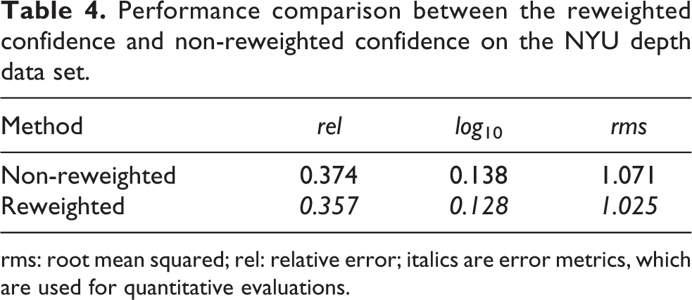
Furthermore, the effectiveness of our reweighted confidence scheme is also evaluated on the NYU database. The proposed method with and without the reweighted confidence scheme is implemented, whose corresponding results are reported in Table 4.

Table 4.

Performance comparison between the reweighted confidence and non-reweighted confidence on the NYU depth data set.

Method	rel	log ₁₀	rms
Non-reweighted	0.374	0.138	1.071
Reweighted	0.357	0.128	1.025

rms: root mean squared; rel: relative error; italics are error metrics, which are used for quantitative evaluations.

Discussion of the reweighted confidence

After implementing the reweighted confidence on the Make 3D data set, the quantitative gains are marginal, as shown in Table 2. However, we show a significant improvement on the NYU v2 Kinect data set with the reweighted confidence scheme, as reported in Table 4. In order to make a clear deep analysis, the variance of every pixel in data sets is computed using the SIFT flow algorithm, as shown in Figure 10. Figure 10(a) shows the average variance of the every test image and Figure 10(b) shows the variance histogram of the every pixel in the test data set. Inspired by Figure 5, the pixel with large variance is weighted with significant confidence, and the small variance pixel is given the small weight, as shown in equation (5). Therefore, the depths estimated from large variance data set could have a big improvement with the reweighting scheme. As shown in Figure 10, the statistical variance of the NYU v2 Kinect data set is higher than the one of the Make 3D, and the average variance of the two data sets is small, which are coincidence with the reweighted confidence scheme. By analysis of the statistical variance of the data sets, the reweighting scheme is helpful in improving the depth accuracy when the variance of images is large.

Figure 10.

(a) The average variance of the every test image and (b) the variance histogram of the every pixel in test data set.

Conclusion

In this article, we have studied the optimization problem of the DepthTransfer by exploiting the availability of a pool of images with known depth. The complexity was reduced from subquadratic to sublinear by the proposed sparse SIFT flow, while preserving the accuracy of the DepthTransfer by reweighting the confidence of the data term. Extensive experimental evaluations demonstrated the effectiveness of the proposed approach. In the future, we will further study the edge depth inference to obtain a more distinctive sketch of scene.

Footnotes

Declaration of conflicting interests

The author(s) declared no potential conflicts of interest with respect to the research, authorship, and/or publication of this article.

Funding

The author(s) disclosed receipt of the following financial support for the research, authorship, and/or publication of this article: This work was supported by the Strategic Priority Research Program of the Chinese Academy of Sciences (XDB02070002) and National Natural Science Foundation of China under grant nos 61421004, 61333015, 61573351, and 61283282.

References

Fang

Zhang

. Experimental evaluation of RGB-D visual odometry methods. Int J Adv Robot Syst 2015; 12: 26.

Ladicky

Shi

Pollefeys

. Pulling things out of perspective. In: Martinez

Basri

Vidal

Fermuller

(eds) Proceedings of the IEEE conference on computer vision and pattern recognition, New York, USA, 24–27 June 2014, pp. 89–96. IEEE.

Shotton

Girshick

Fitzgibbon

. Efficient human pose estimation from single depth images. IEEE Trans Pattern Anal Mach Intell 2013; 35(12): 2821–2840.

Song

Khosla

. 3D shapenets: a deep representation for volumetric shapes. In: Grauman

Learned-Miller

Torralba

Zisserman

(eds) Proceedings of the IEEE conference on computer vision and pattern recognition, New York, USA, 7–12 June 2015, pp. 1912–1920. IEEE.

Song

Xiao

. Sliding shapes for 3D object detection in depth images. In: Fleet

Pajdla

Schiele

Tuytelaars

(eds) Proceedings of the European conference on computer vision, Berlin, Germany, 6–12 September 2014, pp. 634–651. Springer.

Saxena

Chung

SH,

. Learning depth from single monocular images. Adv Neural Inf Process Syst 2005; 18: 1161–1168.

Saxena

Chung

. 3-D depth reconstruction from a single still image. Int J Comput Vis 2008; 76(1): 53–69.

Saxena

Sun

A Y

. Make3D: learning 3D scene structure from a single still image. IEEE Trans Pattern Anal Mach Intell 2009; 31(5): 824–840.

Hoiem

Efros

AA,

Hebert

. Automatic photo pop-up. ACM Trans Graph (TOG) 2005; 24(3): 577–584.

10.

Liu

Yuen

Torralba

. Nonparametric scene parsing via label transfer. IEEE Trans Pattern Anal Mach Intell 2011; 33(12): 2368–2382.

11.

Karsch

Liu

Kang

. Depth transfer: depth extraction from video using non-parametric sampling. IEEE Trans Pattern Anal Mach Intell 2014; 36(11): 2144–2158.

12.

Schwing

Urtasun

. Efficient exact inference for 3D indoor scene understanding. In: Fitzgibbon

Lazebnik

Perona

Sato

Schmid

(eds) Proceedings of the European conference on computer vision, Berlin, Germany, 7–13 October 2012, pp. 299–313. Springer.

13.

Hedau

Hoiem

Forsyth

. Thinking inside the box: using appearance models and context based on room geometry. In: Daniilidis

Maragos

Paragios

(eds) Proceedings of the European conference on computer vision, Berlin, Germany, 5–11 September 2010, pp. 224–237. Springer.

14.

Fouhey

Gupta

Hebert

. Data-driven 3D primitives for single image understanding. In: Kutulakos

Torr

Seitz

(eds) Proceedings of the IEEE International Conference on Computer Vision, New York, USA, 1–8 December 2013, pp. 3392–3399. IEEE.

15.

Fouhey

Gupta

Hebert

. Unfolding an indoor origami world. In: Fleet

Pajdla

Schiele

Tuytelaars

(eds) Proceedings of the European conference on computer vision, Berlin, Germany, 6–12 September 2014, pp. 687–702. Springer.

16.

Ladicky

Zeisl

Pollefeys

. Discriminatively trained dense surface normal estimation. In: Proceedings of the European Conference on Computer Vision, 2014, pp. 468–484. Springer.

17.

Hane

Ladicky

Pollefeys

. Direction matters: depth estimation with a surface normal classifier. In: Grauman

Learned-Miller

Torralba

Zisserman

(eds) Proceedings of the IEEE Conference on Computer Vision and Pattern Recognition, 2015, pp. 381–389. IEEE.

18.

Baig

Jagadeesh

Piramuthu

. Im2depth: scalable exemplar based depth transfer. In: Scheirer

Yang

Stewart

(eds) Proceedings of the IEEE winter conference on applications of computer vision, New York, USA, 24–26 March 2014, pp. 145–152. IEEE.

19.

Konrad

Wang

Ishwar

. Learning-based, automatic 2D-to-3D image and video conversion. IEEE Trans Image Process 2013; 22(9): 3485–3496.

20.

Eigen

Puhrsch

Fergus

. Depth map prediction from a single image using a multi-scale deep network. Adv Neural Inf Process Syst 2014: 2366–2374.

21.

Eigen

Fergus

. Predicting depth, surface normals and semantic labels with a common multi-scale convolutional architecture. In: lkeuchi

Schnorr

Sivic

Vidal

(eds) Proceedings of the IEEE international conference on computer vision, New York, USA, 11–18 December 2015, pp. 2650–2658. IEEE.

22.

Wang

Fouhey

Gupta

. Designing deep networks for surface normal estimation. In: Grauman

Learned-Miller

Torralba

Zisserman

(eds) Proceedings of the IEEE conference on computer vision and pattern recognition, New York, USA, 7–12 June 2015, pp. 539–547. IEEE.

23.

Liu

Shen

Lin

. Deep convolutional neural fields for depth estimation from a single image. In: Grauman

Learned-Miller

Torralba

Zisserman

(eds) Proceedings of the IEEE conference on computer vision and pattern recognition, New York, USA, 7–12 June 2015, pp. 5162–5170. IEEE.

24.

Liu

Shen

Lin

. Learning depth from single monocular images using deep convolutional neural fields. IEEE Trans Pattern Anal Mach Intell 2016; 38: 2024–2039.

25.

Shen

Dai

. Depth and surface normal estimation from monocular images using regression on deep features and hierarchical CRFs. In: Grauman

Learned-Miller

Torralba

Zisserman

(eds) Proceedings of the IEEE conference on computer vision and pattern recognition, New York, USA, 7–12 June 2015, pp. 1119–1127. IEEE.

26.

Liu

Yuen

Torralba

. Sift flow: dense correspondence across scenes and its applications. IEEE Trans Pattern Anal Mach Intell 2011; 33(5): 978–994.

27.

Liu

Salzmann

. Discrete-continuous depth estimation from a single image. In: Martinez

Basri

Vidal

Fermuller

(eds) Proceedings of the IEEE conference on computer vision and pattern recognition, New York, USA, 24–27 June 2014, pp. 716–723. IEEE.

28.

Zhuo

Salzmann

. Indoor scene structure analysis for single image depth estimation. In: Grauman

Learned-Miller

Torralba

Zisserman

(eds) Proceedings of the IEEE conference on computer vision and pattern recognition, New York, USA, 7–12 June 2015, pp. 614–622. IEEE.

29.

Lowe

. Distinctive image features from scale-invariant keypoints. Int J Comput Vis 2004; 60(2): 91–110.

30.

Silberman

Hoiem

Kohli

. Indoor segmentation and support inference from RGBD images. In: Fitzgibbon

Lazebnik

Perona

Sato

Schmid

(eds) Proceedings of the European conference on computer vision, Berlin, Germany, 7–13 October 2012, pp. 746–760. Springer.

31.

Liu

Chen

Zhou

. Single image haze removal via depth-based contrast stretching transform. SCIENCE CHINA Information Sciences 2015; 58(1): 1–17.

32.

Hao

Chen

. Image completion with perspective constraint based on a single image. SCIENCE CHINA Information Sciences 2015; 58(9): 1–12.

Fast depth extraction from a single image

Abstract

Keywords

Introduction

Related work

The proposed approach

Sparse SIFT flow

Reweighted confidence

Experimental evaluations

Sparsity

Evaluations on Make3D data set

Evaluations on NYU depth data set

Discussion of the reweighted confidence

Conclusion

Footnotes

Declaration of conflicting interests

Funding

References