Sage Journals: Discover world-class research

Abstract

Learning from demonstration plays an important role in enabling robot to acquire new behaviors from human teachers. Within learning from demonstration, robots learn new tasks by recognizing a set of preprogrammed behaviors or skills as building blocks for new, potentially more complex tasks. One important aspect in this approach is the recognition of the set of behaviors that comprises the entire task. The ability to recognize a complex task as a sequence of simple behaviors enables the robot to generalize better on more complex tasks. In this article, we propose that primitive behaviors can be taught to a robot via learning from demonstration. In our experiment, we teach the robot new behaviors by demonstrating the behaviors to the robot several times. Following that, a long short-term memory recurrent neural network is trained to recognize the behaviors. In this study, we managed to teach at least six behaviors on a NAO humanoid robot and trained a long short-term memory recurrent neural network to recognize the behaviors using the supervised learning scheme. Our result shows that long short-term memory can recognize all the taught behaviors effectively, and it is able to generalize to recognize similar types of behaviors that have not been demonstrated on the robot before. We also show that the long short-term memory is advantageous compared to other neural network frameworks in recognizing the behaviors in the presence of noise in the behaviors.

Keywords

Behavior recognition LSTM deep learning neural network

Introduction

Learning from demonstration

Robots learning new tasks from human demonstration is inspired by how humans learn new tasks by having experts guiding them. Consider a toddler learning to write an alphabet with the help of an adult guiding the toddler by holding his or her hand. With enough repetition or practice, the toddler is able to master the tasks of writing the alphabet. At this point, the toddler is able to perform the alphabet writing task independent of any guidance from the adult. Eventually, the toddler may even write different variations of the same alphabet learned and still know it is the same alphabet. Once at this stage, it is said that toddler’s learning is successful in the sense that the toddler does not memorize exactly the alphabet that was taught but is able to generalize the concept and reproduce the same type of alphabet that the teacher has not taught.

In the field of learning from demonstration (LfD), the same concept is applied to teach robots new tasks or behaviors. Many researches in LfD encountered problems in generating behaviors from skills or data sampled during demonstrations.¹ One of the most crucial problem is generalization of the behaviors taught during the demonstration. A good generalization of a behavior can be seen as the ability of the robot to repeat the demonstrated behavior in circumstances that are not completely similar during demonstration time. A number of researches agreed that one common way to overcome this is to transform the demonstration into a set of preprogrammed higher-level actions called subtasks, motion primitives, motor primitives or motor skills.^2,3 This transformation supports not only generalization purposes but also as an intuitive way for humans to understand demonstrated data. A labeled sequence of skills, for example, following the wall to my right, passing through a door, going straight over the floor avoiding any obstacle, is significantly easier to interpret than the raw sensor and motor data.¹ Recognition of these individual behaviors in a complex task gives humans the advantage of probing into the interpretation of the robot in response to some raw sensor data. In order to achieve this transformation of raw sensor data into labels, it is a prerequisite to identify or recognize the behavior themselves.

One practical example as a motivation for the recognition of behaviors or skills is highlighted by Hafner et al.⁴ In this work, the authors attempted to generate stable walking gaits for humanoid robots by learning them from the walking gaits of human subjects. Nine 3-axis accelerometers were attached to the specific positions of the human body and the humanoid robot to capture the raw data in a walking task of both the human and the robot. The objective of the work is to allow the humanoid robot to imitate the walking gaits by learning from the demonstrations shown to them. This is analogous to LfD in which a robot learns complex tasks from multiple demonstrations. In agreement to statements by other researchers, Hafner et al. reported that it is important for a humanoid robot to first recognize its own behaviors in order to imitate the behaviors of its human teachers. Recognition of its own behavior allows the humanoid robot to analyze the behaviors and draw a connection between executed and recognized behaviors.⁴ The importance of behavior recognition on a robot remains a central motivation in our study throughout. This study will focus on methods that can be used as a behavior recognition mechanism on a robot.

Neural networks in behavior recognition task

In our study, primitive behaviors are demonstrated on the robot via LfD. In our case, the primitive behaviors consist of encoder values from the joints of the NAO humanoid robot.⁵ The encoder readings specify the absolute position of all joints onboard the NAO robot at any time. Whenever a movement is performed on the robot within a time frame, these encoder values form a sequence of instantaneous values of encoder readings. Figure 1 shows a sample reading from the encoders when a behavior is demonstrated on the robot within a 100-time-step time frame.

Figure 1.

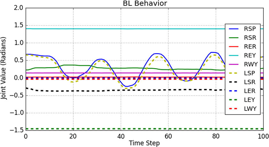
Sample readings from 10 different encoder sensors. Legend shows different joint positions on-board the NAO robot.

Due to the complex nature of the primitive behavior sequences, simple conditioning or thresholding of the encoder values does not work well. Other techniques such as template matching is tedious to implement as we need to hand engineer the features that pertain to specific behavior sequences. Additionally, hand-engineered features only fit particular behaviors and does not generalize well to new behaviors. Template matching also has been shown to be outperformed by other methods such as support vector machines (SVMs) and neural networks on various tasks.

This motivates the use of neural networks algorithm as a method of behavior recognition. Neural network algorithms have been known to outperform many other methods when there is an abundance of data available. It is also shown that neural network is able to learn features from the data⁶ with minimal human intervention. On top of that, recent breakthroughs in deep learning approach involve the use of deep neural networks that have shown to outperform many other algorithms⁷ on various tasks. At the point of this writing, deep learning algorithm has obtained state-of-the-art results in vision-related tasks,⁸ speech recognition,⁹ and many more.

Within the many deep learning techniques, the recurrent neural network (RNN) is of particular interest to us. This is because RNNs are known to handle sequential data very well. Examples of sequential data include audio speeches, textual conversations, stock market prices, and in our case robot encoder readings that pertain to behaviors. Since this study deals with sequential data from encoder readings, the use of RNN is appropriate. However, we also compare the performances of the RNNs to that of the regular feedforward types such as the multilayer perceptron (MLP) and the time-delay neural network (TDNN).

Long short-term memory

The long short-term memory (LSTM) is one of the many variations of the RNN. The LSTM is pioneered by Hochreiter and Schmidhuber.¹⁰ The concept of LSTM is similar to that of an RNN except that instead of having sigmoidal units in the hidden layer, a more complex unit known as “memory units” are introduced. The reason behind the introduction of these memory units is because RNN suffers from a condition known as the vanishing gradient point. This condition causes the information from past events to be lost and overwritten by more recent information. In the study by Graves,¹¹ it is reported that RNNs can only retain information up to only 10 time steps in the past. This is a serious drawback to the RNN because most sequential data store information in sequence length that far exceeds 10 time steps. Therefore, in theory, RNNs cannot be used to compute sequences that are longer than 10 time steps because the information far past in the sequence is lost during the computation.

The LSTM claims to remedy the problem of vanishing gradient by having the memory unit retain the information for an arbitrary amount of time.¹² A typical LSTM memory unit contains gates that determine when an information is significant enough to remember, when it should retain the value in the memory, when it should forget the retained information, and when should it output the value to the next computational unit.

Figure 2 shows a typical LSTM memory cell.

Figure 2.

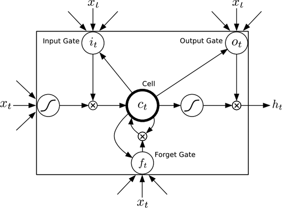
A typical LSTM memory unit consists of input gate, forget gate, output gate, and the cell state.¹² LSTM: long short-term memory.

For most RNN, the hidden layer function, H, is an elementwise application of a sigmoid function (1/1 + e^−x) over the inputs

h_{t} = H (W_{x h} x_{t} + W_{h h} h_{t - 1} + b_{h})

y_{t} = W_{h y} h_{t} + b_{y}

where the W terms denote weight matrices (e.g. W_xh is the input-hidden weight matrix), the b terms denote bias vectors (e.g. b_h is the hidden bias vector), and H is the hidden layer function.

For the LSTM, however, H is implemented in a series of equation involving all the gates as in Figure 2. The implementation of H is given by

i_{t} = σ (W_{x i} x_{t} + W_{h i} h_{t - 1} + W_{c i} c_{t - 1} + b_{i})

f_{t} = σ (W_{x f} x_{t} + W_{h f} h_{t - 1} + W_{c f} c_{t - 1} + b_{f})

c_{t} = f_{t} c_{t - 1} + i_{t} tanh (W_{x c} x_{t} + W_{h c} h_{t - 1} + b_{c})

h_{t} = o_{t} tanh (c_{t})

where σ is the logistic sigmoid function; i, f, o, and c are the input gate, forget gate, output gate, and cell activation vectors, respectively; and W’s are rectangular weight matrices. The output vector sequence y_t is calculated as in equation (2). As shown, the only change is in the hidden layer activation, H.

LSTMs have been widely used to solve many problems related to sequential data and obtained state-of-the-art performances. These includes handwriting recognition,¹³ language modeling,¹⁴ language translation,¹⁵ acoustic modeling of speech,¹⁶ speech synthesis,¹⁷ protein secondary structure prediction,¹⁸ analysis of audio,¹⁹ and video data²⁰ among others.

Related works

Under the literature of robot behavior recognition, several approaches were documented. This includes variance thresholding of certain sensor modalities,^21,22 thresholding the mean velocity of joints,^23,24 and matching of pre- and postconditions with current sensory states.²⁵ SVM is also being proposed for body posture recognition.²⁶ Nearest neighbor classifier is proposed in the study of Bentivegna²⁷ to identify skills in a marble maze task. Learning Vector Quantization²⁸ in combination with nearest neighbor classifier is proposed in the study by Pook and Ballard² to classify sliding windows of data. In the study by Park et al.,²⁹ a hidden Markov model is proposed to recognize the gestures of humans based on the hands and head position using a camera. Even though many of the proposed techniques work well in recognizing many specific behaviors, none provide a general solution to the problem. Behavior recognition also appears to be ill-posed when seen as a classification problem.³⁰

In addition to the above, Billing and Hellström suggested three additional techniques for the recognition of behaviors in mobile robots.¹ In his first technique known as β-comparison, the algorithm compares the output of a controller in response to the input with observed actions in the demonstration. In his experiments, the authors recognize behavior of the mobile robots by comparing the learned behaviors to the behaviors produced by the controller. In the β-comparison algorithm, the learned behaviors are considered to be similar to the one produced by the controller if both produce similar actions given a similar input. The authors, however, reported poor performance of this method because the β-comparison algorithm only compares action vectors.¹

In the second technique, Billing and Hellström proposed the use of autoassociative neural networks (AANNs) for comparison of behaviors. In this technique, a feedforward neural network is implemented where the input and the output of the network are the same to the input. However, the hidden layer of the network is restricted to be small. The network is then allowed to learn the input–output mappings through a small hidden layer. The network is trained by a least squared criterion. Next, the network is presented with new independent behavior data. The similarity of the new data to the training data is evaluated by the reconstruction error value. If the reconstruction error is low, the new data is considered to be similar to the training data. The author reports a reasonable if not the best result in the study by Billing and Hellström.¹

In the third technique, the author proposed the S-comparison algorithm that is based on S-learning, inspired by the human neuromotor system.^31,32 S-learning differs from the previous technique in which β-comparison and the AANN network treat each sample separately as independent events, whereas S-comparison is able to extract temporal patterns and correlation in the behavior data. This allows for the S-learning algorithm to recognize behaviors based on recent observation of data values. Even though S-learning uses the most information from the data, the authors reported no improvement in performance. Several issues are also reported to have affected the performance of the S-comparison in the study by Billing and Hellström.¹

Another different work by Chalodhorn et al.³³ utilized nonlinear principal components analysis (NLPCA) as a mechanism for recognizing behaviors of a humanoid robot involving 25 degrees of freedom (all joints on the robot except two neck joints, two hand joints, and one torso joint). In this work, the authors constructed an NLPCA autoencoder neural network to reduce the number of features in a ball tracking motion of a humanoid robot to only three principal components. The authors approached the problem of behavior recognition using the unsupervised learning method of NLPCA. From the results, the authors manage to successfully recognize five of six types of behaviors without any prior knowledge of the behaviors. The NLPCA algorithm works by clustering similar motions together and thus enables the recognition of the behavior types. However, the authors also noted that the algorithm was not able to distinguish behavior patterns that differ in frequency, for example, fast walking gait and slow walking gait. Figure 3 shows the recognized behaviors in the feature space.

Figure 3.

Recognized motion patterns projected in the first three principal components of the raw data.³³ Legend indicates the type of behaviors modeled in the feature space.

In a more recent paper by Noda et al.,³⁴ the authors utilized deep learning techniques for behavior recognition on a humanoid robot. The approach is somewhat similar to the AANN technique by Billing and Hellström with additional modifications. First, the neural network model consists of 11-layer deep autoencoder neural network compared to the AANN technique with only single hidden layer. The deep autoencoder network by Noda et al. is also modified to handle time-series data by including sliding windows in the input vectors. The novel method combines the TDNN in a 11-layer deep autoencoder configuration allowing the network to process temporal information. Noda et al. used the unsupervised learning method as an approach to classify the behaviors. By utilizing higher level features that can be extracted in the deeper layers of the deep autoencoder, the complexity of classification of the behaviors is reduced dramatically. The authors claimed that the higher level features self-organize in the feature space and form clusters according to the types of behaviors. From this point on, any simple classification algorithm is able to classify the high-level features accurately. In the implementation of TDNN, the algorithm manages to classify as many as six object manipulation behaviors. The results from the experiment show the features of the multimodal data self-organize in the feature space. In this study, the authors showed that the recognition of complex sequence of behavior data can be dramatically reduced using higherlevel features instead of raw data. Figure 4 shows the described high-level feature space documented by Noda et al.

Figure 4.

Multimodal feature space acquired by Noda et al.^34,35 Legend indicates the number of behaviors modeled in the feature space. The feature space shows the behaviors in its three principal components labeled PC1, PC2, and PC3.

The use of the deep neural network in the TDNN by Noda et al. approach has seen great successes in recognizing a number of tasks.³⁴ However, the use of TDNN requires the hyperparameters of the network to be fixed and determined beforehand. One crucial example that is also highlighted in the study is the predetermination of the sliding time window, T. The sliding time window in the implementation of TDNN determines how much contextual information should the network consider for computation. In the study, the authors predetermined the value of the sliding time window, T, to be T = 30 time steps. The main reason of choosing the value is because the authors noted that 30 time steps are enough to characterize one phase of all the behaviors.³⁴ Therefore, T = 30 is an optimized value for all the six behaviors tested in the article. On another note, the authors stated that it is crucial to select an optimized sliding window value, T. If the sliding time window, T, is too small, the network may not learn anything. On the other hand, if the time window is too large, the network may consider more contextual information, and this increases computation time and cost.³⁴ In many cases, the value of the sliding time window, T, is extremely task dependent. There is no value of T that will fit for general use. Therefore, the predetemination of the sliding window value in TDNN would require prior knowledge of the tasks. This would be impractical in some situations where we have no prior knowledge of the task at hand.

In order to eliminate the need to predetermine the sliding time window, T, we embark on a different approach of using RNNs for the task of behavior recognition. The use of recurrent variant of neural networks eliminates the need to determining the value of T. We saw that the value of T dictates how much information does the network retain from past events in order to make a decision on the current event. However, in recurrent networks, how much memory the network retains from past events are learned directly from the data itself. There is no need for human observers to study the data sequences and set the value of T to fit and function well on the sequences. This way, we see the potential of RNNs to be used as a behavior recognition mechanism.

Recurrent networks, especially the LSTM variant, are known to solve many sequence recognition problems in various domains. However, to date, there are no prominent frameworks on using RNN especially LSTM for behavior recognition on robots. Therefore, we are determined to push through our framework of using recurrent networks as a competitive approach to conventional feedforward architecture in the scope of behavior recognition. Therefore, in this study, we particularly explored the performance comparison among recurrent and feedforward neural architecture. We elaborate on the various architectures of neural networks and how it fits into the application of behavior learning in the upcoming sections.

Methodology

Based on the motivation, we carry out our work by utilizing neural networks toward the goal of recognizing primitive behaviors on the NAO humanoid robot. It is shown previously in Figure 1 that each behavior demonstration can be observed as a time series or a sequence. Based on this fact, we approach the problem of behavior recognition as a form of sequence labeling task using the supervised learning scheme. In using supervised learning, each behavior sequence in the data set is given a label. These sequence–label pair is then used as training examples for the neural networks.

Data collection

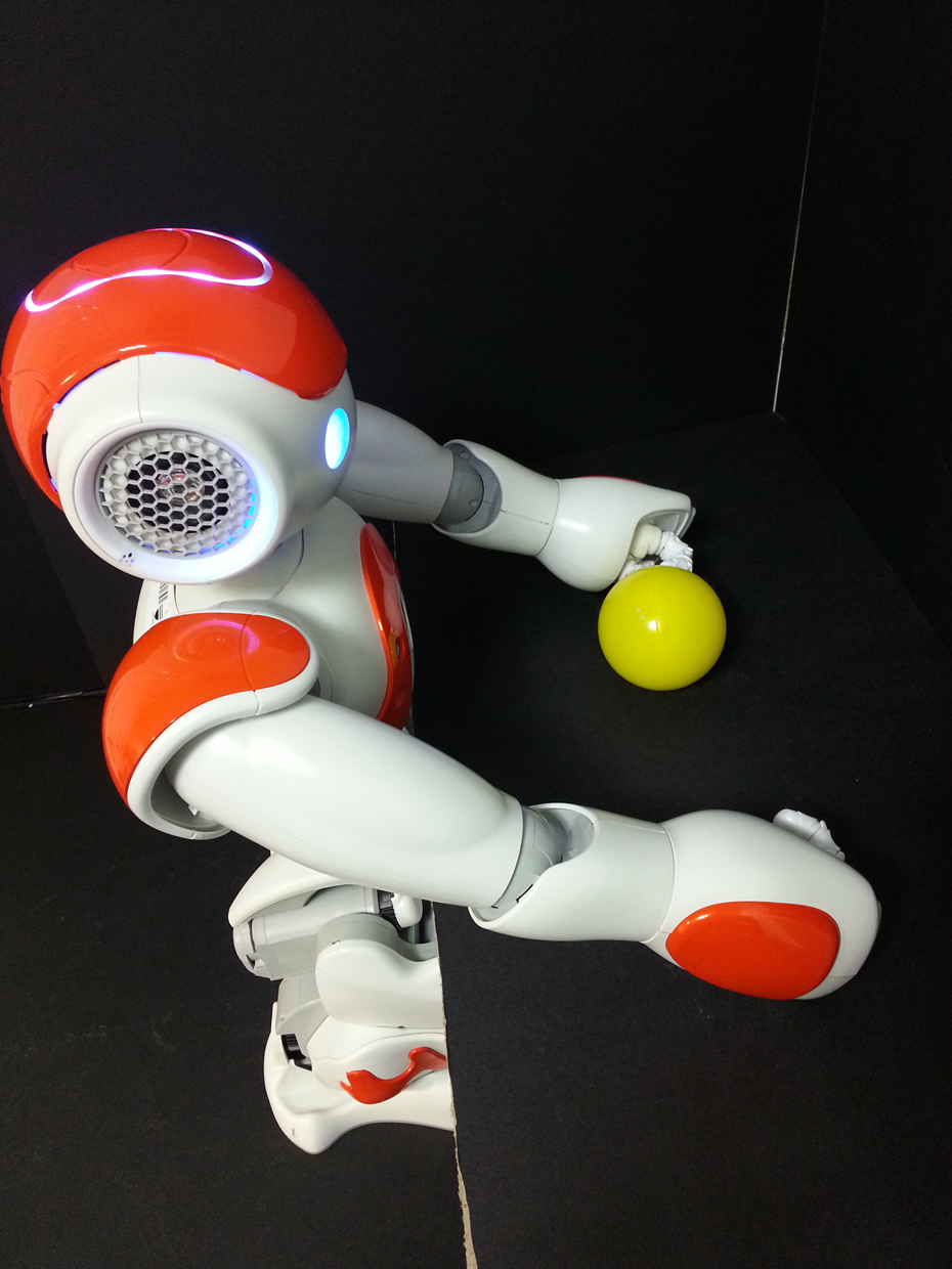
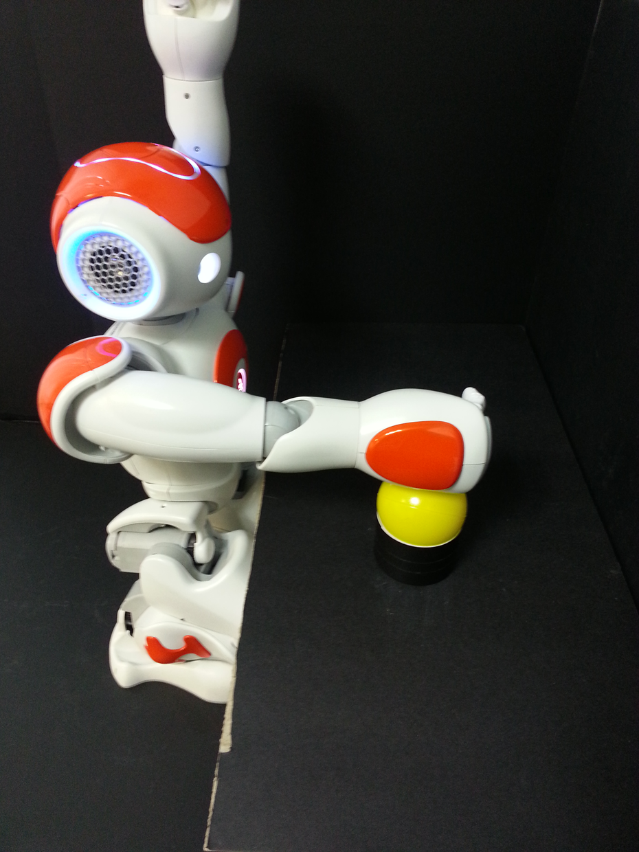
There are no readily available, prominent data set for the task of behavior recognition using the NAO robot to date. Therefore, we decided to sample a data set of primitive behaviors. The behaviors are adapted from the study by Noda et al.³⁴ Sampling is done by demonstrating the behavior on the NAO robot while recording the encoder values from each joint. For simplicity, we only sample from encoders that are located on both arms of the NAO robot. Encoder values from other joints of the NAO robot are not considered. In total, we sampled encoder readings from 10 distinct joints from both the arms of the NAO robot. Table 1 tabulates the name of the joints, its abbreviation, and its respective mathematical notation. Figures 5 to 10 illustrate the six types of primitive behaviors that we demonstrate on the NAO robot. The description of the behaviors is as follows. The ball lift is described as NAO robot holding a yellow ball on a table and raising the ball to shoulder height. The ball roll behavior is described as iteratively rolling a yellow ball on top of a table to the right and left using alternative arm movement. The bell ring left/right behavior is described as hitting a yellow bell on the left/right of the robot using its left/right arm, respectively. The ball roll on a plate is described as rolling a yellow ball on a plate by swinging the left and right arms. The behavior ropeway is described as swinging a white toy from string attached to both hands by moving both arms up and down.

Table 1.

Ten specific joints on the NAO robot that are used throughout the study.

Number	Joint name	Abbreviation	Mathematical notation
1	Right shoulder pitch	RSP	x₁
2	Right shoulder roll	RSR	x₂
3	Right elbow roll	RER	x₃
4	Right elbow yaw	REY	x₄
5	Right wrist yaw	RWY	x₅
6	Left shoulder pitch	LSP	x₆
7	Left shoulder roll	LSR	x₇
8	Left elbow roll	LER	x₈
9	Left elbow yaw	LEY	x₉
10	Left wrist yaw	LWY	x₁₀

Figure 5.

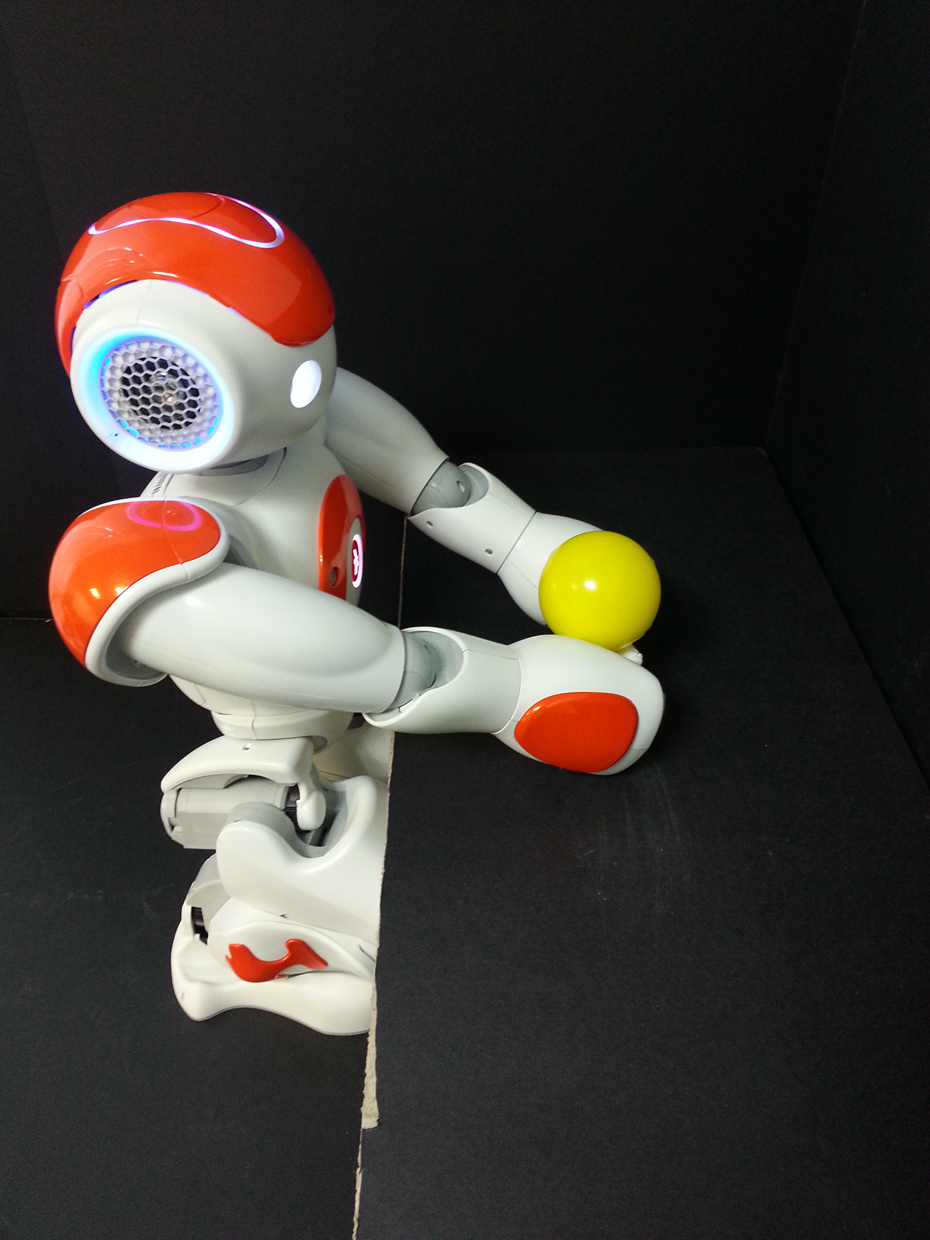
Ball lift.

Figure 6.

Ball roll.

Figure 7.

Bell ring left.

Figure 8.

Bell ring right.

Figure 9.

Ball roll on plate.

Figure 10.

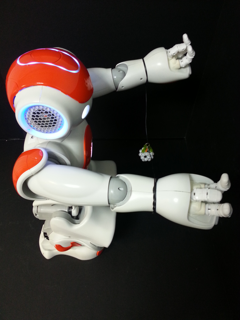
Ropeway.

For each of the six behaviors, we sampled 100 time steps of encoder values. These 100 time steps of values constitute one sequence. We repeated the sampling for 100 times, thus obtaining 100 sample sequences for one class of behavior. The same is repeated for all six behaviors. The encoder data were sampled at a sampling rate of f_s = 20 Hz.

At the end of the sampling, the samples for each behavior class can be represented as a single large matrix containing all the sample sequences. Formally, sampled behavior matrix B for one behavior class can be stated as a matrix containing column vectors of encoder values x(t) across time step, T. In our case, time step, T, is 100 for each sample sequence. The column vector, x(t), can be expressed as

x (t) = [\begin{array}{l} x_{1} (t) \\ x_{2} (t) \\ x_{3} (t) \\ x_{4} (t) \\ x_{5} (t) \\ x_{6} (t) \\ x_{7} (t) \\ x_{8} (t) \\ x_{9} (t) \\ x_{10} (t) \end{array}]

In other words, x(t) is a vector of the instantaneous encoder values from 10 specific joints at time, t . Thus, the behavior matrix, B can be expressed as

B = [\begin{matrix} x_{1} (1) & x_{1} (2) & .. & .. & x_{1} (T) \\ x_{2} (1) & x_{2} (2) & .. & .. & x_{2} (T) \\ x_{3} (1) & x_{3} (2) & .. & .. & x_{3} (T) \\ x_{4} (1) & x_{4} (2) & .. & .. & x_{4} (T) \\ x_{5} (1) & x_{5} (2) & .. & .. & x_{5} (T) \\ x_{6} (1) & x_{6} (2) & .. & .. & x_{6} (T) \\ x_{7} (1) & x_{7} (2) & .. & .. & x_{7} (T) \\ x_{8} (1) & x_{8} (2) & .. & .. & x_{8} (T) \\ x_{9} (1) & x_{9} (2) & .. & .. & x_{9} (T) \\ x_{10} (1) & x_{10} (2) & .. & .. & x_{10} (T) \end{matrix}]

We formed our data set of six behaviors based on the sampled data. Each sequence in each behavior is given an appropriate label for classification purposes. The data set are made available at the following site:

https://github.com/dnth/behavior-dataset

Network architectures

We evaluated several neural network architectures in this study in order to find an architecture that can perform best on the behavior classification task. The architecture of the evaluated networks are as follows:

LSTM with one hidden layer containing 20 LSTM memory cells. Recurrent connections are only allowed in the hidden layer.

Simple recurrent neural network (SRNN) with one hidden layer containing 44 neurons. Neurons in the hidden layers utilize the logistic sigmoid activation function. Recurrent connections are only allowed in the hidden layer.

TDNN with one hidden layer containing 25 neurons. The sliding time window, T, parameter is set to T = 10 time steps. Hidden neurons utilize the logistic sigmoid activation function. Our implementation of TDNN in this study is similar to the one of Noda et al.³⁴ with the usage of sliding time windows, T. More details of the TDNN can be found in the study by Kaiser³⁶ and Waibel et al.³⁷

MLP with one hidden layer containing 153 hidden neurons. Hidden neurons utilize the logistic sigmoid activation function. The implementation of MLP is similar to the study by Ciresan et al³⁸ albeit we limit our number of hidden layers to only one due to limited computational resources.

The number of neurons in the hidden layer was chosen such that all network models have approximately the same number of parameters in order to justify a fair comparison among different models. Table 2 shows the number of tunable parameters in each of the neural network model.

Table 2.

Total number of tunable parameters (weights and biases) of each network architecture.

Network	Total parameters
LSTM	2600
SRNN	2684
TDNN	2681
MLP	2607

LSTM: long short-term memory; SRNN: simple recurrent neural network; TDNN: time-delay neural network; MLP: multilayer perceptron.

During the training phase, we implement the early stopping training technique and L₂ (weight decay) regularization as a precaution against overfitting. The early stopping training technique is implemented as shown in algorithm 3.

The loss function, L, is stated as

L = \underset{\underset{MSE term}{⏟}}{\frac{1}{n} \sum_{i = 1}^{n} ∥ ({\hat{y}}_{i} - y_{i} {) ∥}^{2}} + \underset{\underset{⏟}{weight decay term}}{\frac{λ}{2} \sum_{i} w_{i}^{2}}

In equation (9), L is the loss function, n is the number of training samples, y is the targeted output, and $\hat{y}$ is the actual output by the model trained. The first term is known as the mean squared error term. The second term is also known as the weight decay term. The weight decay term is used to penalize large weights as a form of regularization to prevent overfitting of the models.^39,40 The training for all network is done by minimizing the formulated loss function L.

For the output neurons of all network models, we apply the Softmax function to estimate the probability of a sequence belonging to one of the six classes of behaviors. The Softmax function is given by

{\hat{y}}_{k} = \frac{e^{a_{k}}}{\sum_{k^{'} = 1}^{K} e^{a_{k^{'}}}}

where K is the total number of outputs and a_k is the weighted sum on the k -th node. The denominator is the normalization consisting of sum of exponentials over all output nodes ensuring that the output sums to 1. The Softmax function squashes the values of the hidden layer output in the range (0,1). Due to this property, the Softmax function is often used to estimate the probability of an event or action in a multiclass classification problem.⁴¹

Algorithm 1. Early stopping training algorithm.

0: count ← 0

1: while count < 100 do

2: Train network

3: if no improvement on validation set error then

4: count ← count + 1

5: end if

6: if improvement on validation set error then

7: count ← 0

8: end if

9: end while

Experiment and discussions

In this section, we present our experiment setup and results. The experiment setup is divided into two parts. The first part of the experiment explores the performance of the network models on the data set. In this experiment, we evaluate the recognition rate of the network models on the training, validation, and test set. In the second part of the experiment, we evaluate the same network models on a noise-robustness test. In this part of the experiment, we explore and investigate the networks in search for the model that is least influenced by noisy input data. The detailed procedures of the experiment setups will be elaborated in each respective subsection.

Performance on data set

In this experiment, we evaluate the classification accuracy performance of all network models on the data set. The evaluation is done on three separate portions of the data set, that is, the training set, validation set, and the test set. Evaluation is done by forward passing all sequences belonging to the data set and calculating its classification accuracy with respect to the true labels. Table 3 tabulates the classification accuracy of each model.

Table 3.

Classification accuracy performance of all network models on the training, validation and test set together with the number of weight parameters and training epochs.

Network	Total parameters	Training epochs	Training set (%)	Validation set (%)	Test set (%)
MLP	2607	632	100.00	100.00	99.71
TDNN	2681	364	100.00	100.00	99.92
SRNN	2684	426	99.99	99.71	99.88
LSTM	2600	168	100.00	100.00	100.00

MLP: multilayer perceptron; TDNN: time-delay neural network; SRNN: simple recurrent neural network; LSTM: long short-term memory.

In this experiment, all network models were ensured to have approximately the same number of parameters. Based on the classification results in Table 3, we observe that all models show almost on par performance on the classification accuracy. We observe that the MLP, TDNN, and the LSTM performed equally well on the training and validation sets. However, the performance on the test set differs for all models. The test set is not used during the training process. Hence, the sequences in the test set are new to all the models. By testing the models on new data, we can gauge how well the models are able to generalize on data they have not encountered before during training. We therefore take the performance of the models on the test set as the generalization performance of the network models. Based on the test set results, LSTM outperforms all other models that lead to a conclusion that the LSTM network is able to generalize better from the training and validation sets and performs best on the new data it has not encountered in the test set. As an additional advantage, compared to all models used in the experiment, the LSTM possesses the least number of weight parameters.

In this experiment, the result of the MLP network is taken as the baseline performance for all models. This is due to the fact that the MLP network does not take into consideration contextual information in a sequence, that is, the network treats every single point in the data set as independent and identically distributed (i.i.d.). Therefore, in theory, the performance of the MLP should be worse compared to other models that consider contextual information such as SRNN, TDNN, and LSTM. We observe in the classification results that, even without considering the contextual information, the MLP is able to score an impressive 99.71% on the test set. The impressive performance of the MLP suggests that even with discarded contextual information, the model is still able to differentiate different sequences by only looking at single data frame at a time. The impressive performance of the MLP may also be a result of relatively simple data set of behaviors that consists only of sequence that spans less than 100 time steps across. Also, the sequences that were used in this study involved repetitive movements, which may simplify the problem.

On the other hand, TDNN does not treat each point as i.i.d., rather, it considers an amount of contextual information based on a predefined time window value, T.⁴² In our implementation of the TDNN, we let the time window variable, T = 10. In the case of T = 10, the TDNN network will consider input data of the past 10 time steps in order to classify the behaviors. Data that lies outside the value of T will not be taken into consideration for classification. We observe that by taking into account the values of the past 10 time steps, the TDNN offers an improvement to the MLP score by scoring 99.92% on the test set. The performance of TDNN with T = 10 suggests that by taking into account temporal information from the past 10 time steps, the model is able to attain better results.

The SRNN differs from the MLP and the TDNN model in which the former is an RNN while the latter are both feedforward networks. In our implementation of RNN, we allow the network to only have recurrent connections in the hidden layer. Recurrent connections or recurrency in the RNN model allows the RNN to consider an amount of temporal information from previous time steps. However, there is no specific variable determining how many time steps to consider like in the case of TDNN, but rather the length of information to consider is automatically learned from the data during training. The concept of not having to specify specific knowledge pertaining to the behavior of the data is an added advantage for a general framework of behavior recognition because the number of time steps of contextual information may vary from one behavior to another. The network should be able to learn them from the data set. Predetermining the time window of contextual information as in the case of TDNN would impose limitations on the network to only suit certain behaviors well and would not suit behaviors that are longer than the time window. Our implementation of RNN is also known as the simple RNN or the Elman network in which the recurrent connection only occurs in the hidden layer. The RNN scored 99.88% of correct classification in the test set, a slight decrease in performance compared to the TDNN. We deduce that the slight decrease in performance can be caused by a known problem in RNN, the vanishing gradient problem.⁴³ The vanishing gradient is a known problem in RNN in which it does not allow the RNN to remember inputs from the far past. In a report by Graves,¹¹ the author documented that the RNN is limited to remembering approximately 10 time steps of past inputs. Information further away in the past is overwritten by more recent ones. This is a great disadvantage in behavior recognition task as it will not enable the RNN to learn longer behaviors with long-term dependencies.

However, the LSTM network is designed to remedy the problem of vanishing gradient in RNN. LSTM as proposed by Hochreiter and Schmidhuber¹⁰ replaces the normal sigmoid units in RNN with memory units. These memory units enable the LSTM networks to learn long-term dependencies that exist in the case of longer sequences. In our implementation of the LSTM network, it scored 100.00% on the test set of short and primitive behavior classification. LSTM also proved to be easier to train⁴⁴ compared to the RNN in which LSTM networks converged faster compared to all other models with approximately the same number of weights. The advantages of the LSTM model compared to all other models used in this experiment lead us to believe that the LSTM model is superior in classification accuracy performance when compared to MLP, TDNN, and RNN models.

In this section, we conclude that we can approach the task of primitive behavior recognition of simple, repetitive sequences with reasonable accuracy without using models that have advantage of capturing temporal dependencies such as RNN, TDNN, and LSTM. However, in terms of classification accuracy and generalization, LSTM is still superior to other models by a small margin.

We had also implemented algorithm that obtained the best classification on the data set (LSTM model) to classify behaviors of the NAO humanoid robot in real time. In the test, we sequentially demonstrate a sequence of behaviors on the robot in the following order: ball lift > ball roll > bell ring left > bell ring right > ball roll on plate > ropeway and have the LSTM network classify these sequences. Illustrated in Figure 11 is the result of the classification with respect to time.

Figure 11.

Real-time behavior classification on the NAO robot using the LSTM. LSTM: long short-term memory.

Noise robustness

In this experiment, we evaluated the noise robustness of all the trained neural network models by subjecting the input sequences to random Gaussian noise and measuring the performance of the models by monitoring the recognition rate. The equation of the Gaussian is given by

p_{G} (z) = \frac{1}{σ \sqrt{2 π}} e^{- \frac{{(z - μ)}^{2}}{2 σ^{2}}}

where p corresponds to the probability density function of a Gaussian random variable z, μ is the mean, and σ is the standard deviation.

All the sequences used in this experiment belong to the test set that is not used during training. The test set consisted of 120 sequences, each spans across 100 time steps. Before imposing noise on the test set sequences, we performed an initial test on the sequences with no noise. The test was carried out in 30 repeated trials. During each trial, the sequences were randomly picked. Next, we superimposed Gaussian noise with μ = 0 and σ = 0.1 onto the test set sequences and plotted the recognition rate in 30 repeated trials. The experiment was repeated with σ = 0.2, 0.3, 0.4 up to σ = 2.0. Figure 12 shows the performance of each network model when the sequences were corrupted by Gaussian noise.

Figure 12.

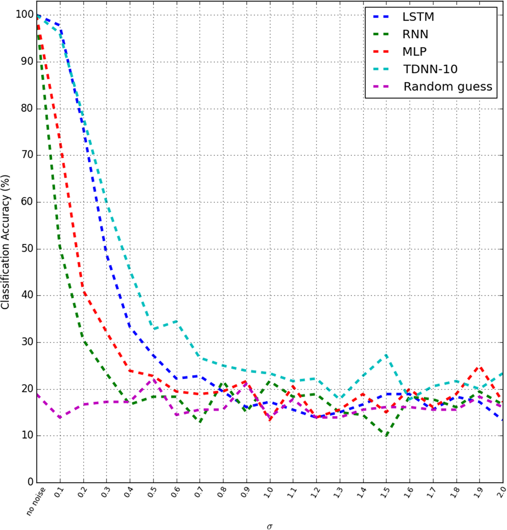
Performance comparison of all network models when the input is subjected to Gaussian noise. The standard deviation error bar is omitted for clarity.

We observe that without any presence of noise, all four network models appear to have on-par performance of perfect score. Conversely, the performance of each model starts to degrade at different rates once Gaussian noise was superimposed on the test sequences.

Referring to Figure 12, we observe that from σ = 0.1 to σ = 0.3, LSTM and TDNN seem to be comparable at noise robustness performance. At σ = 0.1, the LSTM outperforms all models by scoring 97.77% accuracy compared to 96.11% accuracy of TDNN, 73.33% of MLP, and 50.55% of RNN.

As a baseline result, we included a random classifier that randomly picks (or guesses) the class of the sequences corrupted with noise. The average of the baseline score of the random classifier is at 16.40% average accuracy with 14.91% average standard deviation. Therefore, performance accuracy that goes lower than this saturation point is considered insignificant and can be said only-as-good-as-a-random-guess performance. With the presence of the saturation point, we are able to gauge the performance of the noise robustness test better by knowing the threshold of minimal performance.

We observe in Figure 12 that the model that is least influenced by noise is the TDNN model. The saturation point of the TDNN model is at σ = 1.3 with accuracy score 17.77% and 16.06% standard deviation. The RNN can be said as the model that is most sensitive to Gaussian noise by having classification accuracy score descend to about 16.66% with 15.51% standard deviation at Gaussian noise σ = 0.4. The MLP follows hereafter with 19.44% accuracy with 15.56% standard deviation at Gaussian noise σ = 0.6. Next, we observe that the LSTM model reaches saturation point at Gaussian noise σ = 0.8 by scoring 19.44% with standard deviation 15.56%. Table 4 tabulates the saturation point of each model and the accuracy and standard deviation at the saturation point. We conclude from this result showing that the TDNN is the most noise robust model followed by LSTM, MLP, and RNN models.

Table 4.

Saturation point of network models and the accuracy and standard deviation at saturation point.

Model	Saturation point	Accuracy (%)	Standard deviation (%)
MLP	σ = 0.6	19.44	15.56
TDNN	σ = 1.3	17.77	16.06
RNN	σ = 0.4	16.66	15.51
LSTM	σ = 0.8	19.44	15.56

MLP: multilayer perceptron; TDNN: time-delay neural network; SRNN: simple recurrent neural network; LSTM: long short-term memory.

On a side note, all the network models in this experiment are trained with the original data without any preprocessing and addition of noise in the training process. The noise robustness accuracy score can be further improved by injecting noise into the training data, a well-known technique to achieve better performance in neural networks.⁴⁵

Conclusion and future improvements

With regards to our findings, we conclude that the problem of primitive sequence behavior recognition task can be approached using models that do not capture long-term dependencies. The use of LSTM as a model that is capable to capture long-term dependencies does not make much difference compared to other models. The true potential of the LSTM network is also not being exploited. LSTM network can in theory remember inputs from any arbitrary time steps from the past. In the upcoming works, we will exploit this trait of the LSTM networks by constructing a data set that incorporates long-term dependencies and monitoring the performances of the same network models.

In relation to the most recent work³⁴ by Noda et al., the contribution of this study is to introduce the use of recurrent variant of deep neural networks (LSTM) that solves the need of manually tuning the sliding time window, T, hyperparameter. The value of T that dictates how for in the past should the network remember to make a decision on the current event is learned automatically from the data sequence itself. We showed that in a simple supervised learning scheme, the LSTM is able to perform well in recognizing basic sequences. Even though the performance of the recognition is almost on par with other feedforward nets, we believe it is largely due to the nature of the sequences that are repetitive and does not require any long-term memory to distinguish them. Even though the true potential of the LSTM is not leveraged in this sense, we found that the LSTM is more noise robust compared to other networks tested. Noise robustness is a very desirable feature in the use of behavior recognition because behavior sequences may vary easily.

There are limitations of the work that need to be addressed as part of our study in this writing. First, the joint values utilized in the experiments are only limited to 10 specific joints on both the arms of the NAO robot. There are remaining 15 joints on the NAO robot that are not utilized. Including all the joints on the NAO robot is the ultimate goal for this experiment and is proposed as upcoming future improvements. Second, we limited the sampling of the behavior to 20 Hz for the behavior used in this study. From the documentation of the NAO robot, the robot is capable of a much higher sampling rate of 100 Hz. Third, we did not investigate into the execution time of the behavior sequence. We sampled all behaviors in consistent execution time in our study. The effects of drastically different execution time on the results are not known. Finally, even though all network models seem to obtain good classification result on the data set used in this study, the models are not tested against other public data sets to verify the robustness of the proposed framework.

Footnotes

Declaration of conflicting interests

The author(s) declared no potential conflicts of interest with respect to the research, authorship, and/or publication of this article.

Funding

The author(s) received no financial support for the research, authorship, and/or publication of this article.

References

Billing

Hellström

. Behavior recognition for segmentation of demonstrated tasks. In: IEEE SMC international conference on Distributed Human-Machine Systems 2008, 2008, pp. 228–234. Athens.

Pook

Ballard

. Recognizing teleoperated manipulations. In: Proceedings of the IEEE international conference on robotics and automation, 1993, pp 578–585. IEEE, 1993.

Urbanek

Albu-Schäffer

van der Smagt

. Learning from demonstration: repetitive movements for autonomous service robotics. In: Proceedings of the IEEE/RSJ international conference on intelligent robots and systems, 2004 (IROS 2004), Vol. 4, pp. 3495–3500. IEEE.

Hafner

Bachmann

. Human-humanoid walking gait recognition. In: 8th IEEE-RAS international conference on humanoid robots, 2008. Humanoids 2008, pp. 598–602. IEEE, 2008.

Nao companion robot, aldebaran robotics. Available at: https://www.aldebaran.com/en/humanoid-robot/nao-robot, 2016 (accessed 26 January 2016).

Huang

Lee

Learned-Miller

. Learning hierarchical representations for face verification with convolutional deep belief networks. In: IEEE conference on computer vision and pattern recognition (CVPR), pp. 2518–2525. IEEE, 2012.

Krizhevsky

Sutskever

Hinton

. Imagenet classification with deep convolutional neural networks. In: Advances in neural information processing systems, 2012, pp. 1097–1105. Nips Foundation.

Zhang

Ren

. Deep residual learning for image recognition. arXiv preprint arXiv:1512.03385, 2015.

Amodei

Anubhai

Battenberg

. Deep speech 2: end-to-end speech recognition in English and Mandarin. arXiv preprint arXiv:1512.02595, 2015.

10.

Hochreiter

Schmidhuber

. Long short-term memory. Neural Comput 1997; 9(8): 1735–1780.

11.

Graves

Neural networks. In: Graves

(ed.) Supervised Sequence Labelling with Recurrent Neural Networks. Berlin Heidelberg: Springer, 2012, pp. 15–35.

12.

Greff

Srivastava

Koutník

. LSTM: a search space odyssey. arXiv preprint arXiv:1503.04069, 2015.

13.

Doetsch

Kozielski

Ney

. Fast and robust training of recurrent neural networks for offline handwriting recognition. In: 14th International conference on frontiers in handwriting recognition (ICFHR), 2014, pp. 279–284. IEEE.

14.

Zaremba

Sutskever

Vinyals

. Recurrent neural network regularization. arXiv preprint arXiv:1409.2329, 2014.

15.

Luong

Sutskever

. Addressing the rare word problem in neural machine translation. arXiv preprint arXiv:1410.8206, 2014.

16.

Sak

Senior

Beaufays

. Long short-term memory based recurrent neural network architectures for large vocabulary speech recognition. arXiv preprint arXiv:1402.1128, 2014.

17.

Fan

Qian

Xie

. TTS synthesis with bidirectional LSTM based recurrent neural networks. In: Interspeech, pp. 1964–1968, 2014.

18.

Sønderby

Winther

. Protein secondary structure prediction with long short term memory networks. arXiv preprint arXiv:1412.7828, 2014.

19.

Marchi

Ferroni

Eyben

. Multi-resolution linear prediction based features for audio onset detection with bidirectional LSTM neural networks. In: IEEE international conference on acoustics, speech and signal processing (ICASSP), 2014, pp. 2164–2168. IEEE.

20.

Donahue

Hendricks

Guadarrama

. Long-term recurrent convolutional networks for visual recognition and description. In: Proceedings of the IEEE conference on computer vision and pattern recognition, 2015, pp. 2625–2634. IEEE.

21.

Peters

Campbell

Bluethmann

. Robonaut task learning through teleoperation. In: Proceedings of the IEEE international conference on robotics and automation (ICRA’03), Vol. 2, 2003, pp. 2806–2811. IEEE.

22.

Koenig

Mataric

. Behavior-based segmentation of demonstrated tasks. In: Proceedings of the international conference on development and learning, SAGE, 2006.

23.

Fod

Matarić

Jenkins

. Automated derivation of primitives for movement classification. Autonom Robots 2002; 12(l): 39–54.

24.

Nakaoka

Nakazawa

Yokoi

. Recognition and generation of leg primitive motions for dance imitation by a humanoid robot. In: Proceedings of 2nd international symposium on adaptive motion of animals and machines, Kyoto, Japan, 4–8 March 2003.

25.

Nicolescu

MN.

A framework for learning from demonstration, generalization and practice in human-robot domains. PhD Thesis, University of Southern California, USA, 2003.

26.

Ardizzone

Chella

Pirrone

. Pose classification using support vector machines. In: Proceedings of the IEEE-INNS-ENNS international joint conference on neural networks, 2000 (IJCNN 2000), Vol. 6, 2000, pp. 317–322. IEEE.

27.

Bentivegna

. Learning from observation using primitives. PhD Thesis, Citeseer: Georgia Institute of Technology, 2004.

28.

Kohonen

Learning vector quantization. Berlin, Heidelberg: Springer, 1997.

29.

Park

Kim

Jang

. HMM-based gesture recognition for robot control. In: Marques

de la Blanca

Pina

(eds) Pattern recognition and image analysis. Berlin, Heidelberg: Springer, 2005, pp. 607–614.

30.

Billing

Hellström

. A formalism for learning from demonstration. Paladyn J Behav Robot 2010; 1(1): 1–13.

31.

Rohrer

Hulet

. A brain emulating cognition and control architecture. Progr Biol Cybernet Res 2008: 1, https://books.google.com.my/books?hl=en&lr=&id=amcFw2fQuPwC&oi=fnd&pg=PA1&dq=a+brain+emulating+cognition+and+control+architecture&ots=9HuKOk86uN&sig=38PMfkZnQ6eAnpyuOUorkFEhH_E&redir_esc=y#v=onepage&q=a%20brain%20emulating%20cognition%20and%20control%20architecture&f=false.

32.

Rohrer

Hulet

. A learning and control approach based on the human neuromotor system. In: The first IEEE/RAS-EMBS international conference on biomedical robotics and biomechatronics, 2006. BioRob 2006, 2006, pp. 57–61. IEEE.

33.

Chalodhorn

MacDorman

KF,

Asada

. Humanoid robot motion recognition and reproduction. Adv Robot 2009; 23(3): 349–366.

34.

Noda

Arie

Suga

. Multimodal integration learning of robot behavior using deep neural networks. Robot Autonom Syst 2014; 62(6): 721–736.

35.

Noda

Arie

Suga

. Multimodal integration learning of object manipulation behaviors using deep neural networks. In: 2013 IEEE/RSJ international conference on intelligent robots and systems (IROS), 2013, pp. 1728–1733. IEEE.

36.

Kaiser

. Time-delay neural networks for control. In: Proceedings of the symposium on robot control, Vol. 94, 1994.

37.

Waibel

Hanazawa

Hinton

. Phoneme recognition using time-delay neural networks. Acoust Speech Signal Proc IEEE Trans 1989; 37(3): 328–339.

38.

Ciresan

Meier

Gambardella

. Deep, big, simple neural nets for handwritten digit recognition. Neural Comput 2010; 22(12): 3207–3220.

39.

Moody

Hanson

Krogh

. A simple weight decay can improve generalization. Adv Neural Inform Proc Syst 1995; 4: 950–957.

40.

Krogh

Hertz

JA.

A simple weight decay can improve generalization. Moody

Hanson

Lippmann

(eds), Technical Report no. P00002313, Nips Foundation, 1992.

41.

Bishop

. Pattern recognition and machine learning, Vol. 1. New York: Springer, 2006.

42.

Lang

Waibel

AH,

Hinton

. A time-delay neural network architecture for isolated word recognition. Neural Netw 1990; 3(l): 23–43.

43.

Hochreiter

Bengio

Frasconi

. Gradient flow in recurrent nets: the difficulty of learning long-term dependencies, 2001.

44.

Sutskever

Vinyals

. Sequence to sequence learning with neural networks. In: Ghahramani

Welling

Cortes

Lawrence

Weinberger

(eds) Advances in neural information processing systems, 2014, pp. 3104–3112. Nips Foundation.

45.

. The effects of adding noise during backpropagation training on a generalization performance. Neural Comput 1996; 8(3): 643–674.

Behavior recognition for humanoid robots using long short-term memory

Abstract

Keywords

Introduction

Learning from demonstration

Neural networks in behavior recognition task

Long short-term memory

Related works

Methodology

Data collection

Network architectures

Experiment and discussions

Performance on data set

Noise robustness

Conclusion and future improvements

Footnotes

Declaration of conflicting interests

Funding

References