
Abstract
Flexible manufacturing based on rapidly reconfigurable robotic systems will enable factories to meet time-sensitive and fast-changing industrial demands. However, with the rise of modular systems there is also the need to quickly and easily determine which configuration is optimal for performing a certain task. In this article, we present a path-based ad hoc technique for determining the inverse and forward kinematics map based on relative joint space variable to reduce the computational complexity. The proposed technique is nonsingular and suits kinematic analysis and optimization of robotic systems with undetermined configuration, and it can be extended to solve generalized inverse kinematic of robotics system involving large number of joint variable.
Introduction
In the ever-changing world of technology, electronic products are continually becoming smaller and smaller, implying the need for the micromanufacturing of system components. The microfactory is an industrial robotic setup that allows for the quick changing of a factory’s layout to meet the changing needs of industry. 1 –3 It is popular to use modular components for the construction of robots, as modular components tend to be independent agents, making them amenable to relocation within the robotic infrastructure. 4 While downsizing for the purpose of micromanufacturing and modularizing joints for quick reconfigurability, designers must keep in mind the main concerns of the micromanufacturing industry, that is, the research of minimal actuations factory parts and fabrication accuracy.
The fabrication process in an automated manufacturing setting is normally a set of commands given by a central processing unit to a robotic manipulator to follow a certain trajectory. Therefore, the path that a manipulator must take in Cartesian space is often known before a specific robotic manipulator is designed. At this stage, the problem of fabrication comes down to selecting a configuration of prismatic and rotary robotic links that will minimize path error and also minimize the amount of space and time needed to complete the task. The most common way to obtain the joint angles needed for a robotic system is to solve kinematic problem. The approach can be applied when both the path and the robotic manipulator are known.
The determination of configuration using inverse kinematic is a method widely used in biomechanics for the analysis of human motion. For example, inverse kinematic analysis may be used to reconstruct anatomical parameters during some motor tasks such as handwriting or upper limb motor strategies. Vimercati et al. 5 observed that participants with Down syndrome tend to draw faster but with less accuracy, or that the motor sequence adopted in a pointing and tapping task may be also affected by the pathology. 6 Sale et al. 7 adopted an end effector-based robot to control the kinematics of the lower limb in patients with Parkinson’s disease in order to improve their mobility. Another example is the work of Ancillao et al. 8 who developed a protocol to reconstruct the kinematics of the upper limb and upper body during a drawing/handwriting task.
At the qualitative level, previous work in determining configurations for robotic and kinematic tasks has taken an agent-based approach, where each link is an agent and the objective is to coordinate the behaviors of all agents. For example, in 1996, Carnegie Mellon University’s Robotics Institute began a program called the Agile Assembly Architecture, whose purpose was to create an Internet interface through which users could input which robotic components they desired to use; a decentralized cooperative framework enabled each component to be modular, and thus allowed the system to be easily reconfigurable, while maintaining high operability. 9 –12 In similar work by Chen, 13 the tools for developing a reconfigurable robotic workcell were considered (with a workcell being a specific system component or robot). A model for automatic robot generation was presented, which was modular and geometry independent. Optimization of the robotic workcell was specified, and a communication and control framework presented for coordination among the system workcells, with the end goal being a CAD-like program that would enable the appropriate robotic configuration to be determined for a specific task. 13
At the quantitative level, Barraquand et al. 14 presented a robot path-planning method to handle high degrees of freedom (DOFs). In their method, a graph of the local minima of a potential function was constructed incrementally during the search for the goal configuration. Their method relied on numerical methods for a solution. Optimization from a slightly different approach was carried out by Snyman and Berner 15 who optimized over robotic parameters (link lengths, masses, etc.) rather than positions.
Other work includes the development of inverse kinematic mappings for “hyper-redundant” robots. In the study by Chirikjian, 16 the author presents a “backbone curve” technique to compare manipulator configurations. Goldenberg et al. 17 present a technique based on the Newton–Raphson numerical method to iteratively find an inverse kinematic mapping of a kinematically redundant robot. On the other hand, one work that closely addresses accuracy concerns is that by Park and Bobrow, 18 in which the authors develop methods for optimizing robotic configurations via the “rigid body guidance problem.” Fault tolerance, that is, trajectory planning that takes into account the failure of a joint, was proposed by Paredis and Khosla. 19 The authors discussed that added redundancy in the form of multiple actuators and joints can aid the robot in completing a task. Their most important point was that certain joint configurations make it difficult to use the manipulator.
In recent years, neural network-based technique has found various applications for inverse kinematics. 20 The work by Li et al. 21 proposes a strategy with hierarchical tree generation on topology and nonlinear neural dynamics to control multiple manipulator with only partial command. The method is globally stable and the optimality is guaranteed, which makes it scalable to large number and types of manipulators including redundant DOF system. To solve redundant manipulator under physical constraints, Zhang et al. 22 proposed an online approach based on quadratic programming problem formulation for manipulator torque optimization using various levels of acceleration and velocity schemes.
Another approach to solving the inverse kinematics problem for redundant robots was given by Tabandeh et al., 23 who used a genetic algorithm to solve the inverse kinematics problem for a redundant robot by way of a niching method. They also used a numerical inverse kinematics solver to attain arbitrary accuracies of joint angles. Work by Chen2 and Chen and Yang, 24 addresses and solves the inverse kinematics problem for redundant serial and tree-type modular robots. Assuming that each link has only 1-DOF, is symmetric to all other links, the Jacobian is used to solve differential kinematics equations for the joint angles using the Newton–Raphson method. The work by Pac et al. 25 uses interval analysis in inverse kinematics problem to provide a range of joint space variables for a desired end effector position. Wu et al. 26 describe a rooted tree in module-level approach to generate kinematics of modular robots based on task-oriented concepts.
Meredith and Maddock 27 describe four different types of inverse kinematic mappings, one of which is called the analytical method; analytical methods are described as those that “reduce the inverse kinematics problem to a mathematical equation that need only be evaluated in a single step to produce a result.” 27 One of the drawbacks of analytical methods is that they are often not scalable enough to handle large chains of integrators. 27 In many robotics applications, particularly in the case of a modular robot, it is economically efficient to determine the robotic configuration that will be the best for a certain task from an existing pool of components. For a system with many links, determining an inverse kinematic mapping for each possible configuration is time consuming, and limiting to the time-sensitive efficiency of many factories. Thus, an inverse kinematic mapping that can be applied to many different configurations of robotic components is needed. Given a path, a global definition of the translation and rotation necessary to move from one point to another must be reiterated in terms of the joint variables and joint limits.
Many of the concerns for modular robotic systems have been addressed in the literature, particularly in developing globalized inverse kinematic maps whose coordinates can be mapped to various robotic structures. In addition, many continuous inverse kinematic problems based on linearization method have been addressed in literature to compute a configuration of a manipulator capable of producing a prescribed trajectory in the task space. 28 –30 However, much of this work relies on the Homotopy technique or Newton-Raphson method, whose success depends on how close the initial guess of the solution is to the actual solution. 31 For initial guesses that are close to the actual solution, the run time of the algorithm is low, and Newton–Raphson techniques are ideal. For large joint displacements over small periods of time, in which smaller sampling intervals must be considered to maintain reasonable initial guesses for Newton–Raphson, computational complexity will increase.
Research aim
The first goal of this work is to present an algorithm that estimates the amount of rotation and translation needed to traverse a planar path using the path’s geometry. The second goal of this work is to outline a mapping scheme from a simplified robot to an actual 6-DOF manipulator, and then compare the manipulator’s performance for different configurations.
The contribution of this article is to present a framework in which the joint angles may be retrieved for motion along planar paths in Cartesian coordinates. This method is different from previously derived inverse kinematics methods in that no knowledge of the robot’s structure is needed to determine the joint angles. The method used is a non-gradient-based optimization problem that focuses on changes in the joint angles rather than the actual joint angles of the robots at each point during the task. Since these coordinates may be mapped to the workspace of any robotic configuration, this framework is ideal for reconfigurable robots. The contribution is also to compare the performance of a more complicated robotic arm to a simplified system, enabling the fast determination of manipulator efficiency along a path.
This article is organized as follows: we present the materials and methods in the “Materials and methods” section. We introduce inverse kinematic mapping to find joint angles along a path. Then, we introduce a simple robot with four links, which is used to implement an existing inverse kinematics algorithm. Then, we map the joint angles from the inverse kinematics map to a physical robot by introducing constraint equations. We present the results and discussion in the “Results and discussion” section. In this section, we discuss simulation results highlighting the use of the inverse kinematic map and the results of mapping joint angles to a physical robot. Finally, in the “Conclusion” section, we offer concluding remarks and discuss future directions for research.
Materials and methods
Path-based determination of the inverse kinematic map
The inverse kinematic mapping of a robot—serial, parallel, and mixed—is based on a method that involves approximating the curve by sampling points along the curve, and using the joint center of gravity and the vectors between two consecutive path points to obtain translation and rotation of the joint. For consecutive movement increments, the amount of rotation and translation is divided among the joints in proportion with the total amount of movement the joint is capable of. Suppose we have a path

where


Projections of the center of mass on a hemisphere, with
Notice that to solve this equation, two quantities must be specified: the translational joint angles, given by
Translation of the end effector
Suppose that between every consecutive pair of points p and q there is a straight line

If we let d to be the distance from the path to the center of mass of the final link, then
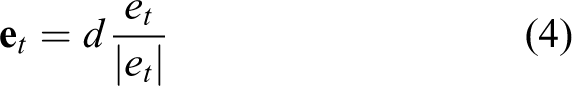
We assume that

Theorem 1
Recall that the translation of the mth link’s center of mass is given by

Proof. In appendix 1
The results of this proof indicate that using a large number of data points enhances the accuracy of the inverse kinematic mapping. On the other hand, the number of data points is proportional to the amount of time taken for the robot to complete the path. If we let the time needed to compute a single data point be

Thus, although smaller time increments increase accuracy, they also increase the run time of the robot along the path. The engineer must balance throughput with accuracy by tweaking such parameters.□
Rotation of the end effector
For any given vector in
Since we have approximated the path with line segments between path-points, we may estimate the amount of rotation that the manipulator has undergone using the dot product between two consecutive end effector orientations

This gives us the amount of rotation in the plane formed by the two vectors
We measure the accuracy of the robot along the path by comparing the “fit” of the path generated from the inverse kinematics mapping—which is defined by a polygon that is passing through a set of vertices—to the original path, that is, we measure the Euclidean distance between points on the generated path and the corresponding points on the original path. Since error is cumulative, we compare performance at different path parcings by examining the average error per time increment. The error at time t is given by

where

Global joint angles from a simplified manipulator
In this section, we demonstrate the use of joint angles from an inverse kinematic map using a simple robot. We consider a robotic manipulator that consists of three linear joints: one that traverses the x direction, one that traverses the y direction, and one that traverses the z direction. It also consists of one rotary joint that is assumed to rotate about the local x- or z-axis. Such kind of robots essentially boil down to the inverse kinematics of a spherical dyad. The four links are shown in Figure 2. There are 64 configurations possible from these components, that is
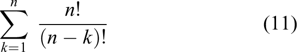
configurations possible from the four links, and we compare them based on average error and computational cost, where n is the original set of joints. For a given path we measure the error in the manipulator’s performance under the inverse kinematic map based on the equation (10).

The simple robot in the (1234) configuration shown in the top view and side view. Links 1, 2, and 3 are the x-, y-, and z-directional linear joints, respectively. Link 4 is the 2-DOF rotary joint. The white dot on link 4 is representative of an end effector.
We obtain the joint angles from the paths using the well-known Paden–Kahan subproblems produced by Murray et al.
32
Since there are essentially only two revolute joints, we determine joint angles using Paden–Kahan subproblem 2, featured. The joint angle trajectories are determined from the path by applying subproblem 2 repeatedly to consecutive points along the path. Again, let the first point sampled be denoted by

We find the vector,

The coefficients α, β, and γ are found by


and

Using

and

then the rotation may be found as

An identical procedure may be used to find
and

so that
we have that the translation is given by
Mapping joint angles to a physical system
The variables that we wish to find at each time step are the changes in the robot’s joint angles. The robot’s movement in 3-space can then be defined as
We also represent constraints on the revolute motion of the robot as

where m is the number of revolute variables affected by the constraint,
To determine the optimal solution angles based on minimum path error between time t and
By taking partial derivatives of the Lagrangian with respect to each variable and setting the resulting equations equal to zero, we have

With this framework, we are able to solve for each of the desired joint angles of the target robot.
Example using a 6-DOF manipulator
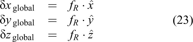
Inverse kinematics using the simplified robotic structure gives us global definitions of the amount of rotation about the x- and y-axes, and translation in all three directions. The next step is to map these globally referenced joint variables to the 6-DOF robotic manipulator. Unlike the simplified representation, only 6-DOF robot has rotary links.
To accomplish the mapping, we note that we have two rotational DOFs centered at the same center of rotation; during our comparison process, we sampled different configurations of the simplified robot, and moved the center of rotation to various positions within the robot’s structure. We were able to compare which rotation center produced the most accurate following of the three-dimensional (3-D) path. As can be seen from Figure 3, the manipulator has six joints like the center of rotation for the simplified robot, each successive pair of joints can rotate in about two directions. Thus, in the mapping process, we can choose which two joints we would like to be the center of rotation and assign the two rotational joint angles to that pair. For the remaining joint angles, a combination of the unused rotational DOFs would need to be used to produce the needed translational motion. Let


6-DOF robot. Joints that enable rotation about the local z-axis are denoted by the cylindrical prisms, while joints that enable rotation about the local x-axis are denoted by circles. 6-DOF: 6 degrees of freedom.
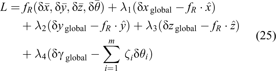
We now use constrained optimization to determine the remaining joint. The Lagrangian is given by

where

Suppose we choose joints 5 and 6 to be the center of rotation for the manipulator, and since joint 1 is at the base of the manipulator, we fix it so that it has zero rotation at all times. We can then reduce the size of the problem to one in which we have only three unknown joint angles to solve for. Thus, along with the Lagrange multipliers, the optimization variables we want to find are given by

The procedure for finding the core set of partial derivatives when the center of rotation is either links 3 and 4 or 1 and 2 is a similar process of removing those equations for the joint variables that are already known.
Equation (29) must be solved at every time step, and they have no closed form solution. Performing a Newton–Raphson technique at every time step could be computationally time consuming when path is discretized into very small step size. Thus, since we are taking small increments of movement and time, we linearize the equation (29) about the manipulator’s current pose, and solve the linearized system. Let “·” denote the dot product,
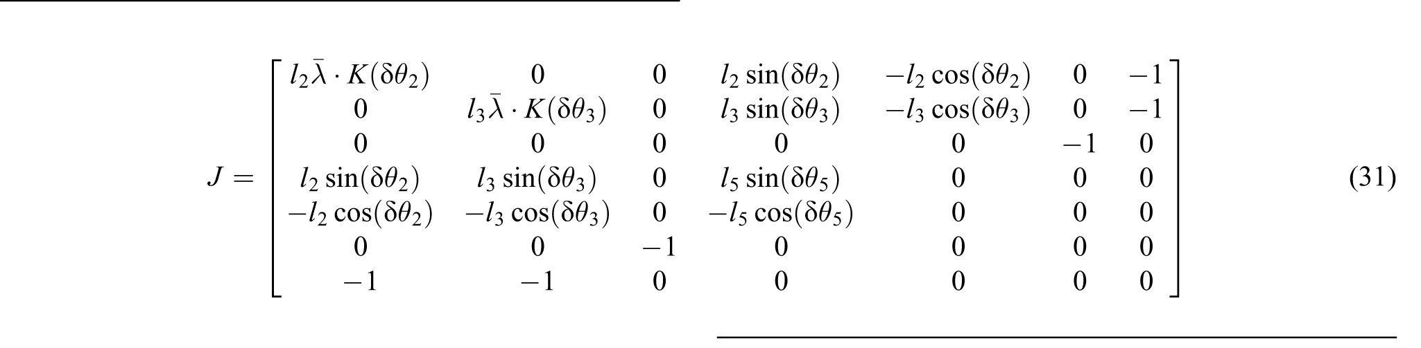
The linearized system is given by
Theorem 2
As the size of the state
Proof. In Appendix 2
For sufficiently small δθ, we can use the null space of the Jacobian matrix J to find the joint angles
Theorem 3
The Jacobian matrix J given by equation (31) is evaluated at the current value of the state δθ. That is
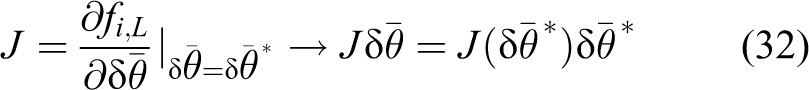
Therefore, the linearization is valid for arbitrarily large
Proof. In appendix 3
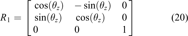
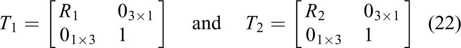
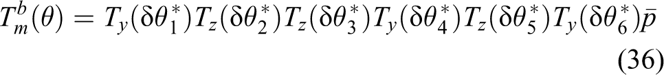
Upon finding the optimal joint angles, we substitute them into the forward kinematic map for the 6-DOF robot. If we let the matrix describing local rotations about the y-axis be given by

and the matrix describing local rotations about the z-axis be given by

and furthermore, let the center of mass of the i th link be given by

Thus, if
Since the system is linearized, using small time increments would be the most advantageous for increased accuracy along the path.□
Theorem 4
An optimal solution always exists for the system
Proof
Since any system
Transforming error of the simple robot to the 6-DOF manipulator
What if, given the average error per unit time of the simplified robot, we would like to predict the average error of the 6-DOF manipulator? Based on equation (13), we define the error measured by the simple robot to be

where

Let

Substituting equation (39) into equation (38) for

This transformation gives a mapping at time t from the error measured by the simple robot to the error measured by the 6-DOF manipulator. Since the transformations
Cost function
Different configurations have dissimilar path-following attributes that may make certain configurations more desirable than others. For instance, the more a linear joint moves along its DOFs, the more actuation is needed to produce the motion. Also, the heavier a joint, the more stress on the actuators to overcome the joint’s inertia. Finally, the most important factor—how well the robot, using the inverse kinematic map, follows the path, or the accuracy of the robot along the path—must be considered in a cost function. In this section, we focus on formulating a cost function that encapsulates all of these concepts in order to aid us in identifying which configuration has the most efficient behavior along a given path.
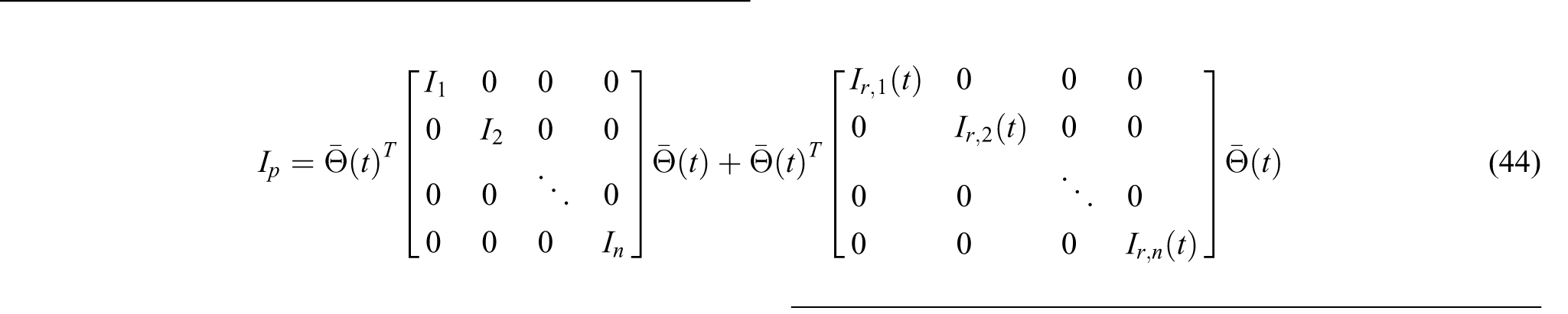
The cost function is composed of the joint variables, the inertia penalty, and the path error. We choose an energy-like cost function so that it will be amenable to control design. To obtain the cost, we use

where
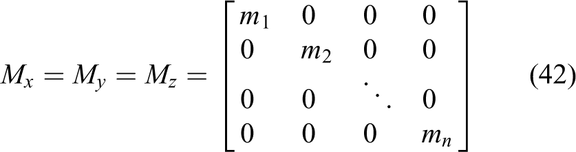
and

where


where E is the difference between the actual path

Results and discussion
In this section, we present the results of simulations using the proposed methodology for determining two-dimensional (2-D) path inverse kinematic maps, and for the case study of multiple configurations of a simplified robot whose joint angles have been mapped to a 6-DOF robotic arm. We implemented the algorithms in MATLAB (T. M. MATLAB 8.5, Inc., Natick, Massachusetts, United States). 6
2-D path generation along a planar sinusoid—error cost function
The planar path that we consider is given by

where
The results are shown in Figure 4, and confirm that smaller time increments—which correspond to small δθ increments in Theorem 3—produce higher accuracy between the generated curve and the curve produced using the output of the inverse kinematic map.

Tracing of a curved planar sinusoidal trajectory using the proposed inverse kinematic mapping. The time increments of
2-D path generation along a planar sinusoid—Generalized cost function
To test the inverse kinematic mapping, we use a three stages “joints” robot. Each slot is stacked vertically (along the y-direction). We have two linear joints, the first with one redundant DOF (x) and the other with two DOFs (x–z), and a rotary joint. We make the simplifying assumption that the rotary joint is a disk, and the two linear joints are rectangular plates as shown in Figure 5. We will use this system to test the inverse kinematic mapping along a sinusoid. The joint dimensions, movement capabilities, and slot information are shown in Table 1.
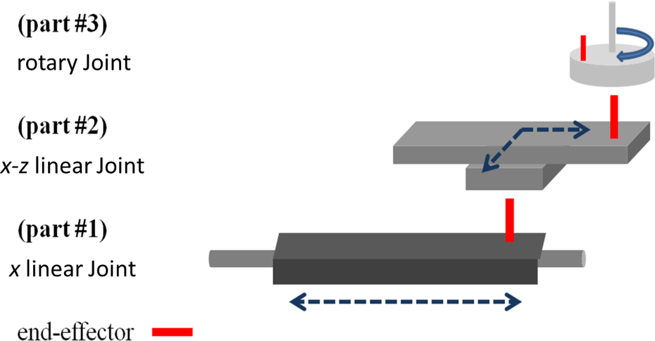
Physical representation of each stage “joint”.
Part and slot information.

For this exercise, we study the robot in the 1-2-3 configuration, whose forward kinematic mapping is given by
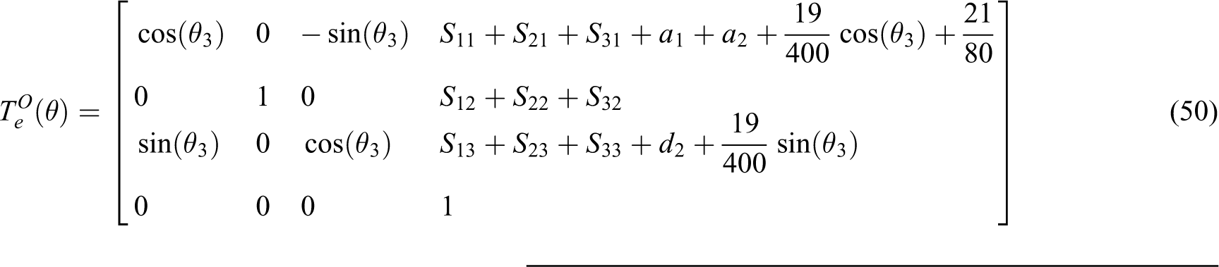
We can already see that for the selection of joint types and their slot orientations, the path of the end effector will always be planar, regardless of configuration.
The general equation for the sinusoid that we use is

where

where
Table 2 and Figure 6 compare the accuracy of the inverse kinematic map along the sinusoidal curve for increasing numbers of data points.
Comparison of accuracy with 10, 20, 40 and 100 data points.


(a) 40 data points and (b) 100 data points.
We use the 1-norm for comparison because using a single number allows us to quickly see the net effect of error over time. Taking the 1-norm of the difference between the desired and actual paths confirms that increasing the number of data points increases accuracy of the estimated path. Using the automatic-inverse kinematic map generation algorithm, we were able to compare n! configurations for the three-joint robot. The results are shown in Table 3.
Comparison of 1-norm of costs for all configurations when n = 3.

Under the chosen cost function, all of the six configurations that use all three joints have similar costs, while marked differences in cost can be seen for the six configurations that use only two of the joints and the three configurations that use only one of the joints. The reason for this pattern in the six configurations that use all three joints may be that regardless of the joint sequence, the same net movement is undertaken by the robot. This seems to indicate that the order in which parts are assembled does not matter, and could be due to the commutative nature of many of the joints involved and the fact that the approximate inverses always have a “trivial” unique solution. Increases in the inertia penalty due to configurations that place the rotary joint in either the first slot or the second slot are leveraged by smaller translations made by the joints. The “sweeping motion” of the rotary joint, particularly when the rotary joint is further in position from the path, eliminates much of the needed translation.
The costs for two-joint configurations is largely dependent on the joints being used. For instance, configuration 1-3 has a much lower cost than configuration 2-3 because 2-3 cannot traverse the entire sinusoid, and therefore accrues much more error than configuration 1-3. Configurations 1-2 and 2-1 actually have fairly low costs, even without the help of the rotary joint, because they are independently able to traverse the entire sinusoidal curve.
3-D path generation along a curved sinusoid
To test the efficiency of the various configurations of the simple robot, we consider using a curved sinusoid, given by the parametric representation

where

Schematic of simple robot with four groups of configurations.(a) Group of one rotational joint, (b) group of two rotational joints, (c) group of three rotational joints, and (d) group of four rotational joints.
Four groups of configurations for the simple robot based on the number of links. The time increment is

Depending on how the forward kinematics algorithms are implemented, matrix computations can be the most costly. Thus, the programmer must weigh the cost of production, judging between accuracy and computational efficiency.
The patterns in accuracy and computational efficiency of the simple robot can be extended to the 6-DOF manipulator when considered as separate cases. However, generating a correspondence relationship between the simple robot’s four links and the links of the 6-DOF manipulator is elusive at best, since several of the 6-DOF robot’s joint angles contribute to multiple global DOFs. To see an example of this, suppose that we set
Mapping error from the simple robot to the 6-DOF manipulator is more reliable. Using equation (40) and only considering the case when all four links of the simple robot and all six links of the 6-DOF robot are used, the results of the error mapping are shown in Figure 7. The inputs were the forward kinematic maps of the simple and 6-DOF robots, the error of the simple robot at time t, the end point

Comparison of path following given the original path
Conclusion
In this work, we have described a computationally efficient joint space algorithm that determines the configuration of a modular robotic system for a given path. We presented a framework in which the joint angles may be retrieved for motion along planar paths in Cartesian coordinates, where we reconstruct robot configurations using the change in the joint angles rather than the absolute values. To accomplish this, we first determine the inverse kinematic mapping based solely on the path traveled; then, applying the inverse kinematic map to all configurations of the robot, we compare each configuration based on accuracy in following the path, and minimal computation required. The developed algorithm allows users to input information about the joints of a robotic platform and receive an automatically generated forward kinematic mapping for any configuration of the joints, as well as the time-dependent joint variables along a given path. The generalized forward kinematic mapping can handle a set of distinct robotic joints as well as duplicate joints and still produce the appropriate mapping by the utilization of numerical part markers that the algorithm uses to query information about the joints considered. Using this inverse kinematic mapping has proven to render accurate reproductions of a path with bounded curvature and without singularity when the measured joint variables were placed through the forward kinematic mapping.
We also successfully map joint angles obtained from an existing 3-D inverse kinematics method to a physical 6DOF manipulator and set up the framework for comparing multiple configurations of this robot. Although such simple manipulator may have closed form solution, but our method is suitable for solving inverse kinematic of robotics system involving large number of joint variable, example may include self-assembly of molecular scale robots. This new comparison metric will enable designers and micro-machinists to build manufacturing platforms with prior knowledge of the configurations that produce the optimal output for the task, hence speeding up the rapid prototyping process significantly.
In future work, we will extend the two dimensional inverse kinematics scheme to three dimensions in order to completely specify a mechanism for the fast determination of optimal configurations in modular robotic platforms. We will also develop a cost function to more fully characterize the trade-off between computational efficiency and accuracy.
Footnotes
Acknowledgement
The authors would like to thank Dr Woo Ho Lee and Dr John Shin from the Robotics Division of the University of Texas at Arlington Research Institute for the valuable feedback. The authors declare that there is not conflict of interest that may have affected the outcomes of this work.
Declaration of conflicting interests
The author(s) declared no potential conflicts of interest with respect to the research, authorship, and/or publication of this article.
Funding
The author(s) disclosed receipt of the following financial support for the research, authorship, and/or publication of this article: This work was partially funded under a grant from Office of Naval Research.