Non-linear sliding mode control of the lower extremity exoskeleton based on human–robot cooperation

Abstract

This article presents a human–robot cooperation controller towards the lower extremity exoskeleton which aims to improve the tracking performance of the exoskeleton and reduce the human–robot interaction force. Radial basis function neural network is introduced to model the human–machine interaction which can better approximate the non-linear relationship than the general impedance model. A new method to calculate the inverse Jacobian matrix is presented. Compared to traditional damped least squares method, the novel method is proved to be able to avoid the orientation change of the velocity of the human–robot interaction point by the simulation result. This feature is very important in human–robot system. Then, an improved non-linear robust sliding mode controller is designed to promote the tracking performance considering system uncertainties and model errors, where a new non-linear integral sliding surface is given. The stability analysis of the proposed controller is performed using Lyapunov stability theory. Finally, the novel methods are applied to the swing leg control of the lower extremity exoskeleton, its effectiveness is validated by simulation and comparative experiments.

Introduction

Lower extremity exoskeleton is a special kind of man–machine interaction system which can combine the highly developed sensory, balancing, path planning capabilities of the wearer and the large payload capacity of the robot.^1,2 Obviously, it has numerous potential applications; for instance, it can help soldiers to walk or run with weights and it can provide accident rescue workers and other emergency personnel with the ability to carry heavy loads, such as rescue equipment, food and first-aid kit.^3,4 So exoskeletons have attracted great interests from many famous universities, military and the industry. The first energetically autonomous lower extremity exoskeleton (Berkeley lower extremity exoskeleton (BLEEX)) is designed to augment soldiers’ capability of carrying a heavy backpack.^5,6 Recently, a hybrid leg exoskeleton is designed to augment load-carrying by introducing novel Hy-Mo actuators. ⁷ A series of hybrid assistive leg (HAL) is developed to assist the hip and knee joint. ⁸ Raytheon has developed the second-generation exoskeleton called XOS2 for US Army. It can enhance the human strength, agility and endurance capabilities of the soldier in it. A research into a powered hip exoskeleton is presented and an anthropomorphic structure is designed with only six degrees of freedom. ⁹ In one word, a successful exoskeleton must be able to enhance the user’s strength and endurance and guarantee the agility and freedom of the user.

The effectiveness of the lower extremity exoskeleton depends on the control system’s ability to bring the wearer’s advantage of providing balance, navigation and path-planning into play while ensuring that the exoskeleton can support most of the payload.^10,11 So the exoskeleton needs to shadow the movement of the wearer in an intuitive and unobtrusive manner.^12,13 It also means to minimize the human–machine interaction force so that the wearer nearly can’t feel the existence of the exoskeleton and the payload. ¹⁴ The control of HAL is based on hybrid control method which used electromyography (EMG) sensors to measure human’s muscle biological information and generate the desired actuators control signals. ¹⁵ Sometimes the information from EMG sensors is not reliable and it is greatly influenced by the skin conditions where it is located. ¹⁶ A novel control scheme is executed in BLEEX which is called sensitivity amplification control. It needs no direct measurement from the human–machine interaction force, so it can eliminate the problems associated with measuring interaction forces or human muscle activity. However, it needs a very wide control bandwidth and has little robustness to parameter variations. ¹⁷ Another intuitive way of minimizing the human–machine interaction force is to measure the interaction force directly which is commonly used in upper-limb exoskeleton. ¹⁸ Lee got the generation of desired position of the exoskeleton by modelling human–robot interaction into virtual mechanical impedance. ¹⁹ Miranda adopted a spring to model the human–machine interaction and calculated the user’s intention. ²⁰ Considering the complexity and application of the human–machine model, Lee also proposed a Proportional-Integral (PI) model to infer the wearer’s movement intention.^19,21 Kwon utilized artificial neural network (NN) to approximate the non-linear relation between surface EMG and upper-limb motions. ¹³ The control system is very complicated which needs to get the signals from five upper-limb muscles and angular velocities of the limb joints.

In this article, radial basis function (RBF) NN is adopted to model the relationship between the force sensor and lower extremity exoskeleton which can approximate any continuous functions with approximate parameters.^22–24 Thus it can depict the non-linear relation of the human interaction in detail. When the exoskeleton approaches the kinematic singularity, the inverse Jacobian matrix becomes a singular matrix which makes the exoskeleton unstable and possibly causes an accident. A new method is proposed to solve the singularity problem with the pseudo-inverse Jacobian matrix which is more suitable for exoskeletons than damped least squares (DLSs). Finally, to ensure the swing leg of the exoskeleton shadows the wearer with minimal interaction force, an improved non-linear robust sliding mode control method is proposed and a new non-linear integral sliding surface is introduced to deal with the effect of parametric uncertainties and uncertainties of the system. Effectiveness of the proposed algorithms is verified by simulation and experiment.

A brief overview of the article is given as follows: in section ‘Architecture’, the lower extremity exoskeleton is introduced which is designed to aim the wearer to hold payload. In section ‘Human–robot interaction modelling’, RBF NN is recommended to model human–robot interaction in exoskeleton and is verified by simulation. In section ‘Swing leg modelling’, we proposed a new method to obtain the pseudo-inverse Jacobian matrix which is more suitable to apply in human–robot system and simulation has proved the result compared to other methods. In section ‘Controller design’, a novel non-linear sliding mode controller (INSM) with a non-linear integral sliding surface is proposed and the Lyapunov stability of the control law is proved. Finally, in section ‘Simulation experiment’, the comparative simulation and experiments are performed to verify the effectiveness of the proposed method. Section ‘Conclusion’ concludes this article.

Architecture

Human walking is a cyclic process that can be divided into stance phase and swing phase. Swing phase occupies approximately 40% of one cycle during the normal gait. ¹

The exoskeleton is shown in Figure 1 and consists of two anthropomorphic legs and a spine which is used to carry load. It belongs to pseudo-anthropomorphic architecture. This means although it has hip, knee and ankle joints like a human, the details of these joints are different from humans. ¹⁴ Overall, this lower extremity exoskeleton has seven distinct degrees of freedom per leg: three degrees of freedom at the hip, one degree of freedom at the knee and three degrees of freedom at the ankle. When the operator wears the exoskeleton, it will be attached at the feet, legs and upper body. According to some research studies, most of the power needed for walking is in the sagittal plane. So only the freedoms of hip and knee in sagittal plane are powered.^6,14

Figure 1.

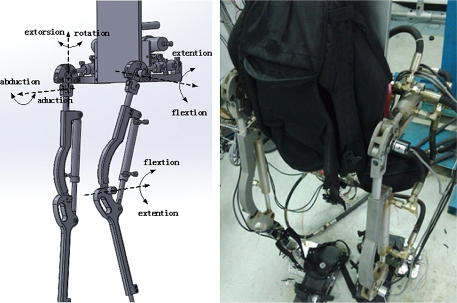
The lower extremity exoskeleton.

Human–robot interaction modelling

The first step to realize the aim actuating the swing leg to shadow the wearer synchronously is to get the wearer’s motion intention. It is identified using a six-axis force sensor mounted at the shank and encoders mounted at the joints. The swing leg tracks the motion intention so that the interface force converges to zero.

As shown in Figure 2, the exoskeleton is attached to the back, shank and feet of the wearer. Interaction force is generated by the connected shank interface. It also shows that human–robot interface is modelled using artificial NN which can approximate the non-linear relationship between interaction force and leg motions at any precision. ²⁵

Figure 2.

Human–robot interaction model using the RBF NN. RBF NN: radial basis function neural network.

RBF NN includes three feedforward layers. The network input terms are the interaction force and joint angles of hip and knee. The input vector is described as

$x={\left[\begin{array}{cccc}{\theta }_1& {\theta }_2& F_x& F_y\end{array}\right]}^T$

1

where θ₁ means the joint angle of hip in sagittal plane by angle encoder, θ₂ means the joint angle of knee in sagittal plane by angle encoder, F_x means the component force along shank and F_y means the component force whose direction is perpendicular to the shank.

The output terms are the angular velocities of knee and hip

$y={\left[\begin{array}{cc}{v}_x& v_y\end{array}\right]}^T=Wh$

2

where v_x means the velocity of the interaction point along the shank, v_y means the velocity of the interaction point whose direction is perpendicular to the shank, h is the output of hidden neurons and is described in equation (3) and W is the weight vector of the network which is described as $W=\left[\begin{array}{ccc}\begin{array}{ccc}{w}_{11}& \cdots & w_{1m}\end{array}& ;& \begin{array}{ccc}{w}_{21}& \cdots & w_{2m}\end{array}\end{array}\right]$ .

The number of hidden neurons is important to depict the non-linear relationship, so we tried to find the optimal number of hidden neurons based on the iterative method. The control algorithm of one hidden neuron can be described as

$h_j=\exp \left(-\frac{{\Vert x-c_j\Vert }^2}{2b_j^2}\right),j=1,2\mathrm{...}m$

3

where $h={[\begin{array}{ccc}{h}_1& \cdots & h_j\begin{array}{cc}\cdots & h_m\end{array}\end{array}]}^T$ and h_j is the Gaussian function and it means the output of the jth hidden neuron, $c_j=\left[\begin{array}{cccc}{c}_{j1}& c_{j2}& c_{j3}& c_{j4}\end{array}\right]$ means the jth centroid, $b=\left[\begin{array}{ccc}{b}_1& \cdots & b_m\end{array}\right]$ and b_j > 0 is the node-wide parameters of the node.

To evaluate the network, we defined a judgement function based on approximation error and variable parameters. It is described as

$E(t)=\frac{1}{2}\left[\alpha {\left(v_{xd}-v_x\right)}^2+\beta {\left(v_{yd}-v_y\right)}^2\right]$

4

where ${[\begin{array}{cc}{v}_{xd}& v_{yd}\end{array}]}^T$ is the desired velocity of the man–machine interaction point which is derived from equation (5), α,β ∈ [0, 1] are variable parameters which can be chosen based on which of the two velocities are more important.

${\left[\begin{array}{cc}{v}_{xd}& v_{yd}\end{array}\right]}^T=J·{\left[\begin{array}{cc}{\dot{\theta }}_1& {\dot{\theta }}_2\end{array}\right]}^T$

5

When the wearer moves the swing leg of the lower extremity exoskeleton, the input information of the RBF NN is stored based on related sensors. The MATLAB NN toolbox is used to train the network based on the stored information.

One thousand and eight hundred sampling input signals of the RBF NN are used to test the system, and another 200 sampling input signals are used to verify the trained neural system. Figure 3 shows the results, where (a) represents the obtained velocity by neural system compared to the real velocity and (b) represents the tracking error of the velocity. Obviously, it proves the mapping between the input vector x shown in equation (1) and velocities of human–machine interaction point is useful. Intuitively, the method is more accurate than impedance model in depicting non-linear relation.

Figure 3.

Simulation of the RBF NN. RBF NN: radial basis function neural network.

Accurate estimation of wearer’s motion intention generates accurate movement of the lower extremity exoskeleton, and it is a time-variant desired trajectory. Finally, the block diagram to control the lower extremity exoskeleton to shadow the wearer based on the human–machine cooperation is designed as shown in Figure 4.

Figure 4.

Block diagram of the control system for human–robot cooperation of the lower extremity exoskeleton.

Swing leg modelling

Although it is straightforward to obtain a model as a serial chain, closed-chain mechanisms are less intuitive and harder to analyse. A partitioned approach is used to analyse a closed-chain mechanism by deriving the dynamic model of the two separate parts. ²⁶ So we will focus on the swing leg which is also important to ensure the exoskeleton system shadow the operator in synchrony. It demands large degrees of joints movement and small human–robot interaction force.

The swing leg has similar degrees of freedom to those of the human body. Therefore, we set the joint coordinate systems in Figure 5, and the kinematics model is obtained based on the Denavit–Hartenberg parameter method.

Figure 5.

Coordination system, link parameters and DH parameters of the swing leg of the lower extremity exoskeleton. DH: Denavit–Hartenberg.

Based on the D-H parameters in Figure 5, the homogeneous transformation matrix is calculated in equation (6). Then, the Jacobian matrix is derived as shown in equation (7).

${}^0{T}_1=\left[\begin{array}{cccc}\begin{array}{c}\text{cos}{\theta }_1\\ \text{sin}{\theta }_1\\ 0\\ 0\end{array}& \begin{array}{c}-\text{sin}{\theta }_1\\ \text{cos}{\theta }_1\\ 0\\ 0\end{array}& \begin{array}{c}0\\ 0\\ 1\\ 0\end{array}& \begin{array}{c}{l}_1\text{cos}{\theta }_1\\ l_1\text{sin}{\theta }_1\\ 0\\ 1\end{array}\end{array}\right];{}^0{T}_2=\left[\begin{array}{cccc}\begin{array}{c}\text{cos}{\theta }_{12}\\ \text{sin}{\theta }_{12}\\ 0\\ 0\end{array}& \begin{array}{c}-\text{sin}{\theta }_{12}\\ \text{cos}{\theta }_{12}\\ 0\\ 0\end{array}& \begin{array}{c}0\\ 0\\ 1\\ 0\end{array}& \begin{array}{c}{l}_2\text{cos}{\theta }_{12}+l_1\text{cos}{\theta }_1\\ l_2\text{sin}{\theta }_{12}+l_1\text{sin}{\theta }_1\\ 0\\ 1\end{array}\end{array}\right]$

6

$J=\frac{\partial \Phi }{\partial \Theta }=\left[\begin{array}{ccc}\frac{\partial p_1}{\partial {\theta }_1}& \cdots & \frac{\partial p_1}{\partial {\theta }_n}\\ ⋮& \ddots & ⋮\\ \frac{\partial p_n}{\partial {\theta }_1}& \cdots & \frac{\partial p_n}{\partial {\theta }_n}\end{array}\right]=\left[\begin{array}{cc}-l_{2}s{\theta }_{12}-l_{1}s{\theta }_1& -l_{2}s{\theta }_{12}\\ l_{2}c{\theta }_{12}+l_{1}c{\theta }_1& l_{2}c{\theta }_{12}\end{array}\right]$

7

where ${\theta }_{12}={\theta }_1+{\theta }_2;s\theta =\text{sin}\theta ;c\theta =\text{cos}\theta$ .

As shown in Figure 5, when the swing leg reaches the kinematic regularity, the inverse Jacobian matrix becomes singular, which causes the system to be unstable. In this case, it’s dangerous for the wearer because the exoskeleton may vibrate and collide. So DLS method is adopted to avoid this problem in upper-limb exoskeleton.^19,27 The DLS method is described in equation

$\dot{\theta }=J^{†}v$

8

where $J^{†}=J^T{\left(J{J}^T+{\alpha }^{2}I\right)}^{-1}$ means the pseudo-inverse Jacobian matrix, I means an identity matrix and α is a non-zero real number.

To evaluate the effect of the DLS method used in lower extremity exoskeleton, we designed a simulation as follows

${\dot{\theta }}_1=J^{†}v$

9

$\dot{\theta }=J^{-1}v$

10

where ${\dot{\theta }}_1={\left[\begin{array}{cc}{\dot{\theta }}_{11}& {\dot{\theta }}_{21}\end{array}\right]}^T$ means the joint angular velocity calculated by the DLS method corresponding to the terminal velocity in operational space. $\dot{\theta }={\left[\begin{array}{cc}{\dot{\theta }}_1& {\dot{\theta }}_2\end{array}\right]}^T$ means the real joint angular velocity corresponding to the same terminal velocity.

Through Figure 6, where ω ₁ represents the angular velocity of the hip joint and ω ₂ represents the angular velocity of the knee joint, the DLS method really decreases the angular velocity of the joints with the factor α.

${\dot{v}}_1=J{\dot{\theta }}_1$

11

where v₁ means the terminal velocity in operational space corresponding to ${\dot{\theta }}_1$ . Two evaluation indexes are designed as follows

• the norm ratio of the vector v₁ and v: $k=\frac{\left|v_1\right|}{\left|v\right|}$

• the vector angle difference between v₁ and v: $\gamma =\arcsin \left(\frac{v_1\times v}{\left(\left|v_1\right|·\left|v\right|\right)}\right)$

Figure 6.

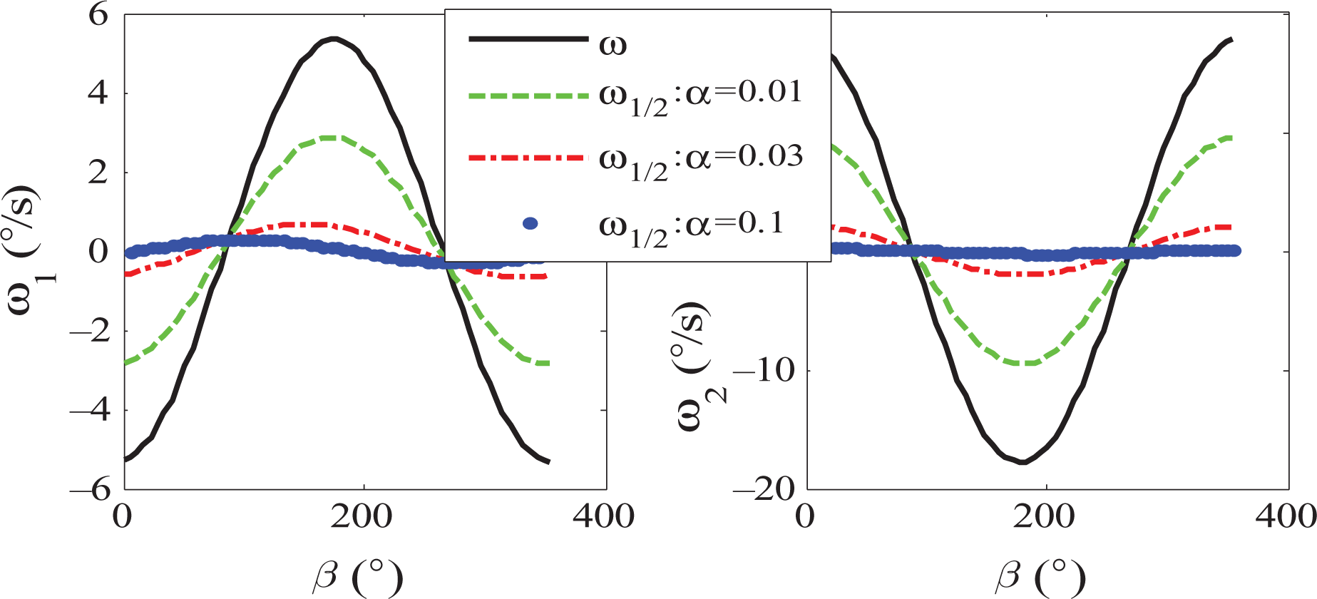
Angular velocity in joint space by the DLS method.

We suppose the parameters value as follows: θ₁ = 0°, θ₂ = −5° and the terminal velocity in operational space $\dot{v}=\left(\begin{array}{cc}0.2\text{cos}\beta & 0.2\text{sin}\beta \end{array}\right),\left(\beta \in \left[0,2\pi \right]\right)$ .

When we set the origin of the velocity vector in the same point and connect the terminal point of the vector, Figure 7 is plotted. It is obvious to show the real velocity differs from the calculated velocities by DLS method in amplitude and orientation. To justify the variation, we have defined two evaluation indexes and Figure 7 exhibits the norm ration and vector angle difference between the velocities. Obviously, the minimal value of k decreases and the maximal value of γ increases as α increases.

Figure 7.

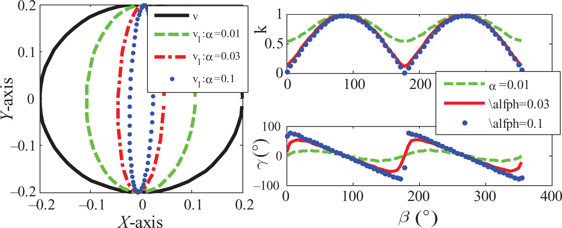
DLS method (a) Velocity in the operation space and (b) ratio and angle difference of the velocity.

Although Figure 6 proves the DLS method can really avoid the too large joint angle velocity, the different direction of velocities will amplify the resistance from the exoskeleton. Especially, when γ reaches 80° as in Figure 7, it means the orientation of the calculated velocity of the human–robot interaction point is almost perpendicular to the real velocity in operation space. It is dangerous for the wearer to move with the exoskeleton. So the DLS is not suitable for the lower extremity exoskeleton.

By analysing the inverse Jacobian matrix formula as shown in equation (13), we propose a new method to calculate the pseudo-inverse Jacobian matrix as follows.

To any n × n non-singular matrix J, its inverse matrix can be written as

${\mathbf{J}}^{-1}=\frac{1}{\det (\mathbf{J})}\left[\begin{array}{ccc}{J}_{11}& \dots & J_{n1}\\ ⋮& \ddots & ⋮\\ J_{1n}& \cdots & J_{nn}\end{array}\right]$

12

where J_ij(i,j = 1 … n) is the algebraic cofactor of J.

Combined with equation (10), we can get

${\dot{\theta }}_i=\frac{1}{\det (J)}{\displaystyle \sum _{k=1}^n{J}_{ik}{\dot{v}}_k}$

13

When J reaches the singular state, det(J) will be very small and the calculated angular velocity ${\dot{\theta }}_i$ is too large. To circumvent this condition, K is defined to replace det(J)

$K=\{\begin{array}{c}\begin{array}{cc}\text{max}(\delta ,\det (J))& \begin{array}{cc}when& \det (J)\ge 0\end{array}\end{array}\\ \begin{array}{cc}\text{min}(-\delta ,\det (J))& \begin{array}{cc}when& \det (J)<0\end{array}\end{array}\end{array}$

14

where δ is a small positive number.

Then, equation (13) can be written as

${\dot{\theta }}_i=\frac{1}{K}{\displaystyle \sum _{k=1}^n{J}_{ik}{\dot{v}}_k}$

15

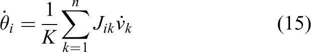
The calculated angular velocity won’t be too large because of the limited parameters, such as K, J_ik and ${\dot{v}}_k$ . The same parameters of the previous DLS simulation are used to evaluate this method.

Obviously, Figure 8(a) and (b) is in deep contrast with Figure 7(a) and (b). We can conclude that the proposed method can guarantee the orientation of the calculated velocity is the same as the original velocity in operation space.

Figure 8.

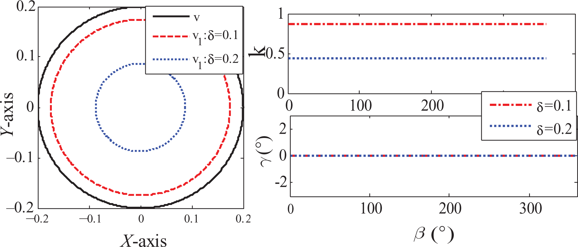
Proposed method (a) Velocity in the operation space and (b) ratio and angle difference of the velocity.

As shown in Figure 9, the proposed method can decrease the angular velocity by selecting δ. From Figures 8 and 9, we can make the conclusion that the proposed method really can avoid too large joint angular velocity and can maintain the direction of the terminal velocity in operational space.

Figure 9.

Angular velocity in joint space by the proposed method.

To design the controller in Figure 4, we need to deduce the dynamic model of the swing leg of the exoskeleton based on coordinate system in Figure 5. Lagrange dynamics is adopted and equation (16) is the dynamic model of the swing leg

$\left[\begin{array}{c}{\tau }_1\\ {\tau }_2\end{array}\right]=\left[\begin{array}{cc}\begin{array}{c}{d}_{11}\\ d_{21}\end{array}& \begin{array}{c}{d}_{12}\\ d_{22}\end{array}\end{array}\right][\begin{array}{c}{\ddot{\theta }}_1\\ {\ddot{\theta }}_2\end{array}]+\left[\begin{array}{cc}\begin{array}{c}{h}_{11}\\ h_{21}\end{array}& \begin{array}{c}{h}_{12}\\ h_{22}\end{array}\end{array}\right]\left[\begin{array}{c}{\dot{\theta }}_1\\ {\dot{\theta }}_2\end{array}\right]+\left[\begin{array}{c}{g}_{11}\\ g_{21}\end{array}\right]$

16

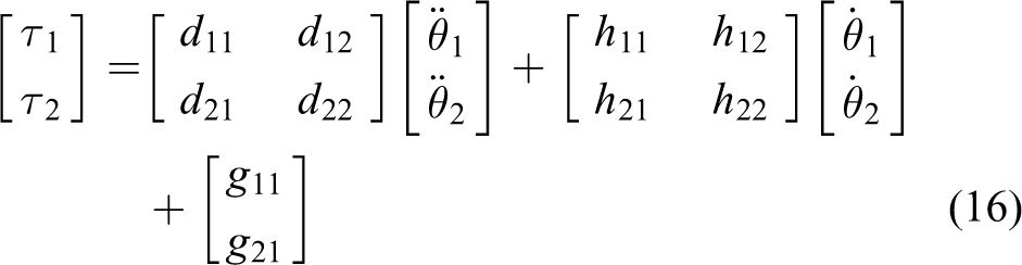
where τ₁ means the hip torque and τ₂ means the knee torque.

Controller design

During designing, the controller based on the model in equation (16), the model error and uncertainties of the actual system are not negligible. The whole dynamics model can be written as

$\left(M+\Delta M\right)\ddot{\theta }+\left(C+\Delta C\right)\dot{\theta }+\left(G+\Delta G\right)=\tau +d$

17

where ΔM, ΔC and ΔG mean the model error, d means the disturbances.

Intuitively, the model error and disturbance are thought of the disturbance and represented by f(t) which is non-linear and difficult to model. f(t) is with boundary as

$f_L\le f(t)\le f_U$

18

Equation (17) can be written as

$M\ddot{\theta }+H\dot{\theta }+G=\tau +f(t)$

19

In traditional sliding mode control,^28,29 the integral sliding surface is designed as follows

$s=ce+\dot{e}+k{\displaystyle {\int }_0^{t}e}dt$

20

where $c=diag[\begin{array}{ccc}{c}_1& \cdots & c_n\end{array}]$ , c_i > 0, $k=diag[\begin{array}{cc}{k}_1\cdots & k_n\end{array}]$ and K_i > 0 are the design parameters which satisfy Hurwitz; e = θ _d − θ means the tracking error.

The third part in equation (20) will lead to the large error accumulation, and may deteriorate the system performance, such as wind-up. Obviously, arctan function atan(x) is a non-linear saturation function and a monotonically increasing function. So another class of quasi-potential function and its derivative is introduced in equation (21)

$Sat(\sigma ·x)=(\sigma x)·\text{atan}\left(\sigma x\right)-\frac{1}{2}\ln \left[1+{(\sigma x)}^2\right];sat(\sigma ·x)=\text{atan}(\sigma x)$

21

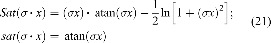
To avoid wind-up, the integral part of equation (20) is replaced by equation (21). The improved sliding surface is written as

$s=ce+\dot{e}+k·Sat(\sigma ·e)$

22

Based on the sliding surface equation (22) and the dynamic model equation (19), we have

$\dot{s}=c\dot{e}+\ddot{e}+k·\text{atan}(\sigma ·e)=c\dot{e}+\left[{\ddot{\theta }}_d-M^{-1}(\tau +f-H\dot{\theta }-G)\right]+k·\text{atan}(\sigma ·e)$

23

To achieve better performance and decrease the reaching time, we have chosen the general sliding model reaching law as

$\dot{s}=-\eta ·{\left|s\right|}^{\alpha }\text{sgn}(s)$

24

where sgn(·) means the sign function, η is a positive switching gain, 0 < α < 1, which can guarantee the system reaches the sliding mode in a greater speed when the system state is far away from the sliding mode, and decrease the chattering problem when the system state reaches the sliding mode.

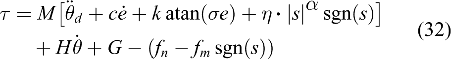
Combining the equations (23) and (24), the control law can be designed as

$\tau =M\left[{\ddot{\theta }}_d+c\dot{e}+k\text{atan}(\sigma e)+\eta ·{\left|s\right|}^{\alpha }\text{sgn}(s)\right]+H\dot{\theta }+G-\widehat{f}$

25

where $\widehat{f}$ represents the estimation value of f.

• Stability proof:

Considering a positive definite Lyapunov function as

$V=\raisebox{1ex}{$1$}\!\left/ \!\raisebox{-1ex}{$2$}\right.s^{T}s$

26

Differentiating equation (26) with respect to time yields

$\dot{V}=s·\dot{s}=s({\ddot{\theta }}_d-M^{-1}[\tau +f-H\dot{\theta }-G]+c\dot{e}+k\text{atan}(\sigma e))$

27

Substituting equation (25) into equation (27), equation (27) can then be written as

$\dot{V}=s\left(-\eta ·{\left|s\right|}^{\alpha }\text{sgn}(s)-M^{-1}\left(f-\widehat{f}\right)\right)=-\eta {\left|s\right|}^{\alpha +1}-s{M}^{-1}(f-\widehat{f})\le -s{M}^{-1}(f-\widehat{f})$

28

Combining the equation (18), we can consider two situations to ensure the system is stable

• when s ≥ 0, we can specify $\widehat{f}=f_L$ , which also means $f-\widehat{f}\ge 0$ . Then the global reaching condition is given by:

$\dot{V}\le -s{M}^{-1}\left(f-\widehat{f}\right)\le 0$

29

• when s < 0, we can specify $\widehat{f}=f_H$ , which also means $f-\widehat{f}\le 0$ . Then the global reaching condition is given by:

$\dot{V}\le -s{M}^{-1}\left(f-\widehat{f}\right)\le 0$

30

To express equations (29) to (30), we define

$f_m=\frac{f_H-f_L}{2};f_n=\frac{f_H+f_L}{2}$

31

Hence, equation (25) can be rewritten as

$\tau =M\left[{\ddot{\theta }}_d+c\dot{e}+k\text{atan}(\sigma e)+\eta ·{\left|s\right|}^{\alpha }\text{sgn}(s)\right]+H\dot{\theta }+G-(f_n-f_m\text{sgn}(s))$

32

Thus, we have designed a control law which satisfies a Lyapunov stability criteria. And the system state will reach the sliding mode surface in finite time.

Considering the signum function in equation (32), its discontinuity characteristic will cause the control input to chatter. To circumvent this situation, the boundary layer technique is employed to alleviate the chattering and smooth the control input. So we have introduced saturation switch function as follows:

$sat2(s)=\{\begin{array}{cc}1& s>\Delta \\ \lambda s& \left|s\right|\le \Delta ,\lambda =1/\Delta \\ -1& s<-\Delta \end{array}$

33

where Δ > 0, and it means the threshold of the boundary layer. Outside the boundary layer, the control has the ideal relay characteristic, it will accelerate the state to reach the sliding mode; however, within the boundary layer, the controller is a feedback controller, it will decrease the chattering during the sliding mode switch.

Simulation and experiment

To verify the effectiveness of the proposed human interface model based on RBF NN and the method to calculate the pseudo-inverse Jacobian matrix and the non-linear novel controller, we perform experiment on the swing leg of the lower extremity exoskeleton as shown in Figure 2. The operator will wear the exoskeleton and move his swing leg which is attached to the swing leg of exoskeleton.

The dynamic model has been obtained as illustrated in section ‘Swing leg modelling’ and the parameters in equation (16) are as follows

$d_{11}=m_s{h}_{sg}^2+m_t{h}_{tg}^2+m_s{l}_1^2+m_s{l}_{sg}^2+m_t{l}_{tg}^2-2m_s{h}_{sg}{l}_1\text{sin}({\theta }_2)+2m_s{l}_1{l}_{sg}\text{cos}({\theta }_2)+I_s+I_t{d}_{12}=m_s{h}_{sg}^2+m_s{l}_{sg}^2-m_s{l}_1{h}_{sg}\text{sin}({\theta }_2)+m_s{l}_1{l}_{sg}\text{cos}({\theta }_2)+I_s{d}_{21}=m_s{h}_{sg}^2+m_s{l}_{sg}^2-m_s{l}_1{h}_{sg}\text{sin}({\theta }_2)+m_s{l}_1{l}_{sg}\text{cos}({\theta }_2)+I_s{d}_{22}=m_s{h}_{sg}^2+m_s{l}_{sg}^2+I_s{h}_{11}=-2{\dot{\theta }}_2{l}_1{m}_s(h_{sg}\text{cos}({\theta }_2)+l_{sg}\text{sin}({\theta }_2));h_{12}=-m_s(2l_1(h_{sg}\text{cos}({\theta }_2)+l_{sg}\text{sin}({\theta }_2)))·{\dot{\theta }}_2/2h_{21}=(m_s{l}_1(h_{sg}\text{cos}({\theta }_2)+l_{sg}\text{sin}({\theta }_2)))·{\dot{\theta }}_1;h_{22}=0g_{11}=-m_{s}g(h_{sg}\text{cos}({\theta }_1+{\theta }_2)+l_{sg}\text{sin}({\theta }_1+{\theta }_2)+l_1\text{sin}({\theta }_1))-m_{t}g(h_{tg}\text{cos}({\theta }_1)+l_{tg}\text{sin}({\theta }_1))g_{21}=-m_{s}g(h_{sg}\text{cos}({\theta }_1+{\theta }_2)+l_{sg}\text{sin}({\theta }_1+{\theta }_2))$

The parameters are given in Figure 6. The swing leg is tracking with the reference trajectory as

$q_d(t)=\left[1.2\text{sin}(\pi t);1.5\text{sin}(\pi t)\right](\mathrm{deg})$

34

where both the initial position of the two joints are zero.

The parameters of the uncertainties in equation (25) are set as

$f(t)=\left[0.2\text{\hspace{0.17em}sin}(5\pi t);0.1\text{\hspace{0.17em}sin}(5\pi t)\right]$

35

We compare the proposed INSM with the conventional sliding mode controller ²⁸ (hereafter called CSM). The parameters of the controller in equation (32) are given as

$c_{1/2}=5;k_{1/2}=5;\sigma =1.5;\eta =3;\alpha =0.3;\Delta =1.5$

The torques from the controller are shown in Figure 10. Obviously, the boundary layer in saturation function eliminates the chattering and the CSM has a large chattering using signum function directly. The large chattering makes the wearer uncomfortable. The INSM has a more smooth torque which is more suitable to be applied in human–machine system.

Figure 10.

(a) Control torque of the hip joint in INSM controller; (b) control torque of the knee joint in INSM controller; (c) control torque of the hip joint in CSM controller; (d) control torque of the knee joint in CSM controller. INSM: non-linear sliding mode controller; CSM: conventional sliding mode controller.

Then, INSM is applied to control the swing leg of the lower extremity exoskeleton. The desired trajectory is produced by RBF NN controller based on the human–robot interaction force. So when the wearer moves his leg, the controller drives the swing leg to shadow the motion. The joint angles are measured by encoders attached to the exoskeleton as shown in Figure 2.

In addition, the human–robot interaction force is measured using the six-axis pressure sensors. This force vector is provided by the wearer’s motions to the exoskeleton, so the magnitude and direction of the force vector reflects information of the wearer’s motion. The controller proposed in this article aims to minimize the force vector and finally decreased the force vector to zero. Thus we can justify the controller’s performance by the amplitude of the interaction force vector. Figure 11 shows the results of the experiment.

Figure 11.

(a) Interaction force along the X axis in INSM and CSM controller; (b) interaction force along the Y axis in INSM and CSM controller; (c) tracking error of the hip joint in INSM and CSM controller; (d) tracking error of the knee joint in INSM and CSM controller. INSM: non-linear sliding mode controller; CSM: conventional sliding mode controller.

To evaluate the performance of the controller, we have adopted two evaluating indicators: the first is the root mean square (RMS) residuals and the second is the maximum absolute value, which are defined as

$e_{\text{RMS}}=\sqrt{\frac{1}{N}{\displaystyle \sum _{i=1}^N{e}^2(i)}};e_{\text{max}}=\underset{0\le i\le N}{\text{max}}\left\{\left|e(i)\right|\right\}$

36

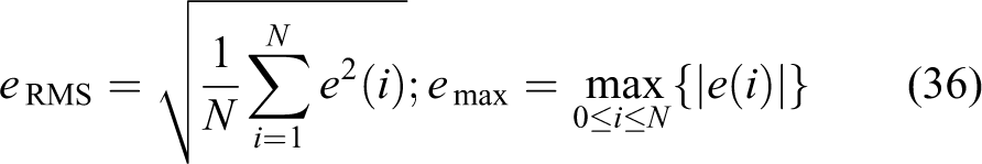
The evaluation results of the controller performance are illustrated in Table 1. Obviously, the RMS value and the maximum value of the two joints gained by INSM controller are much smaller than the corresponding values gained by CSM controller. Because of the accumulation of the error, the CSM controller has a higher maximum absolute tracking error. Compared to other robot system, a more important evaluating indicator is the interaction force. By analysing the interaction force from the force sensor, the RMS value and maximum value are also listed in Table 1. While we adopt the INSM controller, we can get smaller interaction force and the wearer feels more comfortable. The swing leg can shadow the wearer easily. By contrast, the wearer feels bigger interaction force and needs more power to move the swing leg of the lower extremity exoskeleton using the CSM controller.

Table 1.

Performance evaluation.

	e RMS (°) of joint		e max (°) of joint
	Hip	Knee	Hip	Knee	Fx _RMS (N)	Fx _max (N)	Fy _RMS (N)	Fy _max (N)
INSM	0.0033	0.0449	0.0728	0.5602	164.47	30.774	69.739	21.879
CSM	0.0435	0.3199	0.3776	1.3841	905.42	55.428	334.92	55.428

INSM: non-linear sliding mode controller; CSM: conventional sliding mode controller; RMS: root mean square.

Conclusion

In this article, the RBF NN is introduced to model the human–robot interaction which is normally described by impedance model alternatively. The method can depict the non-linear relationship more precisely. Then a new method is proposed to solve the pseudo-inverse Jacobian matrix when the joints reach the kinematic regularity. Analysis and comparative simulation of the swing leg of the exoskeleton has proved that the velocity calculated using the new method can avoid too large amplitude and guarantee the same direction to the real velocity. Further, because of the uncertainties of the human–robot interaction system, an improved robust non-linear integral sliding mode controller has been proposed with a novel non-linear integral sliding surface. It can decrease the reaching time and avoid too large accumulation of the error. Finally, the proposed methods in this article are designed to control the swing leg of the lower extremity exoskeleton to shadow the wearer without given trajectory. Simulation and experiments prove the effectiveness and reliability of the proposed controller compared to traditional sliding mode controller. The wearer also feels more comfortable to move the swing leg using the controller in this article. These proposed methods can be applied in stance leg of the lower extremity exoskeleton and other human–robot interaction system.