DRHC synthesis for simultaneous tracking and formation of nonhomogeneous multi-agents with time-varying communication topology

Abstract

The synthesis approach of distributed receding horizon control is studied for the simultaneous tracking and formation problem of nonhomogeneous multi-agents. Different from the existing works, the communication topology between multi-agents is allowed to be time-varying in this article, which meets miscellaneous conditions in practice. To accommodate the time-varying communication topology, we refresh at each sampling instant the individual cost function for each agent, according to the real-time neighbourhood. Moreover, to guarantee the exponential stability of the overall closed-loop system, we design an auxiliary constraint and impose it in the individual optimization problem. The recursive feasibility of the auxiliary constraint can be guaranteed by updating the formation weighting scalars in real time. By solving the individual optimization problem (with respect to the input, state and auxiliary constraints) at each sampling instant, each agent can obtain its optimal control input sequence. The implementation of the first control input among the sequence for each agent can steer the overall multi-agent system to cooperatively achieve the desired tracking and formation objective. The effectiveness and practicability of our results are demonstrated through the illustrative examples.

Introduction

Due to the advantages in handling the physical constraints and optimizing the control performance, the receding horizon control (RHC), also called model predictive control, has become more and more popular in the control academia. The surveys of RHC can be found in the studies by Garcia et al. ¹ and Mayne et al. ² In RHC, the controller solves a constrained optimization problem (with respect to the cost function and the physical constraints associated with the future evolutions) at each sampling instant to obtain the optimal input sequence but implements only the first element among this sequence. However, the computation burden of RHC handling in the centralized form is usually tremendous, even intolerable, for the systems with high dimensional state variables (see the multi-agent systems and the large-scale industry systems). An efficient paradigm to tackle this issue is partitioning the overall system into a set of subsystems and applying a distributed RHC (DRHC) strategy for each subsystem. ^{3 –6}

For the multi-agent systems, more and more attentions have been attracted on many important fields of research, such as the flocking problem, ^{7 –9} the consensus problem ^{10 –12} and the tracking and/or formation problem, ^{5,6,13 –16} and many approaches have been proposed for the DRHC of these systems. ^{3,5,6,13,17 –19} In this article, we focus on the simultaneous tracking and formation problem of these systems and the DRHC synthesis approach for this problem. In DRHC, the optimization problems of agents can be solved synchronously to save the time for all agents obtaining their control inputs ^5,6 ; however, each agent has to use the assumed future evolutions of its neighbours (usually taken as the predicted evolutions solved at the last instant ^5,6,13,18 ). As a result, the traditional stability paradigm of centralized strategy ^2,20,21 is no longer suitable. To achieve the closed-loop stability guarantee in DRHC, some additional conditions or constraints are usually required for each agent, see for example, the sufficient stability condition derived in the study by Keviczky et al., ¹⁷ the additional contractive constraint employed in the study by Camponogara et al. ³ and the compatibility constraints proposed in the literature. ^13,18 Especially in the study by Wang and Ding, ^5,6 the compatibility constraints are derived and imposed not only to guarantee the closed-loop stability but also to contribute to the collision avoidance.

However, all the above cited works study the DRHC for multi-agent systems based on the fixed communication topology, which fail when any communication link disconnects due to out of distance limitation, data packet dropout and so on. In practice, it is more reasonable to consider the time-varying communication topology due to miscellaneous reasons. Taking the time-varying topology into account, most of the researches focus on the consensus problem. ^{10,12,14,22,23} As reported in the study by Ferrari-Trecate et al., ¹⁰ because of the receding horizon technique, the value of the consensus point depends not only on the initial conditions of the system but also on the sequence of agents’ states and on the communication topology along time. Thus, for the simultaneous tracking and formation problem, in which the objective to be achieved is pre-specified, the DRHC with respect to time-varying communication topology is still an issue to be solved.

Aiming at the simultaneous tracking and formation problem of nonhomogeneous multi-agent systems with time-varying communication topology, we contribute in this article to present a practicable DRHC synthesis approach by (i) online generating the real-time individual cost function for each agent, according to the pre-specified objective, the time-varying communication topology and the real-time updated formation weighing scalar; (ii) deriving an individual condition for each agent, collection of which can guarantee the closed-loop stability of the overall multi-agent system; and (iii) handling the derived condition as an auxiliary constraint and imposing it in the individual optimization problem with recursive feasibility guarantee. Following the imposed auxiliary constraint, the online generated cost function is substituted by its upper bound to be minimized, which endows the auxiliary constraint with the role of enhancing tracking and formation.

The following of this article is organized as follows. The various symbols used in this article are clarified in Table 1. In ‘System description and cost functions’ section, the systems of the multi-agent and reference object, the description of the simultaneous tracking and formation objective, the communication condition and the definition of neighbourhood are introduced. Then the individual cost function of each agent is online generated accordingly. In ‘Stability condition for the multi-agent system with primary distributed RHC’ section, the sufficient closed-loop stability condition of the overall multi-agent system is derived, with respect to the time-varying communication topology. ‘DRHC synthesis’ section then presents the DRHC synthesis approach by distributing the sufficient stability condition into individual ones, handling the individual condition as an auxiliary constraint with recursive feasibility, substituting the original cost function by its upper bound and providing the DRHC implementation algorithm. The properties of the proposed DRHC algorithm is analysed in ‘Property analysis’ section. Additionally, for easy application of the presented DRHC, ‘The optimization problem in LMIs form’ section provides a procedure to transform the individual optimization problem into linear matrix inequalities (LMIs) form, which completes the presentation of the DRHC approach. In ‘Illustrative examples’ section, the numerical and simulation examples are provided to demonstrate the effectiveness and practicability of our results. The ‘Conclusion’ section ends this article.

Table 1.

Notations.

Symbols	Meaning
${\mathcal{N}}_a$	Number of agents ( ${\mathcal{N}}_a\ge 1$ )
ℕ a	Index set of agents, $\{1,2,\dots ,{\mathcal{N}}_a\}$
|ℕ a |	Cardinality of the set ℕ a
ℕ, ℕ−, ℕ+	$\{0,1,\dots ,N-1\},\{0,1,\dots ,N-2\},\{1,2,\dots ,N-1\}$
ℝ n	n-dimensional Euclidean space
${ℝ}^{m\times n}$	m × n-dimensional real matrix set
In	n-order identity matrix
$\text{diag}\{\cdots \}$	A block-diagonal matrix
⋆	Symmetric term with appropriate dimension in a block matrix
P > 0	Positive-definite matrix P
$\overline{\lambda }(P),\underset{¯}{\lambda }(P)$	Maximum, minimum eigenvalues of matrix P
$\parallel x\parallel ,\parallel x{\parallel }_P$	Two-norm of x, P-weight two-norm of x (i.e. $\parallel x\parallel =\sqrt{x^{\text{T}}x},\parallel x{\parallel }_P=\sqrt{x^{\text{T}}Px}$ )
$x(t|k)$	Future value of $x(k+t)$ , predicted at the instant k
$u^{\ast },u^{\circ }$	Values of u corresponding to the optimal, feasible solutions of optimization
$[v;w]$	${[v^T,w^T]}^T$

System description and cost functions

Consider a multi-agent system with ${\mathcal{N}}_a$ agents, which has the following discrete-time dynamic equations

$x_i\left(k+1\right)=A_i{x}_i\left(k\right)+B_i{u}_i\left(k\right),i\in {\mathbb{N}}_a,k\ge 0$

1

where $x_i(k)=[p_i(k);v_i(k)]\in {ℝ}^{2n_i}\text{ and }{u}_i(k)\in {ℝ}^{m_i}$ denote the measurable state vector and control input of agent i, respectively; $p_i(k)\in {ℝ}^{n_i}\text{ and }{v}_i(k)\in {ℝ}^{n_i}$ denote the position and velocity of agent i in n_i-D space, respectively. Usually, the state and input of each agent i are required to satisfy

$x_i\left(k\right)\in {\mathbb{X}}_i=\left\{x_i\in {ℝ}^{2n_i}|\parallel {\Psi }_{i,s}{x}_i\parallel \le {\overline{\psi }}_{i,s},s=1,2,\dots ,c_i^x\right\},k\ge 0$

2

$u_i\left(k\right)\in {\mathbb{U}}_i=\left\{u_i\in {ℝ}^{m_i}|\parallel {\Phi }_{i,s}{u}_i\parallel \le {\overline{\phi }}_{i,s},s=1,2,\dots ,c_i^u\right\},k\ge 0$

3

where the bounded convex set ${\mathbb{X}}_i({\mathbb{U}}_i)$ denotes the admissible state (input) set, ${\Psi }_{i,s}\in {ℝ}^{n_{i,s}^x\times 2n_i}\text{ with }{n}_{i,s}^x\text{ rows and }{\overline{\psi }}_{i,s}>0({\Phi }_{i,s}\in {ℝ}^{m_{i,s}^u\times m_i}\text{ with }{m}_{i,s}^u\text{ rows and }{\overline{\phi }}_{i,s}>0)$ are the state (input) constraint parameters and $c_i^x(c_i^u)$ is the number of the state (input) constraints, of agent i. The reference agent to be tracked has the dynamics

$x_r\left(k+1\right)=A_r{x}_r\left(k\right)+B_r{u}_r\left(k\right),k\ge 0$

4

where $x_r\left(k\right)=\left[p_r\left(k\right);v_r\left(k\right)\right]\in {ℝ}^{2n_r}\text{ and }{u}_r(k)\in {ℝ}^{m_r}$ are the reference state vector and control input, respectively. In this article, the dynamics parameters $\{A_i,B_i\}\text{ and }\{A_r,B_r\}$ are allowed to be different, which accommodates the nonhomogeneous multi-agents.

The control objective of this article is to steer the multi-agents to simultaneously track the reference agent and achieve a pre-specified formation, without violating the required constraints (2) and (3). According to a simultaneous tracking and formation objective desired for the multi-agents, we denote $d_{ir}^p\in {ℝ}^{n_i}$ as the desired tracking position vector between agent i and reference agent, $d_{ij}^p\in {ℝ}^{n_i}$ as the desired formation position vector between the agents i and j, $d_{ir}^x=[d_{ir}^p;0]\in {ℝ}^{2n_i}\text{ and }{d}_{ij}^x=[d_{ij}^p;0]\in {ℝ}^{2n_i}$ as the associated state vectors, $\mathbb{F}=\{(i,j)\in {\mathbb{N}}_a\times {\mathbb{N}}_a|d_{ij}^p\text{is\hspace{0.17em}desired}\}$ as the desired formation pair index set and ${\mathbb{N}}_i^0=\{j\in {\mathbb{N}}_a|(i,j)\in \mathbb{F}\}$ as the desired neighbour index set ( $j\in {\mathbb{N}}_i^0\iff i\in {\mathbb{N}}_j^0$ ). Because the multi-agents and the reference agent are allowed to be nonhomogeneous, even the dimensions of their states (inputs) can be not identical (i.e. $n_i\ne n_j\ne n_r\text{ and/or }{m}_i\ne m_j\ne m_r$ for i ≠ j), we then define the coordinate transformation functions $F_{ir}^x(\cdot ):{ℝ}^{2n_r}\to {ℝ}^{2n_i},F_{ir}^u(\cdot ):{ℝ}^{m_r}\to {ℝ}^{m_i}\text{ and }{F}_{ij}^x(\cdot ):{ℝ}^{2n_j}\to {ℝ}^{2n_i}$ and formulate the control objective in a specific form as

$\text{Tracking}:\underset{k\to \infty }{{\displaystyle \text{lim}}}\left[x_i\left(k\right)-F_{ir}^x\left(x_r\left(k\right)\right)\right]=d_{ir}^x\text{\hspace{0.17em}and\hspace{0.17em}}\underset{k\to \infty }{{\displaystyle \text{lim}}}\left[u_i\left(k\right)-F_{ir}^u\left(u_r\left(k\right)\right)\right]=0,\forall i\in {\mathbb{N}}_a$

5

$\text{Formation}:\underset{k\to \infty }{{\displaystyle \text{lim}}}\left[x_i\left(k\right)-F_{ij}^x\left(x_j\left(k\right)\right)\right]=d_{ij}^x,\forall j\in {\mathbb{N}}_i^0$

6

To guarantee the desired control objective being realizable for the multi-agents, the following assumption is required.

Assumption 1

The multi-agents and reference agent are compatible, and the simultaneous tracking and formation objective is achievable, that is, the coordinate transformation functions and the desired vectors satisfy

$\text{Compatibility: }{F}_{ir}^x(x_r\left(k+1\right))+d_{ir}^x=A_i\left(F_{ir}^x\left(x_r\left(k\right)\right)+d_{ir}^x\right)+B_i{F}_{ir}^u\left(u_r\left(k\right)\right),\forall i\in {\mathbb{N}}_a,k\ge 0$

7

$\text{Trackability: }{F}_{ir}^x\left(x_r\left(k\right)\right)+d_{ir}^x\in {\mathbb{X}}_i\text{\hspace{0.17em}and\hspace{0.17em}}{F}_{ir}^u\left(u_r\left(k\right)\right)\in {\mathbb{U}}_i,\forall i\in {\mathbb{N}}_a,k\ge 0$

8

$\text{Consistency: }{d}_{ij}^x=d_{ir}^x-F_{ij}^x\left(d_{jr}^x\right)=d_{il}^x-F_{ij}^x\left(d_{jl}^x\right),\forall \left(i,j\right),\left(i,l\right),\left(j,l\right)\in \mathbb{F}$

9

Additionally, the function $F_{ij}^x(\cdot )$ is Lipschitz, that is, there exists a constant ${\overline{F}}_{ij}^x>0\text{ such that }\parallel F_{ij}^x(x)\parallel \le {\overline{F}}_{ij}^x\parallel x\parallel ,\forall x\in {ℝ}^{n_j},(i,j)\in \mathbb{F}$ .

Due to miscellaneous practical conditions, such as the distance limitation of effective communication, communication delays, data packet dropouts and so on, the communication topology is usually time-varying. Thus, the neighbourhood between agents needs a real-time presentation, which is defined as follows.

Definition 1

At each instant k, the agent j is a real-time neighbour of agent i if it is a desired neighbour of agent i and agent i can receive data from agent j. Hence, the real-time neighbour index set of agent i can be formulated as ${\mathbb{N}}_i(k)=\{j\in {\mathbb{N}}_i^0|\text{agent\hspace{0.17em}}i\text{\hspace{0.17em}can\hspace{0.17em}receive\hspace{0.17em}data\hspace{0.17em}from\hspace{0.17em}agent\hspace{0.17em}}j\text{\hspace{0.17em}at\hspace{0.17em}the\hspace{0.17em}}k\text{th\hspace{0.17em}instant}\}$ .

Note that $j\in {\mathbb{N}}_i(k)\nLeftrightarrow i\in {\mathbb{N}}_j(k)$ due to different conditions. According to the above control objective and time-varying neighbourhood, we generate the ideal real-time individual cost function for each agent i as

$J_i\left(x_{ir},x_{i\blacksquare },u_{ir},k\right)=\underset{\text{tracking\hspace{0.17em}cost}}{\underbrace{{\displaystyle \sum _{t\in \mathbb{N}}}\left({\alpha }_i\parallel x_{ir}\left(t|k\right){\parallel }^2+{\rho }_i\parallel u_{ir}\left(t|k\right){\parallel }^2\right)}}+\underset{\text{formation\hspace{0.17em}cost}}{\underbrace{{\displaystyle \sum _{t\in \mathbb{N}}}{\displaystyle \sum _{j\in {\mathbb{N}}_i(k)}}{\beta }_i\parallel x_{ij}\left(t|k\right){\parallel }^2}}+\underset{\text{terminal\hspace{0.17em}cost}}{\underbrace{\parallel x_{ir}\left(N|k\right){\parallel }_{P_i(k)}^2}}$

10

where N is the predictive horizon; $x_{ir}(t|k)=x_i(t|k)-F_{ir}^x(x_r(k+t))-d_{ir}^x,x_{ij}(t|k)=x_i(t|k)-F_{ij}^x(x_j(t|k))-d_{ij}^x=x_{ir}(t|k)-F_{ij}^x(x_{jr}(t|k))\text{ and }{u}_{ir}(t|k)=u_i(t|k)-F_{ir}^u(u_r(k+t))$ denote the predictive deviations; ${\alpha }_i>0\text{ and }{\rho }_i>0$ are the pre-specified tracking weighting scalars; ${\beta }_i>0$ is the pre-specified formation weighting scalar; $P_i(k)>0$ is the terminal weighting matrix determined in real time.

For brief expression, the cost function (10) can be reformulated as

$J_i\left(x_{ir},x_{i\blacksquare },u_{ir},k\right)={\displaystyle \sum _{t\in \mathbb{N}}}\left(\parallel z_{ir}\left(t|k\right){\parallel }_{Q_i(k)}^2+\parallel u_{ir}\left(t|k\right){\parallel }_{R_i}^2\right)+\parallel x_{ir}\left(N|k\right){\parallel }_{P_i(k)}^2$

11

where $z_{ir}=[x_{j_1,r};\cdots ;x_{j_{|{\mathbb{N}}_i^0|},r};x_{ir}]\in {ℝ}^{2n_i}$ is the local collected vector, with $\{j_1,\cdots ,j_{|{\mathbb{N}}_i^0|}\}={\mathbb{N}}_i^0\text{ and }{\mathit{n}}_i={\displaystyle {\sum }_{j\in {\mathbb{N}}_i^0}}{n}_j+n_i;Q_i(k)>0\text{ and }{R}_i>0$ are the local weighting matrices calculated according to α_i, ρ_i and β_i as in proposition 1.

Proposition 1

$R_i={\rho }_i{I}_{m_i}\text{ and }{Q}_i(k)=G_i^T{W}_i(k)G_i$ with

$G_i=\left[\begin{array}{ccccc}-F_{i,j_1}^x(\cdot )& 0& \cdots & 0& I_{2n_i}\\ 0& -F_{i,j_2}^x(\cdot )& \ddots & ⋮& I_{2n_i}\\ ⋮& \ddots & \ddots & 0& ⋮\\ 0& \cdots & 0& -F_{i,j_{|{\mathbb{N}}_i^0|}}^x(\cdot )& I_{2n_i}\\ 0& \cdots & \cdots & 0& I_{2n_i}\end{array}\right]\in {ℝ}^{2(|{\mathbb{N}}_i^0|+1)n_i\times 2{\mathit{n}}_i},\{j_1,j_2,\cdots ,j_{|{\mathbb{N}}_i^0|}\}={\mathbb{N}}_i^0$

12

and $W_i(k)=\text{diag}\{w_{i\mathrm{,1}}(k)I_{2n_i},\cdots ,w_{i,|{\mathbb{N}}_i^0|}(k)I_{2n_i},{\alpha }_i{I}_{2n_i}\},\text{ where }{w}_{i,s}(k)=\{\begin{array}{cc}{\beta }_i,& \text{\hspace{0.05em}the\hspace{0.17em}}s\text{th\hspace{0.17em}element\hspace{0.17em}of\hspace{0.17em}}{\mathbb{N}}_i^0\text{\hspace{0.17em}belongs\hspace{0.17em}to\hspace{0.17em}}{\mathbb{N}}_i(k);\\ 0,& \text{\hspace{0.05em}otherwise\hspace{0.05em}}\end{array}\text{ for }s\in \{1,2,\dots ,|{\mathbb{N}}_i^0|\}$

According to equation (11), the brief expression of the global cost function can be formulated for the multi-agent system as

$J_{\Sigma }\left(k\right)={\displaystyle \sum _{i\in {\mathbb{N}}_a}}{J}_i\left(x_{ir},x_{i\blacksquare },u_{ir},k\right)={\displaystyle \sum _{t\in \mathbb{N}}}\left(\parallel z_{\Sigma r}\left(t|k\right){\parallel }_{Q(k)}^2+\parallel u_{\Sigma r}\left(t|k\right){\parallel }_R^2\right)+\parallel z_{\Sigma r}\left(N|k\right){\parallel }_{P(k)}^2$

13

where $z_{\Sigma r}=[x_{1r};x_{2r};\cdots ;x_{{\mathcal{N}}_a,r}]\in {ℝ}^{2\mathit{n}}\text{ and }{u}_{\Sigma r}=[u_{1r};u_{2r};\cdots ;u_{{\mathcal{N}}_a,r}]\in {ℝ}^{\mathit{m}}$ are the global collected vectors, with $\mathit{n}={\displaystyle {\sum }_{i\in {\mathbb{N}}_a}}{n}_i\text{ and }\mathit{m}={\displaystyle {\sum }_{i\in {\mathbb{N}}_a}}{m}_i;Q(k)>0,R>0\text{ and }P(k)>0$ are the associated global weighting matrices determined as in proposition 2.

Proposition 2

$P(k)=\text{diag}\{P_1(k),\cdots ,P_{{\mathcal{N}}_a}(k)\},R=\text{diag}\{R_1,\cdots ,R_{{\mathcal{N}}_a}\}\text{ and }Q(k)={\mathcal{G}}^{\text{T}}W(k)\mathcal{G},\text{ where }W(k)=\text{diag}\{W_1(k),\cdots ,W_{{\mathcal{N}}_a}(k)\}\text{ with }{W}_i(k)$ formulated in proposition 1, and $\mathcal{G}=[{\mathcal{G}}_1;\cdots ;{\mathcal{G}}_{{\mathcal{N}}_a}]$ with

${\mathcal{G}}_i=\left[\begin{array}{ccc}{\mathcal{G}}_i^{1,1}& \cdots & {\mathcal{G}}_i^{1,{\mathcal{N}}_a}\\ ⋮& \ddots & ⋮\\ {\mathcal{G}}_i^{|{\mathbb{N}}_i^0|+1,1}& ⋮& {\mathcal{G}}_i^{|{\mathbb{N}}_i^0|+1,{\mathcal{N}}_a}\end{array}\right]\in {ℝ}^{2(|{\mathbb{N}}_i^0|+1)n_i\times 2\mathit{n}},{\mathcal{G}}_i^{pq}=\{\begin{array}{ll}{I}_{2n_i},\hfill & q=i,p=1,\dots ,|{\mathbb{N}}_i^0|,|{\mathbb{N}}_i^0|+1;\hfill \\ -F_{i,q}^x(\cdot ),\hfill & q\text{\hspace{0.17em}is\hspace{0.17em}the\hspace{0.17em}}p\text{th\hspace{0.17em}element\hspace{0.17em}of\hspace{0.17em}}{\mathbb{N}}_i^0;\hfill \\ 0,\hfill & \text{\hspace{0.05em}otherwise\hspace{0.05em}}\hfill \end{array}$

14

Due to the time-varying matrix $W_i(k)$ has a natural upper bound ${\overline{W}}_i=\text{diag}\{{\beta }_i{I}_{2n_i},\cdots ,{\beta }_i{I}_{2n_i},{\alpha }_i{I}_{2n_i}\}\text{ for any }i\in {\mathbb{N}}_a$ , the upper bounds of the real-time local weighting matrix $Q_i(k)$ and global weighting matrix Q(k) can be easily determined as ${\overline{Q}}_i=G_i^T{\overline{W}}_i{G}_i\text{ and }\overline{Q}={\mathcal{G}}^T\text{diag}\{{\overline{W}}_1,\cdots ,{\overline{W}}_{{\mathcal{N}}_a}\}\mathcal{G}$ , respectively.

Stability condition for the multi-agent system with primary distributed RHC

According to the traditional RHC synthesis approach in the study by Mayne et al., ² imposing $x_i(N|k)\in {\mathbb{X}}_i^f(N|k)\text{ with }{\mathbb{X}}_i^f(N|k)$ being a terminal constraint set is a common practice for stability. ^5,18 Generally, the terminal constraint set ${\mathbb{X}}_i^f(N|k)$ is chosen to be admissible and positively invariant. Here, we intend to describe the admissible and positively invariant set for each agent i, by the following terminal constraints

$\parallel x_{ir}\left(N|k\right){\parallel }_{P_i(k)}^2\le {\epsilon }_i\left(k\right)$

15

$\parallel x_{ir}^K\left(t+1|k\right){\parallel }_{P_i(k)}^2-\parallel x_{ir}^K\left(t|k\right){\parallel }_{P_i(k)}^2\le -\parallel x_{ir}^K\left(t|k\right){\parallel }_{\overline{\lambda }(\overline{Q})I_{2n_i}}^2-\parallel u_{ir}^K\left(t|k\right){\parallel }_{R_i}^2,\forall t\ge N$

16

$x_i^K\left(t|k\right)\in {\mathbb{X}}_i,\forall t\ge N$

17

$u_i^K\left(t|k\right)=K_i\left(k\right)x_{ir}^K\left(t|k\right)+F_{ir}^u(u_r\left(k+t\right))\in {\mathbb{U}}_i,\forall t\ge N$

18

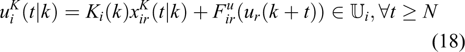
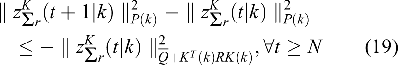
where ${\epsilon }_i(k)$ is a positive scalar; $x_{ir}^K\text{ and }{u}_{ir}^K$ are the deviations corresponding to $x_i^K\text{ and }{u}_i^K$ , respectively; $x_i^K(t+1|k)$ is obtained along the dynamics (1) by implementing $u_i^K(t|k)=K_i(k)x_{ir}^K(t|k)+F_{ir}^u(u_r(k+t)),\text{ with }{x}_{ir}^K(N|k)=x_{ir}^{\ast }(N|k);K_i(k)$ is the terminal state feedback law. Hence, ${\mathbb{X}}_i^f(N|k)=\{x_i(N|k)|(15)-(18)\}$ is defined. For $x_i(N|k)\in {\mathbb{X}}_i^f(N|k)$ , by summing (16) for all $i\in {\mathbb{N}}_a$ , with respect to equation (18), we have

$\parallel z_{\Sigma r}^K(t+1|k){\parallel }_{P(k)}^2-\parallel z_{\Sigma r}^K(t|k){\parallel }_{P(k)}^2\le -\parallel z_{\Sigma r}^K(t|k){\parallel }_{\overline{Q}+K^T(k)RK(k)}^2,\forall t\ge N$

19

where $z_{\Sigma r}^K=[x_{1r}^K;x_{2r}^K;\cdots ;x_{{\mathcal{N}}_a,r}^K]\text{ and }K(k)=\text{diag}\{K_1(k),\cdots ,K_{{\mathcal{N}}_a}(k)\}$ .

Remark 1

In this article, the parameters ${\epsilon }_i(k),P_i(k)\text{ and }{K}_i(k)$ are solved online. Alternatively, one can fix ε_i, P_i and K_i offline ⁵ for less online computational burden. Compared with the offline choice, online solution with relaxed terminal constraints can improve the control performance and enlarge the attraction region, ^18,24 which prefers to be adopted in this article.

To implement an RHC strategy in the distributed way, each agent i has to utilize the future evolution $x_j(t|k),j\in {\mathbb{N}}_i(k)$ to minimize the ideal cost function (10). Because the future evolution is not determined before optimization, an assumed evolution ${\widehat{x}}_j(t|k)$ has to be adopted as substitution. Generally, the assumed evolution is chosen as the optimal one solved at the last instant, ^5,6,13,18 that is, each agent $i\in {\mathbb{N}}_a\text{ broadcasts }{\widehat{x}}_i(t|k)=x_i^{\ast }(t+1|k-1),t\in \mathbb{N}$ as its future evolution before the current optimization. This manner brings to the actual cost function $J_i(x_{ir},{\widehat{x}}_{i\blacksquare },u_{ir},k)$ , which is constructed by substituting $x_{ij}(t|k)$ in equation (10) with ${\widehat{x}}_{ij}(t|k)=x_i(t|k)-F_{ij}^x({\widehat{x}}_j(t|k))+d_{ij}^x$ .

Following the above procedures, each agent $i\in {\mathbb{N}}_a$ can apply a primary DRHC strategy by solving the individual receding horizon optimization problem

$\underset{{\epsilon }_i(k),P_i(k),K_i(k),u_i(t|k),t\in \mathbb{N}}{{\displaystyle \text{min}}}{J}_i\left(x_{ir},{\widehat{x}}_{i\blacksquare },u_{ir},k\right)$

20

$\text{subject\hspace{0.17em}to\hspace{1em}\hspace{1em}\hspace{1em}}{x}_i\left(0|k\right)=x_i\left(k\right)$

21

$x_i\left(t+1|k\right)=A_i{x}_i\left(t|k\right)+B_i{u}_i\left(t|k\right),t\in \mathbb{N}$

22

$x_i\left(t+1|k\right)\in {\mathbb{X}}_i,t\in {\mathbb{N}}^{+}$

23

$u_i\left(t|k\right)\in {\mathbb{U}}_i,t\in \mathbb{N}$

24

$x_i\left(N|k\right)\in {\mathbb{X}}_i^f\left(N|k\right)=\left\{x_i\left(N|k\right)|(15)-(18)\right\}$

25

and implementing the first element of the optimal control input, that is, $u_i(k)=u_i^{\ast }(0|k)$ . From the property of traditional RHC synthesis approach, the recursive feasibility of the distributed optimization problem (20 to 25) can be naturally guaranteed, by choosing the current feasible solution as

${\epsilon }_i^{\circ }\left(k+1\right)={\epsilon }_i^{\ast }\left(k\right),P_i^{\circ }\left(k+1\right)=P_i^{\ast }\left(k\right),K_i^{\circ }\left(k+1\right)=K_i^{\ast }\left(k\right)$

26

$u_i^{\circ }\left(t|k+1\right)=u_i^{\ast }\left(t+1|k\right)\text{for\hspace{0.17em}}t\in {\mathbb{N}}^{-},u_i^{\circ }\left(N-1|k+1\right)=u_i^K\left(N|k\right)$

27

However, due to $x_j(t|k)$ is substituted by ${\widehat{x}}_j(t|k)$ , and the time-varying neighbourhood is considered in the actual cost function, the guarantee for the stability of overall multi-agent system requires an additional condition. The required condition can be derived as follows.

According to the common practice of RHC synthesis, we can choose the Lyapunov function as the optimal cost function of the overall multi-agent system, that is, $V(k)={\displaystyle {\sum }_{i\in {\mathbb{N}}_a}}{J}_i(x_{ir}^{\ast },{\widehat{x}}_{i\blacksquare }^{\ast },u_{ir}^{\ast },k)$ . Then, by applying the feasible solution (26 and 27) and utilizing the equation (19), we have

$\begin{array}{l}V\left(k+1\right)-V\left(k\right)\le {\displaystyle \sum _{i\in {\mathbb{N}}_a}}{J}_i\left(x_{ir}^{\circ }\mathrm{,}{\widehat{x}}_{i\blacksquare }^{\circ }\mathrm{,}{u}_{ir}^{\circ }\mathrm{,}k+1\right)-{\displaystyle \sum _{i\in {\mathbb{N}}_a}}{J}_i\left(x_{ir}^{\ast }\mathrm{,}{\widehat{x}}_{i\blacksquare }^{\ast }\mathrm{,}{u}_{ir}^{\ast }\mathrm{,}k\right)\\ ={\displaystyle \sum _{i\in {\mathbb{N}}_a}}{\displaystyle \sum _{t\in \mathbb{N}}}\left({\alpha }_i\parallel x_{ir}^{\circ }\left(t|k+1\right){\parallel }^2+{\rho }_i\parallel u_{ir}^{\circ }\left(t|k+1\right){\parallel }^2+{\displaystyle \sum _{j\in {\mathbb{N}}_i(k+1)}}{\beta }_i\parallel {\widehat{x}}_{ij}^{\circ }\left(t|k+1\right)\parallel \right)+\parallel z_{\Sigma r}^{\circ }\left(N|k+1\right){\parallel }_{P^{\circ }(k+1)}^2\\ -{\displaystyle \sum _{i\in {\mathbb{N}}_a}}{\displaystyle \sum _{t\in \mathbb{N}}}\left({\alpha }_i\parallel x_{ir}^{\ast }\left(t|k\right){\parallel }^2+{\rho }_i\parallel u_{ir}^{\ast }\left(t|k\right){\parallel }^2+{\displaystyle \sum _{j\in {\mathbb{N}}_i(k)}}{\beta }_i\parallel {\widehat{x}}_{ij}^{\ast }\left(t|k\right)\parallel \right)-\parallel z_{\Sigma r}^{\ast }\left(N|k\right){\parallel }_{P^{\ast }(k)}^2\\ \le {\displaystyle \sum _{i\in {\mathbb{N}}_a}}{\displaystyle \sum _{t\in \mathbb{N}}}\left({\displaystyle \sum _{j\in {\mathbb{N}}_i(k+1)}}{\beta }_i\parallel x_{ij}^{\ast }\left(t|k\right){\parallel }^2-{\displaystyle \sum _{j\in {\mathbb{N}}_i(k)}}{\beta }_i\parallel {\widehat{x}}_{ij}^{\ast }\left(t|k\right){\parallel }^2\right)-{\displaystyle \sum _{i\in {\mathbb{N}}_a}}(\parallel z_{ir}\left(k\right){\parallel }_{Q_i(k)}^2+\parallel u_{ir}^{\ast }\left(0|k\right){\parallel }_{R_i}^2)\end{array}$

28

By introducing a pre-specified convergence speed $\delta \in [0,1)$ , we intend to guarantee the exponential stability of the overall multi-agent system, by imposing $V(k+1)-V(k)\le -(1-\delta )\underset{\_}{\lambda }(Q(k))\parallel z_{\Sigma r}(k){\parallel }^2\le 0\text{ for all }k\ge 0$ . Following equation (28), it can be strictly guaranteed by

${\displaystyle \sum _{i\in {\mathbb{N}}_a}}\left[{\displaystyle \sum _{t\in \mathbb{N}}}\left({\displaystyle \sum _{j\in {\mathbb{N}}_i(k+1)}}{\beta }_i\parallel x_{ij}^{\ast }\left(t|k\right){\parallel }^2-{\displaystyle \sum _{j\in {\mathbb{N}}_i(k)}}{\beta }_i\parallel {\widehat{x}}_{ij}^{\ast }\left(t|k\right){\parallel }^2\right)-\delta \parallel z_{ir}\left(k\right){\parallel }_{Q_i(k)}^2\right]\le 0$

29

Because the neighbour index set ${\mathbb{N}}_i(\cdot )$ is time-varying according to the real-time communication topology, one has to consider the extreme case ${\mathbb{N}}_i(k)=Ø$ . Hence, the satisfaction of the inequality (29) further requires

${\displaystyle \sum _{i\in {\mathbb{N}}_a}}\left({\displaystyle \sum _{t\in \mathbb{N}}}{\displaystyle \sum _{j\in {\mathbb{N}}_i(k+1)}}{\beta }_i\parallel x_{ij}^{\ast }\left(t|k\right){\parallel }^2-\delta \parallel z_{ir}\left(k\right){\parallel }_{Q_i(k)}^2\right)\le 0,k\ge 0$

30

which serves as a sufficient exponential stability condition for the overall multi-agent system.

Remark 2

For the multi-agent system with fixed communication topology, that is, ${\mathbb{N}}_i(k)={\mathbb{N}}_i(k+1)={\mathbb{N}}_i^0$ for all k ≥ 0, the inequality (29) also serve as a sufficient exponential stability condition (similar to the condition (38) in the study by Wang and Ding ⁵ ). Then by properly distributing, an individual constraint (see the compatibility constraints in the literature ^5,6,18 ) can be designed and imposed in the individual optimization problem to guarantee stability. However, the time-varying communication topology leads to the sufficient exponential stability condition (30) in this article, which invalidates the design of compatibility constraint. Note that the condition (30) is inevitably more conservative than (29), because the extreme case ${\mathbb{N}}_i(k)=Ø$ must be taken into account.

DRHC synthesis

Based on the sufficient exponential stability condition (30), we synthesize the DRHC in this section as follows.

Distribution of the sufficient stability condition

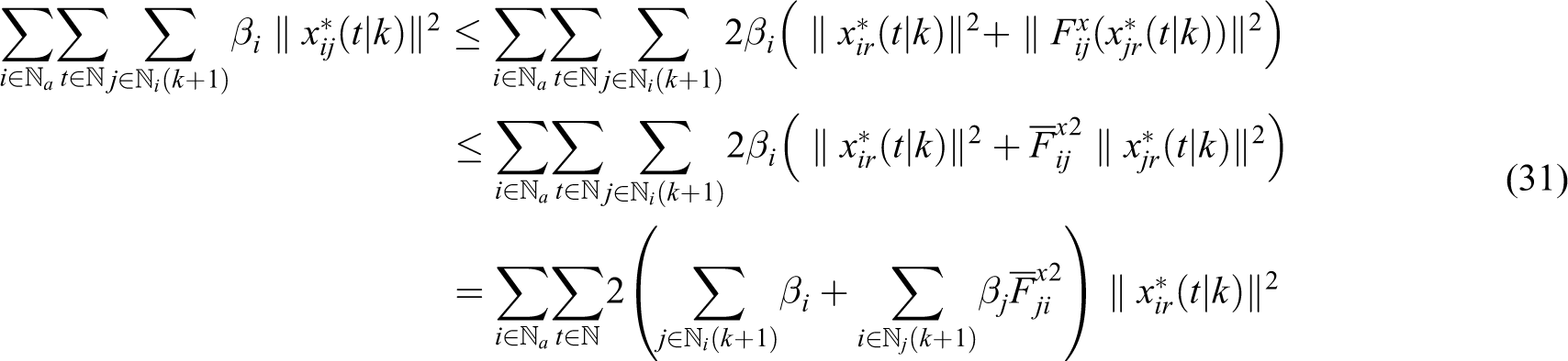
By applying the definition $x_{ij}=x_{ir}-F_{ij}^x(x_{jr})$ and the triangle inequality, we have

$\begin{array}{l}{\displaystyle \sum _{i\in {\mathbb{N}}_a}}{\displaystyle \sum _{t\in \mathbb{N}}}{\displaystyle \sum _{j\in {\mathbb{N}}_i(k+1)}}{\beta }_i\parallel x_{ij}^{\ast }\left(t|k\right){\parallel }^2\le {\displaystyle \sum _{i\in {\mathbb{N}}_a}}{\displaystyle \sum _{t\in \mathbb{N}}}{\displaystyle \sum _{j\in {\mathbb{N}}_i(k+1)}}2{\beta }_i\left(\parallel x_{ir}^{\ast }\left(t|k\right){\parallel }^2+\parallel F_{ij}^x(x_{jr}^{\ast }\left(t|k\right)){\parallel }^2\right)\\ \le {\displaystyle \sum _{i\in {\mathbb{N}}_a}}{\displaystyle \sum _{t\in \mathbb{N}}}{\displaystyle \sum _{j\in {\mathbb{N}}_i(k+1)}}2{\beta }_i\left(\parallel x_{ir}^{\ast }\left(t|k\right){\parallel }^2+{\overline{F}}_{ij}^{x2}\parallel x_{jr}^{\ast }\left(t|k\right){\parallel }^2\right)\\ ={\displaystyle \sum _{i\in {\mathbb{N}}_a}}{\displaystyle \sum _{t\in \mathbb{N}}}2({\displaystyle \sum _{j\in {\mathbb{N}}_i(k+1)}}{\beta }_i+{\displaystyle \sum _{i\in {\mathbb{N}}_j(k+1)}}{\beta }_j{\overline{F}}_{\mathit{\text{ji}}}^{x2})\parallel x_{ir}^{\ast }\left(t|k\right){\parallel }^2\end{array}$

31

which can be substituted into equation (30) to obtain the following distributed condition

${\displaystyle \sum _{t\in \mathbb{N}}}2\left({\displaystyle \sum _{j\in {\mathbb{N}}_i(k+1)}}{\beta }_i+{\displaystyle \sum _{i\in {\mathbb{N}}_j(k+1)}}{\beta }_j{\overline{F}}_{ij}^{x2}\right)\parallel x_{ir}^{\ast }\left(t|k\right){\parallel }^2-\delta \parallel z_{ir}\left(k\right){\parallel }_{Q_i(k)}^2\le 0,\forall i\in {\mathbb{N}}_a$

32

Note in condition (32) that, only the term $\parallel x_{ir}(t|k){\parallel }^2$ is to be solved. Hence, we can assign the condition (32) to each agent as an individual constraint, that is

${\displaystyle \sum _{t\in \mathbb{N}}}\parallel x_{ir}^{\ast }\left(t|k\right){\parallel }^2\le \frac{\delta \parallel z_{ir}\left(k\right){\parallel }_{Q_i(k)}^2}{2\left({\displaystyle \sum _{j\in {\mathbb{N}}_i(k+1)}}{\beta }_i+{\displaystyle \sum _{i\in {\mathbb{N}}_j(k+1)}}{\beta }_j{\overline{F}}_{ij}^{x2}\right)}$

33

Design of an auxiliary constraint

Now, the exponential stability of the overall multi-agent system can be easily guaranteed, by imposing the individual constraint (33) in the optimization problem (20 to 25). However, the constraint (33) cannot be realized due to the undetermined sets ${\mathbb{N}}_i(k+1)$ s, and its satisfaction can be prevented due to the fixed weighting scalars β_i s. Considering this issue, we enforce each agent i to update its formation weighting scalar according to

${\beta }_i\left(k+1\right)=\underset{j\in {\mathbb{N}}_i(k+1)}{{\displaystyle \text{min}}}\left\{{\eta }_i\left(k\right),{\eta }_j\left(k\right),{\overline{\beta }}_i\right\}$

34

where ${\eta }_i(k)$ s are introduced positive decision variables, and ${\overline{\beta }}_i$ is specified as the originally fixed scalar β_i. According to the update equation (34), the following property holds

${\displaystyle \sum _{j\in {\mathbb{N}}_i(k+1)}}{\beta }_i\left(k+1\right)+{\displaystyle \sum _{i\in {\mathbb{N}}_j(k+1)}}{\beta }_j\left(k+1\right){\overline{F}}_{ji}^{x2}\le {\displaystyle \sum _{j\in {\mathbb{N}}_i(k+1)}}{\eta }_i\left(k\right)+{\displaystyle \sum _{i\in {\mathbb{N}}_j(k+1)}}{\eta }_i\left(k\right){\overline{F}}_{ji}^{x2}\le {\eta }_i\left(k\right){\displaystyle \sum _{j\in {\mathbb{N}}_i^0}}\left(1+{\overline{F}}_{ji}^{x2}\right)$

35

Then, the individual constraint (33) is strictly guaranteed by an auxiliary constraint

${\displaystyle \sum _{t\in \mathbb{N}}}\parallel x_{ir}\left(t|k\right){\parallel }^2\le \frac{\delta \parallel z_{ir}\left(k\right){\parallel }_{Q_i(k)}^2}{2{\eta }_i\left(k\right){\Delta }_i}$

36

where ${\Delta }_i={\displaystyle {\sum }_{j\in {\mathbb{N}}_i^0}}(1+{\overline{F}}_{ji}^{x2})$ . It deserves to note that, the constraint (36) can be easily realized by calculating the terms $\parallel z_{ir}(k){\parallel }_{Q_i(k)}^2$ and Δ_i before optimization and can be easily satisfied by choosing a decision variable ${\eta }_i(k)>0$ small enough.

Handling of the cost function

By imposing the auxiliary constraint (36) in the individual optimization problem (20 to 25), both the recursive feasibility and exponential stability can be guaranteed. However, because the auxiliary constraint (36) is more easily satisfiable for a smaller ${\eta }_i(k)$ , directly minimizing the cost function $J_i(x_{ir},{\widehat{x}}_{i\blacksquare },u_{ir},k)$ tends to obtain a smaller ${\eta }_i(k)$ . Then, following the update equation (34), a smaller ${\beta }_i(k+1)$ will be obtained to weaken the formation effort. Hence, we prefer to solve a larger variable ${\eta }_i(k)$ in the optimization. Additionally, the terminal constraint set ${\mathbb{X}}_i^f(N|k)$ prefers a smaller variable ${\epsilon }_i(k)$ . To these ends, we apply the auxiliary constraint (36) and the terminal constraint (15) to determine an upper bound for $J_i(x_{ir},{\widehat{x}}_{i\blacksquare },u_{ir},k)$ as

${\overline{J}}_i\left({\epsilon }_i,{\eta }_i,x_{ir},{\widehat{x}}_{i\blacksquare },u_{ir},k\right)=\left(1+\frac{{\alpha }_i\delta }{2{\eta }_i\left(k\right){\Delta }_i}\right)\parallel z_{ir}\left(k\right){\parallel }_{Q_i(k)}^2+{\displaystyle \sum _{t\in \mathbb{N}}}\left({\rho }_i\parallel u_{ir}\left(t|k\right){\parallel }^2+{\displaystyle \sum _{j\in {\mathbb{N}}_i(k)}}{\beta }_i\left(k\right)\parallel {\widehat{x}}_{ij}\left(t|k\right){\parallel }^2\right)+{\epsilon }_i\left(k\right)$

37

Note in equation (37) that, the upper bound ${\overline{J}}_i({\epsilon }_i,{\eta }_i,x_{ir},{\widehat{x}}_{i\blacksquare },u_{ir},k)$ is inversely proportional to the variable ${\eta }_i(k)$ and proportional to the variable ${\epsilon }_i(k)$ . Hence, the maximum ${\eta }_i(k)$ and the minimum ${\epsilon }_i(k)$ can be solved by minimizing equation (37).

Implementation of DRHC strategy

Following the above procedures, the actual individual optimization problem can be constructed for each agent $i\in {\mathbb{N}}_a$ as

$\underset{{\epsilon }_i\left(k\right),P_i(k),K_i(k),{\eta }_i(k),u_i(t|k),t\in \mathbb{N}}{{\displaystyle \text{min}}}(37)\text{\hspace{1em}subject to\hspace{1em}}(21)-(25)\text{\hspace{0.17em}and\hspace{0.17em}(36)}$

38

based on which the associated DRHC algorithm is presented for implementation as follows.

Algorithm 1

Offline stage: For each agent $i\in {\mathbb{N}}_a$ , determine the set ${\mathbb{N}}_i^0$ according to the given tracking and formation vectors $d_{ir}^p\text{ and }{d}_{ij}^p$ ; determine the functions $F_{ir}^x(\cdot ),F_{ir}^u(\cdot )\text{ and }{F}_{ij}^x(\cdot )$ s according to the dynamics of all agents and calculate the Lipschitz constants ${\overline{F}}_{ij}^x$ s; give the weighting scalars α_i, ρ_i and ${\beta }_i={\overline{\beta }}_i$ and choose the convergence speed $\delta \in [0,1)$ and predictive horizon N ; calculate the scalars $\overline{\lambda }(\overline{Q})\text{ and }{\Delta }_i={\displaystyle {\sum }_{j\in {\mathbb{N}}_i^0}}(1+{\overline{F}}_{ij}^{x2})$ .

Online stage: At the initial instant k = 0, set ${\eta }_i^{\ast }(-1)={\overline{\beta }}_i\text{ and }{\widehat{x}}_i(t|0)=x_i(0)\text{ for all }i\in {\mathbb{N}}_a\text{ and }t\in \mathbb{N}$ . At each instant k ≥ 0, each agent i performs as follows:

Broadcast ${\eta }_i^{\ast }(k-1)\text{ and }{\widehat{x}}_i(t|k)$ , t ∈ ℕ and receive ${\eta }_j^{\ast }(k-1)\text{ and }{\widehat{x}}_j(t|k)$ , t ∈ ℕ from its desired neighbours $j\in {\mathbb{N}}_i^0$ .

Determine the current set ${\mathbb{N}}_i(k)$ according to whether it received from $j\in {\mathbb{N}}_i^0$ , update the current scalar ${\beta }_i(k)$ according to equation (34) and generate the current cost according to equation (37).

Solve the optimization problem (38) to obtain the optimal solution $\{{\epsilon }_i^{\ast }(k),P_i^{\ast }(k),K_i^{\ast }(k),{\eta }_i^{\ast }(k),u_i^{\ast }(t|k),t\in \mathbb{N}\}$ .

Implement the current control input $u_i(k)=u_i^{\ast }(0|k)$ .

According to the procedure in ‘Handling of the cost function’ section, the optimization of equation (38) in step 1 will solve the minimum variable ${\eta }_i(k)$ . Then, the auxiliary constraint (36) can restrict the future tracking error ${\displaystyle {\sum }_{t\in \mathbb{N}}}\parallel x_{ir}(t|k){\parallel }^2$ to be small, that is, can enhance the tracking effort. Further according to the procedure in ‘Design of an auxiliary constraint’ section, updating according to equation (34) in step 2 will provide a larger formation weighting scalar ${\beta }_i(k+1)$ . Then, the actually minimized cost (37) can punish the formation error term more heavily, that is, can enhance the formation effort. Hence, the auxiliary constraint (36), with the aid of update (34) and cost (37), plays an important role in the simultaneous tracking and formation enhancement. This is substantially different from the role of compatibility constraint imposed in the literature. ^5,6,13,18

In DRHC strategy, the optimization time is generally assumed to be trivial for immediate implementation of control input; however, it is non-trivial in practice. For the real-time implementation with non-trivial optimization time (assumed to be smaller than t times sampling period), a predictive version of DRHC strategy (as referred in the literature ^6,13 ) can be adopted. In a common predictive DRHC strategy, each agent solves in advance a predictive version of optimization problem at the instant k − t, with substituting the actual state $x_i(k)$ by the predictive state $x_i^{\ast }(t|k-t)$ . Because the real-time neighbour index set ${\mathbb{N}}_i(k)$ is considered for the time-varying communication topology in this article, one has to substitute it by ${\mathbb{N}}_i(k-t)$ in the predictive DRHC strategy. Note that, this substitution may lead to the sluggish formation of the multi-agents, which is the price for the real-time implementation in time-varying communication environment.

Property analysis

Since the above DRHC strategy is proposed according to the rationale of synthesis approach, the properties of a general synthesis approach (i.e. the recursive feasibility and stability) can be provided, which are analysed in the following.

Theorem 5.1

For each agent $i\in {\mathbb{N}}_a$ , if the individual optimization problem (38) is feasible at the initial instant k = 0, then by applying algorithm 1,

[Recursive Feasibility] the optimization problem (38) is feasible at any instant k > 0;

[Equivalent Optimality] the values of $J_i(x_{ir}^{\ast },{\widehat{x}}_{i\blacksquare }^{\ast },u_{ir}^{\ast },k)\text{ and }{\overline{J}}_i({\epsilon }_i^{\ast },{\eta }_i^{\ast },x_{ir}^{\ast },{\widehat{x}}_{i\blacksquare }^{\ast },u_{ir}^{\ast },k)$ are always identical, that is, for any k ≥ 0

$\parallel x_{ir}^{\ast }\left(N|k\right){\parallel }_{P_i^{\ast }(k)}^2={\epsilon }_i^{\ast }\left(k\right)$

39

${\displaystyle \sum _{t\in \mathbb{N}}}\parallel x_{ir}^{\ast }\left(t|k\right){\parallel }^2=\frac{\delta \parallel z_{ir}\left(k\right){\parallel }_{Q_i(k)}^2}{2{\eta }_i^{\ast }\left(k\right){\Delta }_i}$

40

and the value of $J_i(x_{ir}^{\ast },{\widehat{x}}_{i\blacksquare }^{\ast },u_{ir}^{\ast },k)$ is always minimal, that is

$J_i\left(x_{ir}^{\ast },{\widehat{x}}_{i\blacksquare }^{\ast },u_{ir}^{\ast },k\right)\le J_i\left(x_{ir}^{\circ },{\widehat{x}}_{i\blacksquare }^{\circ },u_{ir}^{\circ },k\right),\forall k\ge 0$

41

[Exponential Stability] the overall multi-agent system is exponentially stable, that is, the tracking and formation errors exponentially converge to zeros.

Proof

• a) At the instant k, suppose that the optimization problem (38) is feasible, and the optimal solution is solved as $\{{\epsilon }_i^{\ast }(k),P_i^{\ast }(k),K_i^{\ast }(k),{\eta }_i^{\ast }(k),u_i^{\ast }(t|k),t\in \mathbb{N}\}$ . By applying algorithm 1, two cases can be induced at the next instant k + 1.

Case 1

$\parallel z_{ir}(k+1){\parallel }_{Q_i(k+1)}^2>0$ , which implies that the simultaneous tracking and formation objective is not achieved. Then, by applying the control input sequence $\{u_i^{\circ }(0|k+1),\cdots ,u_i^{\circ }(N-1|k+1)\}=\{u_i^{\ast }(1|k),\cdots ,u_i^{\ast }(N-1|k),u_i^K(N|k)\}$ , the associated state sequence can be obtained as $\{x_i^{\circ }(0|k+1),\cdots ,x_i^{\circ }(N|k+1)\}=\{x_i^{\ast }(1|k),\cdots ,x_i^{\ast }(N|k),x_i^K(N+1|k)\}$ . Following the terminal constraints (17) and (18), we have $x_i^{\circ }(t|k+1)\in {\mathbb{X}}_i\text{ for all }t\in {\mathbb{N}}^{+},u_i^{\circ }(t|k+1)\in {\mathbb{U}}_i$ for all t ∈ ℕ and $x_i^{\circ }(N|k+1)\in {\mathbb{X}}_i^f(N|k)$ . Hence, the constraints (21) to (25) are all satisfied with ${\epsilon }_i^{\circ }(k+1)={\epsilon }_i^{\ast }(k),P_i^{\circ }(k+1)=P_i^{\ast }(k)\text{ and }{K}_i^{\circ }(k+1)=K_i^{\ast }(k)$ . Additionally, by choosing a sufficient small ${\eta }_i^{\circ }(k+1)>0$ , the auxiliary constraint (36) can be easily satisfied. Thus, a feasible solution of the optimization problem (38) can be found at the instant k + 1.

Case 2

$\parallel z_{ir}(k+1){\parallel }_{Q_i(k+1)}^2=0$ , which implies that the simultaneous tracking and formation objective (with the current neighbours) is achieved, that is, $x_i(k+1)=F_{ir}^x(x_r(k+1))+d_{ir}^x=F_{ij}^x(x_j(k+1))+d_{ij}^x\text{ for all }j\in {\mathbb{N}}_i(k+1)$ . Then, by applying the control input sequence $u_i^{\circ }(t|k+1)=F_{ir}^u(u_r(k+t+1))$ , t ∈ ℕ, the associated state sequence can be obtained as $x_i^{\circ }(t|k+1)=F_{ir}^x(x_r(k+1+t))+d_{ir}^x,t\in \{1,\dots ,N\}$ , which leads to $x_{ir}^{\circ }(t|k+1)=0\text{ for any }t\in \{1,\dots ,N\}$ . Following the trackability assumption (8), the constraints (21) to (24) are all satisfied. For any ${\epsilon }_i^{\circ }(k+1)>0,P_i^{\circ }(k+1)>0\text{ and }{K}_i^{\circ }(k+1)$ , the terminal constraint (25) is naturally satisfied. Additionally, the equality in auxiliary constraint (36) holds for any ${\eta }_i^{\circ }(k+1)>0$ . Thus, a feasible solution of the optimization problem (38) can be found at the instant k + 1.

In summary, the feasibility at the instant k guarantees the feasibility at the instant k + 1. Hence the conclusion (a) holds by induction.

• b) Suppose that the equality (39) does not hold for the optimal solution $\{{\epsilon }_i^{\ast }(k),P_i^{\ast }(k),K_i^{\ast }(k),{\eta }_i^{\ast }(k),u_i^{\ast }(t|k),t\in \mathbb{N}\}$ , then the inequality $\parallel x_{ir}^{\ast }(N|k){\parallel }_{P_i^{\ast }(k)}^2<{\epsilon }_i^{\ast }(k)$ holds. By choosing the variable ${\epsilon }_i^{\circ }(k)=\parallel x_{ir}^{\ast }(N|k){\parallel }_{P_i^{\ast }(k)}^2<{\epsilon }_i^{\ast }(k)$ , we have ${\overline{J}}_i({\epsilon }_i^{\circ },{\eta }_i^{\ast },x_{ir}^{\ast },{\widehat{x}}_{i\blacksquare }^{\ast },u_{ir}^{\ast },k)<{\overline{J}}_i({\epsilon }_i^{\ast },{\eta }_i^{\ast },x_{ir}^{\ast },{\widehat{x}}_{i\blacksquare }^{\ast },u_{ir}^{\ast },k)$ , which contradicts with the minimality of ${\overline{J}}_i({\epsilon }_i^{\ast },{\eta }_i^{\ast },x_{ir}^{\ast },{\widehat{x}}_{i\blacksquare }^{\ast },u_{ir}^{\ast },k)$ . Hence, the condition (39) holds. Similarly, the condition (40) holds. Following the equalities (39) and (40), we have $J_i(x_{ir}^{\ast },{\widehat{x}}_{i\blacksquare }^{\ast },u_{ir}^{\ast },k)={\overline{J}}_i({\epsilon }_i^{\ast },{\eta }_i^{\ast },x_{ir}^{\ast },{\widehat{x}}_{i\blacksquare }^{\ast },u_{ir}^{\ast },k)$ .

Suppose that the condition (41) does not hold for the optimal solution $\{{\epsilon }_i^{\ast }(k),P_i^{\ast }(k),K_i^{\ast }(k),{\eta }_i^{\ast }(k),u_i^{\ast }(t|k),t\in \mathbb{N}\}$ , then there exist some feasible variables $P_i^{\circ }(k),K_i^{\circ }(k)\text{ and }{u}_i^{\circ }(t|k)$ , t ∈ ℕ such that $J_i(x_{ir}^{\circ },{\widehat{x}}_{i\blacksquare }^{\circ },u_{ir}^{\circ },k)<J_i(x_{ir}^{\ast },{\widehat{x}}_{i\blacksquare }^{\ast },u_{ir}^{\ast },k)$ . By choosing the variables ${\epsilon }_i^{\circ }(k)=\parallel x_{ir}^{\circ }(N|k){\parallel }_{P_i^{\circ }(k)}^2\text{ and }{\eta }_i^{\circ }(k)=\frac{\delta \parallel z_{ir}(k){\parallel }_{Q_i(k)}^2}{2{\Delta }_i{\Sigma }_{t\in \mathbb{N}}\parallel x_{ir}^{\circ }(t|k){\parallel }^2}$ , we have

${\overline{J}}_i\left({\epsilon }_i^{\circ },{\eta }_i^{\circ },x_{ir}^{\circ },{\widehat{x}}_{i\blacksquare }^{\circ },u_{ir}^{\circ },k\right)=J_i\left(x_{ir}^{\circ },{\widehat{x}}_{i\blacksquare }^{\circ },u_{ir}^{\circ },k\right)<J_i\left(x_{ir}^{\ast },{\widehat{x}}_{i\blacksquare }^{\ast },u_{ir}^{\ast },k\right)={\overline{J}}_i\left({\epsilon }_i^{\ast },{\eta }_i^{\ast },x_{ir}^{\ast },{\widehat{x}}_{i\blacksquare }^{\ast },u_{ir}^{\ast },k\right)$

42

which contradicts with the minimality of ${\overline{J}}_i({\epsilon }_i^{\ast },{\eta }_i^{\ast },x_{ir}^{\ast },{\widehat{x}}_{i\blacksquare }^{\ast },u_{ir}^{\ast },k)$ . Hence, the condition (41) holds.

• c) Following the condition (41) and the procedures in ‘Stability condition for the multi-agent system with primary distributed RHC’, ‘Distribution of the sufficient stability condition’ and ‘Design of an auxiliary constraint’ sections, the recursive satisfaction of the auxiliary constraint (36) guarantees $V(k+1)-V(k)\le -(1-\delta )\underset{\_}{\lambda }(Q(k))\parallel z_{\Sigma r}(k){\parallel }^2\le 0$ for any k ≥ 0. Hence, the conclusion (c) holds.

These complete the proof. □

Now, following the proof of theorem 5.1, the main results of this article can be concluded as follows. For a nonhomogeneous multi-agent system (1) with time-varying communication topology, a reference agent (4) and a given control objective (5) and (6) satisfying assumption 1, if the optimization problem (38) of each agent $i\in {\mathbb{N}}_a$ is feasible at the initial instant k = 0, then the implementation of algorithm 1 for each agent can steer the multi-agents to achieve the simultaneous tracking and formation without violating the desired constraints (2) and (3).

It deserves to note that, both the recursive feasibility and stability are guaranteed independently of the real-time communication topology. Hence, the above results hold also for the real-time implementation of algorithm 1, in which the real-time set ${\mathbb{N}}_i(k)$ is substituted by ${\mathbb{N}}_i(k-t)$ . Indeed, with the implementation of the predictive version of algorithm 1, only the tracking and formation performance is affected by the time-varying communication topology.

The optimization problem in LMIs form

In this section, an LMIs form of the individual optimization problem (38) is provided via the following steps.

State constraint (23): The constraint (23) with ${\mathbb{X}}_i$ in equation (2) can be expressed as $\parallel {\Psi }_{i,s}{x}_i(t|k){\parallel }^2=x_i^{\text{T}}(t|k){\Psi }_{i,s}^{\text{T}}{\Psi }_{i,s}{x}_i(t|k)\le {\overline{\psi }}_{i,s}^2\text{ for all }s=1,\dots ,c_i^x\text{ and }t\in {\mathbb{N}}^{+}$ , which by applying Schur complement is equivalent to

$\left[\begin{array}{cc}-{\overline{\psi }}_{i,s}^2& \star \\ {\Psi }_{i,s}{x}_i(t|k)& -I_{n_{i,s}^x}\end{array}\right]\le 0,s=1,2,\dots ,c_i^x,t\in {\mathbb{N}}^{+}$

43

Input constraint (24): Similarly to the above procedure, the constraint (24) with ${\mathbb{U}}_i$ in equation (3) is equivalent to

$\left[\begin{array}{cc}-{\overline{\phi }}_{i,s}^2& \star \\ {\Phi }_{i,s}{u}_i(t|k)& -I_{m_{i,s}^u}\end{array}\right]\le 0,s=1,2,\dots ,c_i^u,t\in \mathbb{N}$

44

Terminal constraint (25): For the satisfaction of the constraint (25), we can guarantee the terminal constraints (15) to (18) as follows (similar to the procedures in the literature ^5,24 ).

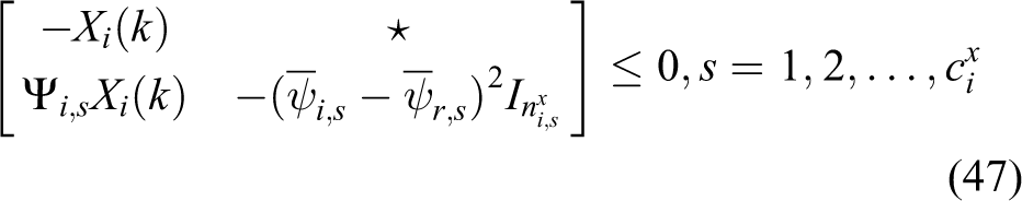
Constraint (15): Define $X_i(k)={\epsilon }_i(k)P_i^{-1}(k)\text{ and }{Y}_i(k)=K_i(k)X_i(k)$ . The constraint (15) can be reformulated as $\parallel x_{ir}(N|k){\parallel }_{X_i^{-1}(k)}^2=x_{ir}^{\text{T}}(N|k)X_i^{-1}(k)x_{ir}(N|k)\le 1$ , which by applying Schur complement is equivalent to

$\left[\begin{array}{cc}-1& \star \\ x_{ir}\left(N|k\right)& -X_i\left(k\right)\end{array}\right]\le 0$

45

Constraint (16): By implementing the terminal control input $u_i^K(t|k)=K_i(k)x_{ir}^K(t|k)+F_{ir}^u(u_r(k+t))$ , the constraint (16) can be guaranteed by ${(A+B{K}_i(k))}^{\text{T}}{P}_i(k)(A+B{K}_i(k))-P_i(k)+\overline{\lambda }(\overline{Q})I_{2n_i}+K_i^{\text{T}}(k)R_i{K}_i(k)\le 0$ , which by applying Schur complement and congruent transformation is equivalent to

$\left[\begin{array}{cccc}-X_i\left(k\right)& \star & \star & \star \\ A{X}_i\left(k\right)+B{Y}_i\left(k\right)& -X_i\left(k\right)& \star & \star \\ X_i\left(k\right)& 0& -\frac{{\epsilon }_i\left(k\right)}{\overline{\lambda }(\overline{Q})}{I}_{2n_i}& \star \\ Y_i\left(k\right)& 0& 0& -\frac{{\epsilon }_i\left(k\right)}{{\rho }_i}{I}_{m_i}\end{array}\right]\le 0$

46

Note that, applying the LMIs (45) and (46) yields $\parallel x_{ir}^K(t|k){\parallel }_{X_i^{-1}(k)}^2\le 1\text{ for all }t\ge N$ .

Constraint (17): Using the triangle inequality, the constraint (17), that is, $\parallel {\Psi }_{i,s}{x}_i^K(t|k)\parallel =\parallel {\Psi }_{i,s}[x_{ir}^K(t|k)+(F_{ir}^x(x_r(k+t))+d_{ir}^x)]\parallel \le {\overline{\psi }}_{i,s}$ , is guaranteed by $\parallel {\Psi }_{i,s}{x}_{ir}^K(t|k)\parallel \le {\overline{\psi }}_{i,s}-{\overline{\psi }}_{r,s}\text{ with }{\overline{\psi }}_{r,s}={{\displaystyle \text{max}}}_{k\ge 0}\parallel {\Psi }_{i,s}(F_{ir}^x(x_r(k))+d_{ir}^x)\parallel$ . Following the property $\parallel x_{ir}^K(t|k){\parallel }_{X_i^{-1}(k)}^2\le 1$ for all t ≥ N, we have $\parallel {\Psi }_{i,s}{x}_{ir}^K(t|k)\parallel =\parallel {\Psi }_{i,s}{X}_i^{1/2}(k)X_i^{-1/2}(k)x_{ir}^K(t|k)\parallel \le \parallel {\Psi }_{i,s}{X}_i^{1/2}(k)\parallel$ for all t ≥ N. Hence, the constraint (17) is guaranteed by $\parallel {\Psi }_{i,s}{X}_i^{1/2}(k)\parallel \le {\overline{\psi }}_{i,s}-{\overline{\psi }}_{r,s}\text{ for all }s=1,\dots ,c_i^x$ , which by applying Schur complement is guaranteed by

$\left[\begin{array}{cc}-X_i\left(k\right)& \star \\ {\Psi }_{i,s}{X}_i\left(k\right)& -{({\overline{\psi }}_{i,s}-{\overline{\psi }}_{r,s})}^2{I}_{n_{i,s}^x}\end{array}\right]\le 0,s=1,2,\dots ,c_i^x$

47

Constraint (18): Similar to the above procedure, the constraint (18) is guaranteed by

$\left[\begin{array}{cc}-X_i\left(k\right)& \star \\ {\Phi }_{i,s}{Y}_i\left(k\right)& -{({\overline{\phi }}_{i,s}-{\overline{\phi }}_{r,s})}^2{I}_{m_{i,s}^u}\end{array}\right]\le 0,s=1,2,\dots ,c_i^u$

48

where ${\overline{\phi }}_{r,s}={{\displaystyle \text{max}}}_{k\ge 0}\parallel {\Phi }_{i,s}{F}_{ir}^u(u_r(k))\parallel$ .

Auxiliary constraint (36): Define ${\theta }_i(k)={\eta }_i^{-1}(k)\text{ and }{x}_{ir}^{{\mathbb{N}}^{+}}=[x_{ir}(1|k);\dots ;x_{ir}(N-1|k)]\in {ℝ}^{2(N-1)n_i}$ . The constraint (36) by applying Schur complement is equivalent to

$\left[\begin{array}{cc}-\frac{\delta {\theta }_i(k)\parallel z_{ir}(k){\parallel }_{Q_i(k)}^2}{2{\Delta }_i}& \star \\ x_{ir}^{{\mathbb{N}}^{+}}& -I_{2(N-1)n_i}\end{array}\right]\le 0$

49

Cost function (37): Define $u_{ir}^{\mathbb{N}}=[u_{ir}(0|k);\dots ;u_{ir}(N-1|k)]\in {ℝ}^{N{m}_i},{\widehat{x}}_{ij}^{{\mathbb{N}}^{+}}=[{\widehat{x}}_{ij}(1|k);\dots ;{\widehat{x}}_{ij}(N-1|k)]\in {ℝ}^{2(N-1)n_i}\text{ and }{\widehat{x}}_{i,{\mathbb{N}}_i(k)}^{{\mathbb{N}}^{+}}=[{\widehat{x}}_{ij}^{{\mathbb{N}}^{+}};\cdots ;{\widehat{x}}_{il}^{{\mathbb{N}}^{+}}]\in {ℝ}^{2(N-1)|{\mathbb{N}}_i(k)|n_i}\text{ with }\{j,\dots ,l\}={\mathbb{N}}_i(k)$ . Let ${\gamma }_i(k)\ge {\displaystyle {\sum }_{t\in \mathbb{N}}}{\rho }_i\parallel u_{ir}(t|k){\parallel }^2+{\displaystyle {\sum }_{t\in \mathbb{N}}}{\displaystyle {\sum }_{j\in {\mathbb{N}}_i(k)}}{\beta }_i(k)\parallel {\widehat{x}}_{ij}(t|k){\parallel }^2={\rho }_i\parallel u_{ir}^{\mathbb{N}}{\parallel }^2+{\beta }_i(k)\parallel {\widehat{x}}_{i,{\mathbb{N}}_i(k)}^{{\mathbb{N}}^{+}}{\parallel }^2$ , which by applying Schur complement is equivalent to

$\left[\begin{array}{ccc}-{\gamma }_i\left(k\right)& \star & \star \\ u_{ir}^{\mathbb{N}}& -{\rho }_i^{-1}{I}_{N{m}_i}& \star \\ {\widehat{x}}_{i,{\mathbb{N}}_i(k)}^{{\mathbb{N}}^{+}}& 0& -{\beta }_i^{-1}\left(k\right)I_{2(N-1)|{\mathbb{N}}_i(k)|n_i}\end{array}\right]\le 0$

50

The cost ${\overline{J}}_i({\epsilon }_i,{\eta }_i,x_{ir},{\widehat{x}}_{i\blacksquare },u_{ir},k)$ can be bounded from above by ${\overline{\overline{J}}}_i\left({\theta }_i,{\gamma }_i,{\epsilon }_i,k\right)=\left(1+\frac{{\alpha }_i\delta {\theta }_i\left(k\right)}{2{\Delta }_i}\right)\parallel z_{ir}\left(k\right){\parallel }_{Q_i(k)}^2+{\gamma }_i\left(k\right)+{\epsilon }_i\left(k\right)$

Optimization problem (38): By incorporating the constraints (43) to (50) and the cost ${\overline{\overline{J}}}_i({\theta }_i,{\gamma }_i,{\epsilon }_i,k)$ , the LMIs optimization problem is formulated as

$\underset{{\epsilon }_i(k),X_i(k),Y_i(k),{\theta }_i(k),{\gamma }_i(k),u_i(t|k),t\in \mathbb{N}}{{\displaystyle \text{min}}}{\overline{\overline{J}}}_i({\theta }_i,{\gamma }_i,{\epsilon }_i,k)\text{\hspace{1em}subject to\hspace{1em}}(43)-(50)$

51

By applying algorithm 1 to each agent $i\in {\mathbb{N}}_a$ by solving the LMIs optimization problem (51), all the properties shown in ‘Property analysis’ section are still guaranteed, which can be similarly verified.

Illustrative examples

To demonstrate the effectiveness and practicability of our result, we provide a comparison and a verification in the following numerical and simulation examples, respectively.

Numerical example

Consider a very simple multi-agent system with ${\mathcal{N}}_a=2$ homogeneous agents ( $i=1,2$ ) in 1D space. The coordinate transform functions are $F_{12}^x(x)=F_{21}^x(x)=I_{2}x$ , and the Lipschitz constants are calculated as ${\overline{F}}_{12}^x={\overline{F}}_{21}^x=1$ . The communication topology is assumed to be time-varying due to the distance between agents, that is, each agent can receive data from the other only for $\parallel d_{12}(k)\parallel =\parallel d_{21}(k)\parallel =\parallel p_1(k)-p_2(k)\parallel \le \overline{d},\text{ where }\overline{d}=5$ denotes the distance limitation of effective communication for each agent. Let us test the monotonous decrease of Lyapunov function, with the fixed formation weighting scalar (as in the literature ^5,13 ) and the real-time updated formation weighting scalars (as in this article).

Give ${\mathbb{N}}_1^0=\left\{2\right\},{\mathbb{N}}_2^0=\left\{1\right\},{\alpha }_1={\alpha }_2={\rho }_1={\rho }_2=1\text{ and }N=2$ and take the convergence speed as $\delta =0.9$ . For comparison, we choose the fixed formation weighting scalars as ${\beta }_1={\beta }_2=2$ and set the upper bounds ${\overline{\beta }}_1={\overline{\beta }}_2=2$ for the real-time updated formation weighting scalars ${\beta }_1(k)\text{ and }{\beta }_2(k)$ .

Suppose the following conditions occur at the instant k

$x_{1r}^{\ast }\left(0|k\right)=[4;2],x_{1r}^{\ast }\left(1|k\right)=[2;1],x_{1r}^{\ast }\left(2|k\right)=[0;0],u_{1r}^{\ast }\left(0|k\right)=-1,u_{1r}^{\ast }\left(1|k\right)=-1$

52

$x_{2r}^{\ast }\left(0|k\right)=-[4;2],x_{2r}^{\ast }\left(1|k\right)=-[2;1],x_{2r}^{\ast }\left(2|k\right)=[0;0],u_{2r}^{\ast }\left(0|k\right)=1,u_{2r}^{\ast }\left(1|k\right)=1$

53

Then, the optimal costs of all agents are calculated as

$\begin{array}{c}{J}_1\left(x_{1r}^{\ast },{\widehat{x}}_{12}^{\ast },u_{1r}^{\ast },k\right)=1\times \left(\parallel [4;2]{\parallel }^2+\parallel [2;1]{\parallel }^2\right)+1\times \left(\parallel -1{\parallel }^2+\parallel -1{\parallel }^2\right)+\parallel [0;0]{\parallel }_{P_1^{\ast }(k)}^2=27\\ J_2\left(x_{2r}^{\ast },{\widehat{x}}_{21}^{\ast },u_{2r}^{\ast },k\right)=1\times \left(\parallel -[4;2]{\parallel }^2+\parallel -[2;1]{\parallel }^2\right)+1\times \left(\parallel 1{\parallel }^2+\parallel 1{\parallel }^2\right)+\parallel [0;0]{\parallel }_{P_2^{\ast }(k)}^2=27\end{array}$

It deserves to note that, because $\parallel d_{12}(k)\parallel =\parallel d_{21}(k)\parallel =\parallel p_{1r}^{\ast }(0|k)-p_{2r}^{\ast }(0|k)\parallel =\parallel 4-(-4)\parallel =8>\overline{d}\text{ induces }{\mathbb{N}}_1(k)={\mathbb{N}}_2(k)=Ø$ , the terms ${\widehat{x}}_{12}(0|k),{\widehat{x}}_{12}(1|k),{\widehat{x}}_{21}(0|k)\text{ and }{\widehat{x}}_{21}(1|k)$ are not incorporated in the real-time costs.

At the instant k + 1, because $\parallel d_{12}(k+1)\parallel =\parallel d_{21}(k+1)\parallel =\parallel p_{1r}^{\ast }(1|k)-p_{2r}^{\ast }(1|k)\parallel =\parallel 2-(-2)\parallel =4<\overline{d}\text{ induces }{\mathbb{N}}_1(k+1)={\mathbb{N}}_1^0\text{ and }{\mathbb{N}}_2(k+1)={\mathbb{N}}_2^0$ , the feasible state and input deviation sequences are obtained, according to case 1 in proof (a) of theorem 5.1 as

$\begin{array}{l}{x}_{1r}^{\circ }\left(0|k+1\right)=x_{1r}^{\ast }\left(1|k\right)=[2;1],x_{1r}^{\circ }\left(1|k+1\right)=x_{1r}^{\ast }(2|k)=[0;0],x_{1r}^{\circ }\left(2|k+1\right)=x_{1r}^K\left(3|k\right)=[0;0]\\ {\widehat{x}}_{12}^{\circ }\left(0|k+1\right)=x_1^{\circ }\left(0|k+1\right)-{\widehat{x}}_2\left(0|k+1\right)=x_{1r}^{\ast }\left(1|k\right)-x_{2r}^{\ast }(1|k)=[4;2],u_{1r}^{\circ }\left(0|k+1\right)=u_{1r}^{\ast }\left(1|k\right)=-1\\ {\widehat{x}}_{12}^{\circ }\left(1|k+1\right)=x_1^{\circ }\left(1|k+1\right)-{\widehat{x}}_2\left(1|k+1\right)=x_{1r}^{\ast }\left(2|k\right)-x_{2r}^{\ast }\left(2|k\right)=[0;0],u_{1r}^{\circ }\left(1|k+1\right))=K_1^{\ast }(k)x_{1r}^{\ast }\left(2|k\right)=0\end{array}$

54

$\begin{array}{c}{x}_{2r}^{\circ }\left(0|k+1\right)=x_{2r}^{\ast }\left(1|k\right)=-[2;1],x_{2r}^{\circ }\left(1|k+1\right)=x_{2r}^{\ast }\left(2|k\right)=[0;0],x_{2r}^{\circ }\left(2|k+1\right)=x_{2r}^K\left(3|k\right)=[0;0]\\ {\widehat{x}}_{21}^{\circ }\left(0|k+1\right)=x_2^{\circ }\left(0|k+1\right)-{\widehat{x}}_1\left(0|k+1\right)=x_{2r}^{\ast }\left(1|k\right)-x_{1r}^{\ast }\left(1|k\right)=-[4;2],u_{2r}^{\circ }\left(0|k+1\right)=u_{2r}^{\ast }\left(1|k\right)=1\\ {\widehat{x}}_{21}^{\circ }\left(1|k+1\right)=x_2^{\circ }\left(1|k+1\right)-{\widehat{x}}_1\left(1|k+1\right)=x_{2r}^{\ast }\left(2|k\right)-x_{1r}^{\ast }(2|k)=[0;0],u_{2r}^{\circ }\left(1|k+1\right)=K_2^{\ast }(k)x_{2r}^{\ast }\left(2|k\right)=0\end{array}$

55

With the fixed formation weighting scalars ${\beta }_1={\beta }_2=2$ , the associated feasible costs of all agents are calculated as

$\begin{array}{c}{J}_1\left(x_{1r}^{\circ },{\widehat{x}}_{12}^{\circ },u_{1r}^{\circ },k+1\right)=1\times \left(\parallel [2;1]{\parallel }^2+\parallel [0;0]{\parallel }^2\right)+1\times \left(\parallel -1{\parallel }^2+\parallel 0{\parallel }^2\right)+2\times \left(\parallel [4;2]{\parallel }^2+\parallel [0;0]{\parallel }^2\right)+\parallel [0;0]{\parallel }_{P_1^{\ast }(k)}^2=46\\ J_2\left(x_{2r}^{\circ },{\widehat{x}}_{21}^{\circ },u_{2r}^{\circ },k+1\right)=1\times \left(\parallel -[2;1]{\parallel }^2+\parallel [0;0]{\parallel }^2\right)+1\times \left(\parallel 1{\parallel }^2+\parallel 0{\parallel }^2\right)+2\times \left(\parallel -[4;2]{\parallel }^2+\parallel [0;0]{\parallel }^2\right)+\parallel [0;0]{\parallel }_{P_2^{\ast }(k)}^2=46\end{array}$

which yield $V(k+1)-V(k)\le {\displaystyle {\sum }_{i=1}^2}{J}_i(x_{ir}^{\circ },{\widehat{x}}_{i\blacksquare }^{\circ },u_{ir}^{\circ },k+1)-{\displaystyle {\sum }_{i=1}^2}{J}_i(x_{ir}^{\ast },{\widehat{x}}_{i\blacksquare }^{\ast },u_{ir}^{\ast },k)\le (46+46)-(27+27)=38$ . Hence, the guarantee for the monotonous decrease of the Lyapunov function may be lost.

By applying algorithm 1, the conditions (52) and (53) yield (according to the condition (40))

${\eta }_i^{\ast }\left(k\right)=\frac{\delta \parallel z_{ir}\left(k\right){\parallel }_{Q_i(k)}^2}{2{\Delta }_i\sum _{t=1}^{N-1}\parallel x_{ir}^{\ast }\left(t|k\right){\parallel }^2}=\frac{0.9\times 20}{2\times 2\times 5}=0.9,i=1,2,$

56

and ${\beta }_1(k+1)={\beta }_2(k+1)=0.9$ (according to the update equation (34)). Then, the feasible costs of all agents at the instant k + 1 are calculated as

$\begin{array}{c}{J}_1\left(x_{1r}^{\circ },{\widehat{x}}_{12}^{\circ },u_{1r}^{\circ },k+1\right)=1\times \left(\parallel [2;1]{\parallel }^2+\parallel [0;0]{\parallel }^2\right)+1\times \left(\parallel -1{\parallel }^2+\parallel 0{\parallel }^2\right)+0.9\times \left(\parallel [4;2]{\parallel }^2+\parallel [0;0]{\parallel }^2\right)+\parallel [0;0]{\parallel }_{P_1^{\ast }(k)}^2=24\\ J_2\left(x_{2r}^{\circ },{\widehat{x}}_{21}^{\circ },u_{2r}^{\circ },k+1\right)=1\times \left(\parallel -[2;1]{\parallel }^2+\parallel [0;0]{\parallel }^2\right)+1\times \left(\parallel 1{\parallel }^2+\parallel 0{\parallel }^2\right)+0.9\times \left(\parallel -[4;2]{\parallel }^2+\parallel [0;0]{\parallel }^2\right)+\parallel [0;0]{\parallel }_{P_2^{\ast }(k)}^2=24\end{array}$

These lead to $V(k+1)-V(k)\le (24+24)-(27+27)=-6$ , that is, the monotonous decrease of the Lyapunov function is strictly guaranteed.

Simulation example

Consider a simultaneous tracking and formation problem of nonhomogeneous multi-agents with ${\mathcal{N}}_a=6$ vehicles in 3D space. The vehicles are composed of three 2D vehicles and three 3D vehicles, whose dynamics are formulated as in equation (1) with the parameters $A_i=\left[\begin{array}{cc}{I}_2& I_2\\ 0& I_2\end{array}\right]\text{ and }{B}_i=\left[\begin{array}{c}0.5I_2\\ I_2\end{array}\right]\text{ for }i=1,2,3\text{ and }{A}_i=\left[\begin{array}{cc}{I}_3& I_3\\ 0& I_3\end{array}\right]\text{ and }{B}_i=\left[\begin{array}{c}0.5I_3\\ I_3\end{array}\right]\text{ for }i=4,5,6$ . These dynamics models are obtained by discretizing the associated continuous-time models with sampling period 1 s. The initial states of these vehicles are given as $x_1(0)=[0;-7.5;0;0],x_2(0)=[0;4.5;0;0],x_3(0)=[0;-1.5;0;0],x_4(0)=[0;-4.5;0;0;0;0],x_5(0)=[0;7.5;0;0;0;0]\text{ and }{x}_6=[0;1.5;0;0;0;0]$ .

The velocity and acceleration (i.e. input) constraints are desired for each vehicle $i\in {\mathbb{N}}_a\text{ as }\parallel v_i(k)\parallel \le {\overline{v}}_i\text{ and }\parallel u_i(k)\parallel \le {\overline{u}}_i$ , with the upper bounds ${\overline{v}}_i=\sqrt{2}\text{ and }{\overline{u}}_i=0.2$ . Additionally, the vertical acceleration constraint of 3D vehicles are desired as $\parallel u_{i\mathrm{,3}}(k)\parallel \le {\overline{u}}_v\text{ for }i=4,5,6$ , with the upper bounds ${\overline{u}}_v=0.05$ . By reformulating the above constraints according to equations (2) and (3), we can obtain the constraint parameters as ${\Psi }_i=\{\begin{array}{ll}[0,I_2]\in {ℝ}^{2\times 4},\hfill & i=1,2,3\hfill \\ [0,I_3]\in {ℝ}^{3\times 6},\hfill & i=4,5,6\hfill \end{array},{\Phi }_{i\mathrm{,1}}=\{\begin{array}{ll}{I}_2,\hfill & i=1,2,3\hfill \\ I_3,\hfill & i=4,5,6\hfill \end{array},{\overline{\psi }}_i=\sqrt{2}\text{ and }{\overline{\phi }}_{i\mathrm{,1}}=0.2\text{ for }i\in {\mathbb{N}}_a,{\Phi }_{i\mathrm{,2}}=[0,0,1]\text{ and }{\overline{\phi }}_{i\mathrm{,2}}=0.05\text{ for }i=4,5,6$ .

The reference agent is a virtual vehicle with the same dynamic equation with the 2D vehicles, whose initial state and control input are given as $x_r(0)=[0;0;0;0]\text{ and }{u}_r(k)=[u_{r\mathrm{,1}}(k);u_{r\mathrm{,2}}(k)]=[{\overline{u}}_r\text{cos}(0.1k);{\overline{u}}_r\text{cos}(0.25k)]\text{ with }{\overline{u}}_r=0.1$ . The desired tracking and formation vectors are given as $d_{1r}^p=[2;0],d_{2r}^p=[-2;-2],d_{3r}^p=[-2;2],d_{4r}^p=[-2;0;4],d_{5r}^p=[4;-2;4],d_{6r}^p=[3;2;4],d_{12}^p=[4;2],d_{13}^p=[4;-2],d_{15}^p=[0;2],d_{16}^p=[0;-2],d_{21}^p=[-4;-2],d_{23}^p=[0;-4],d_{24}^p=[0;-2],d_{31}^p=[-4;2],d_{32}^p=[0;4],d_{34}^p=[0;2],d_{42}^p=[0;2;4],d_{43}^p=[0;-2;4],d_{45}^p=[-4;2;0],d_{46}^p=[-4;-2;0],d_{51}^p=[0;-2;4],d_{54}^p=[4;-2;0],d_{56}^p=[0;-4;0],d_{61}^p=[0;2;4],d_{64}^p=[4;2;0]\text{ and }{d}_{65}^p=[0;4;0]$ .

In this simulation, the scalars ${\alpha }_i=1,{\rho }_i=1\text{ and }{\overline{\beta }}_i=1$ are given for each vehicle $i\in {\mathbb{N}}_a$ ; the scalars δ = 0.99 and N = 5 are chosen for all vehicles. According to the dynamics of these vehicles, the coordinate transformation functions can be determined as $F_{ir}^x(x)=\{\begin{array}{ll}{I}_{4}x,\hfill & i=1,2,3\hfill \\ \text{diag}\{[I_2;0],[I_2;0]\}x,\hfill & i=4,5,6\hfill \end{array},F_{ir}^u(u)=\{\begin{array}{ll}{I}_{2}u,\hfill & i=1,2,3\hfill \\ [I_2;0]u,\hfill & i=4,5,6\hfill \end{array}\text{,and\hspace{0.17em}}{F}_{ij}^x(x)=\{\begin{array}{ll}\text{diag}\{[I_2\mathrm{,0}],[I_2\mathrm{,0}]\}x,\hfill & i=1,2,3\text{\hspace{0.17em}and }j=4,5,6\hfill \\ \text{diag}\{[I_2;0],[I_2;0]\}x,\hfill & i=4,5,6\text{\hspace{0.17em}and }j=1,2,3\hfill \\ I_{4}x,\hfill & i,j=1,2,3;\hfill \\ I_{6}x,\hfill & i,j=4,5,6,\hfill \end{array}$ ,

following which the Lipschitz constants can be calculated as ${\overline{F}}_{ij}^x=1\text{ for all }(i,j)\in \mathbb{F}$ . The parameters $\overline{\lambda }(\overline{Q})\approx 13,{\Delta }_i=8\text{ for }i=1,4\text{ and }{\Delta }_i=6\text{ for }i=2,3,5,6$ can be calculated. The communication topology is time-varying due to the distance limitation of effective communication, which is set as $\overline{d}=5$ for all vehicles. Note that, the communications between some desired pairs of vehicles fail at the initial instant, since the distances between these desired pairs are greater than $\overline{d}$ . Table 2 shows the real-time neighbourhood of vehicles over the simulation horizon.

Table 2.

Real-time neighbour index sets of all vehicles.

Instant k	0	1	2	3	4	5	6	7	8	9	10	11	12–30
${\mathbb{N}}_1(k)$	Ø	Ø	Ø	Ø	Ø	Ø	Ø	{2}	{2}	{2,5}	{2,5}	{2,5,6}	{2,3,5,6}
${\mathbb{N}}_2(k)$	Ø	Ø	Ø	{3}	{3}	{3,4}	{3,4}	{1,3,4}	{1,3,4}	{1,3,4}	{1,3,4}	{1,3,4}	{1,3,4}
${\mathbb{N}}_3(k)$	{4}	{4}	{4}	{2,4}	{2,4}	{2,4}	{2,4}	{2,4}	{2,4}	{2,4}	{2,4}	{2,4}	{1,2,4}
${\mathbb{N}}_4(k)$	{3}	{3}	{3}	{3}	{3}	{2,3}	{2,3}	{2,3,5,6}	{2,3,5,6}	{2,3,5,6}	{2,3,5,6}	{2,3,5,6}	{2,3,5,6}
${\mathbb{N}}_5(k)$	Ø	Ø	Ø	{6}	{6}	{6}	{6}	{4,6}	{4,6}	{1,4,6}	{1,4,6}	{1,4,6}	{1,4,6}
${\mathbb{N}}_6(k)$	Ø	Ø	Ø	{5}	{5}	{5}	{5}	{4,5}	{4,5}	{4,5}	{4,5}	{1,4,5}	{1,4,5}

By applying algorithm 1 by solving the optimization problem (51), we simulate this example through MATLAB on a PC with a dual-core 3.2 GHz Intel i5 CPU and a 3.47 GB RAM. Over the simulation horizon, all the optimal solutions are solved and implemented at each instant for each vehicle, that is, the recursive feasibility of the optimization problem (51) is demonstrated. Because the optimization problem (51) is an equivalent LMIs version of the optimization problem (38), the conclusion (a) of theorem 5.1 is verified. According to the solved solutions, the left and right terms of equation (39) are calculated and shown in Figure 1. It can be easily seen that the values of both sides in equation (39) are always identical for each vehicle; hence, the equality (39) is verified. Similarly, Figure 2 verifies the equality (40). These further verify the conclusion (b) of theorem 5.1 following the proof by contradiction. With the implementation of the solved solutions, the values of each vehicle’s real-time cost and the global cost are calculated and depicted in Figure 4. The monotonous decrease of the global cost verifies the conclusion (c) of theorem 5.1. More detailed simulation results are provided with analysis in the following.

Figure 1.

The left and right terms of equation (39), where ${\text{Lt}}_i(k)=\parallel x_{ir}^{\ast }(N|k){\parallel }_{P_i^{\ast }(k)}^2\text{ and }{\text{Rt}}_i(k)={\epsilon }_i^{\ast }(k)$ .

Figure 2.

The left and right terms of equation (40), where ${\text{Lt}}_i(k)={\displaystyle {\sum }_{t\in \mathbb{N}}}\parallel x_{ir}^{\ast }(t|k){\parallel }^2\text{ and }{\text{Rt}}_i(k)=\frac{\delta }{2{\eta }_i^{\ast }(k){\Delta }_i}\parallel z_{ir}(k){\parallel }_{Q_i(k)}^2$ .

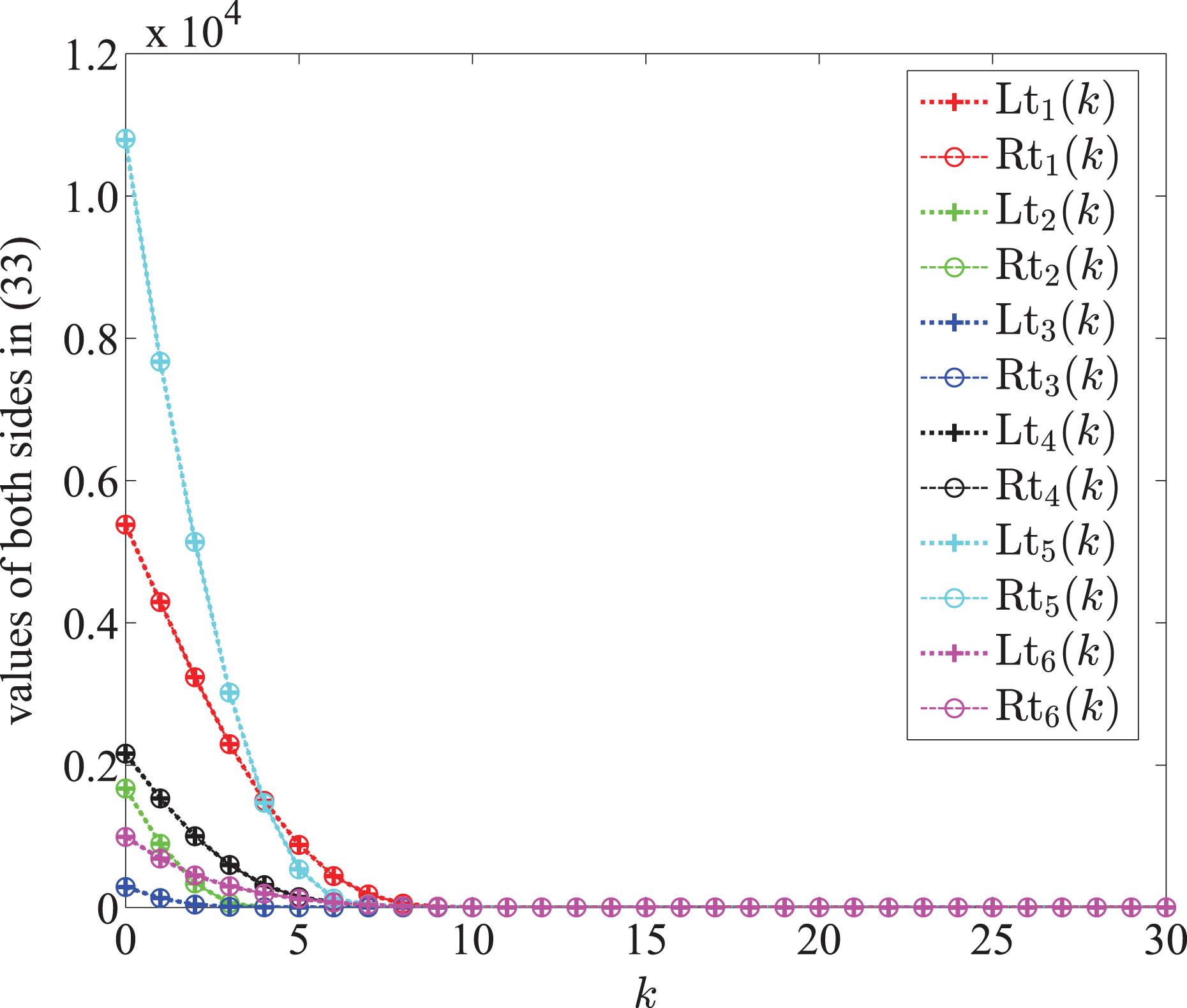
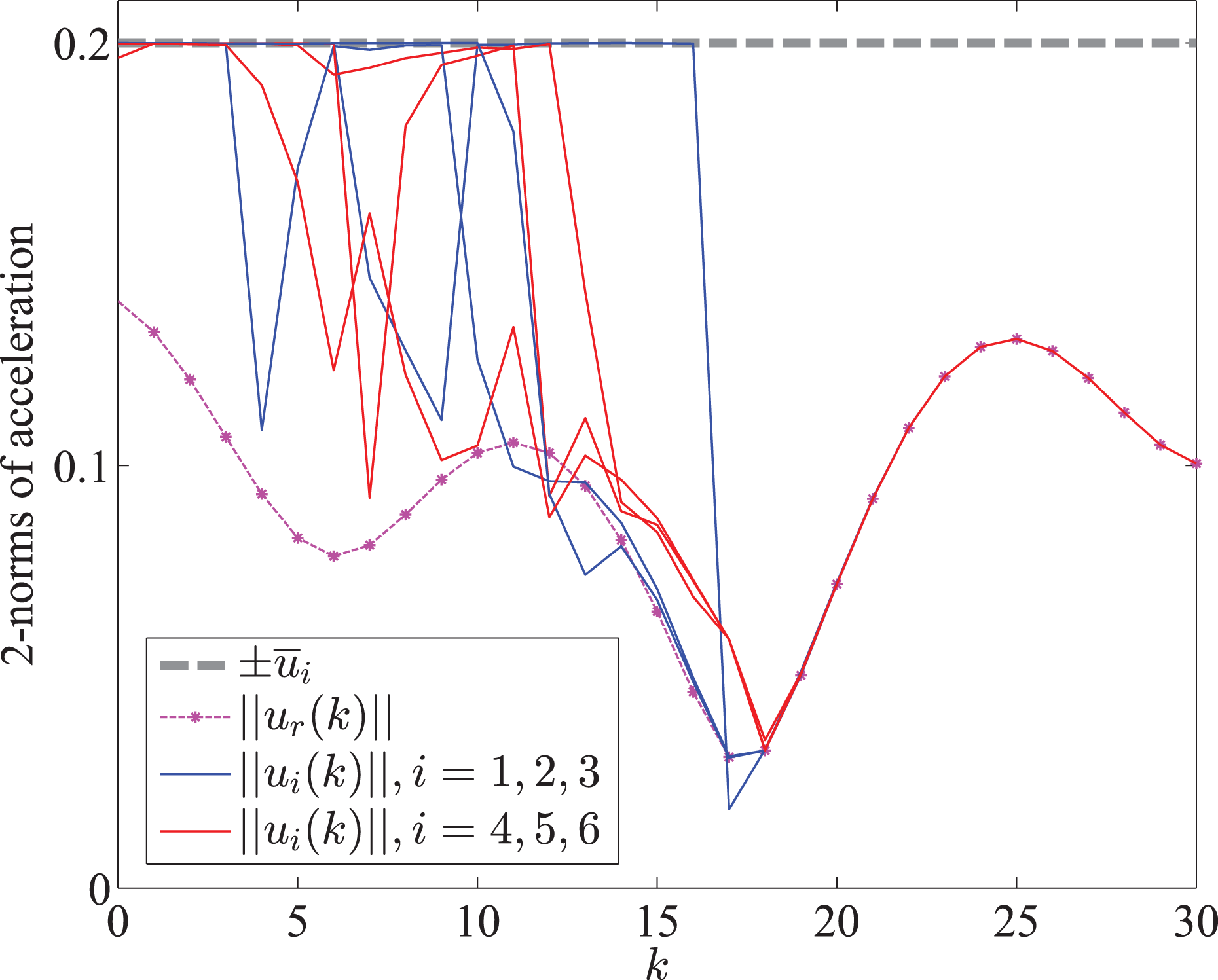
In Figure 3, the simulation trajectories of all vehicles and reference object are depicted, where the initial and final positions of all vehicles and reference object are marked with indices, and the desired formation is denoted by black dashed lines. It can be easily seen that all the 2D and 3D vehicles successfully track the reference object and achieve the desired formation, although the communication topology is time-varying. Additionally, the velocities and accelerations of all vehicles converge to those of the reference object (see Figures 5 to 7), which means that the vehicles will keep the desired tracking and formation in future. In Figures 5 to 7, the two-norms of all vehicles’ velocities do not exceed ${\overline{v}}_i=\sqrt{2}$ , the two-norms of all vehicles’ inputs (i.e. accelerations) do not exceed ${\overline{u}}_i=0.2$ and the vertical accelerations of 3D vehicles $i=4,5,6$ do not exceed the range $[-0.05,0.05]$ . These mean that all the desired state and input constraints are not violated over the simulation horizon. Thus, the effectiveness and practicability of the proposed DRHC strategy are illustrated.

Figure 3.

The trajectories of vehicles and reference object.

Figure 4.

The values of the cost functions.

Figure 5.

The two-norms of velocities.

Figure 6.

The two-norms of accelerations.

Figure 7.

The vertical accelerations of 3D vehicles.

To further verify the purpose discussed in ‘Implementation of DRHC strategy’ section (see the first paragraph after algorithm 1), we depict the update trends of the formation weighting scalars ${\beta }_i(k)$ s in Figure 8. It can be easily found that minimizing ${\overline{J}}_i({\epsilon }_i,{\eta }_i,x_{ir},{\widehat{x}}_{i\blacksquare },u_{ir},k)$ tends to solve large ${\eta }_i(k)$ s and then to update large formation weighting scalars ${\beta }_i(k)$ s. For the real-time implementation, we show the optimization times $T{c}_i(k)$ of each vehicle $i\in {\mathbb{N}}_a$ in Figure 9. Note that, all the optimization times are smaller than the sampling period 1 s; hence, a real-time implementation can be simulated by solving in advance a predictive version of the optimization problem (51) at each instant k − 1 (more details refer to the second paragraph after algorithm 1). Because the simulation results are similar to those provided above, the detailed graphs of the simulation trajectories, costs, velocities and accelerations are omitted here.

Figure 8.

The real-time formation weighting scalars.

Figure 9.

The optimization times of all vehicles.

Conclusion

For the simultaneous tracking and formation problem of nonhomogeneous multi-agents with time-varying communication topology, we study the synthesis of DRHC in this article. By considering the control objective and real-time communication topology, we generate the individual cost function for each agent online, design an auxiliary constraint in distributed form and impose it in the optimization problem and propose an update equation for the formation weighting parameter. Accordingly, the individual optimization problem and associated DRHC algorithm are presented. By applying the presented DRHC algorithm, the recursive feasibility of the optimization problem and the exponential stability (i.e. the exponential convergence of tracking and formation) of the overall multi-agent system are guaranteed. Due to the handling of the effects of the time-varying communication topology on the recursive feasibility and stability, our result is preferred for miscellaneous practical applications.

Indeed, the practical application of nonhomogeneous multi-agents involves more factors, such as the collision avoidance, obstacle avoidance, formation switching, disturbance handling and so on, which will arouse a series of theoretical issues to be considered in our future researches.