Generalized dynamic model and control of ambiguous mono axial vehicle robot

Abstract

This article deals with the novel concept of ambiguous mono axial vehicle robot. Such robot is a combination of Segway and dicycle, which utilizes the advantages of each chassis. The advantage of dicycle is lower energy consumption during the movement and the higher safety of carried payload. The movable platform inside the ambiguous mono axial vehicle allows using the various sensors or devices. This will change the ambiguous mono axial vehicle to the Segway type robot. Both these modes are necessary to control in the stable mode to ensure the safety of the ambiguous mono axial vehicle’s movement. The main contents of the article contain description of generalized dynamic model of ambiguous mono axial vehicle and related control of ambiguous mono axial vehicle. The proposal is unique in that the same controller is used for both modes. Several simulations verify proposed control schemes and identified parameters. Moreover, the dicycle type of platform has never been used in robotics and that is another novelty.

Introduction

Many constructions of two-wheeled differential robots without any supporting wheels appeared after introduction of Segway™ in December 2001. ¹ Significant characteristic of this chassis is that the gravity center is high above wheels axis, and therefore it is needed to actively control the chassis. ² The research on balancing two-wheeled robots is very strong in recent years. This is due to that the control consists not only from control of required motion, but it includes also the stability control of inherent unstable system. After introduction of Segway, a lot of similar chassis appeared. The idea of balancing such chassis is based on the concept of inverted pendulum. As an example of the mobile-inverted pendulum, JOE robot can be mentioned. ³ Control of this chassis was solved by pole placement using state feedback controller. Other similar chassis were constructed as simple demonstrational chassis. ⁴ Another had more complicated chassis used for mobile robots. ⁵ The simpler constructions used feedback control of angle of inclination by Proportional Derivative (PD) controller. In these solutions, parameters of controller were not so much analyzed. PD controller was usually adjusted only by estimation. The reason of not using integral parameter “I” is stated in the study by Sridharan and Zoghi, ⁶ as its demand of large amount of processing power. Complex solutions were based on the thoroughgoing analysis of dynamical and state model. These solutions used for example state feedback control by Linear Quadratic Regulator (LQR) controller, ^2,7 sliding mode control, ⁸ fuzzy LQR control, ⁹ or fuzzy PD-like control. ^10,11 Most of the mentioned works validated only the controllability of the chassis. One of the most important contributions discussing the dynamics of inverted pendulum robot is the work done by Kim et al. ¹² All of these works analyzed only differential two-wheeled chassis ¹³ with the gravity center above the wheels’ axis. Such construction is advantageous when the payload is above the axis. However, this is disadvantageous for the safety of payload during the transport. Therefore, it is needed to analyze dicycle and to transfer this knowledge into the control of ambiguous mono axial vehicle (AMAV).

In the case of dicycle, the body is smaller than wheels’ diameter. This makes the body protected from the potential collisions during the flips. Moreover, dicycle has the gravity center under wheels axis. Due to this, it is not needed to solve the stabilization of this chassis during the movement. On the contrary, it is needed to solve damping of oscillations, which are excited due the changes in the movement or due to external disturbances. Such constructions were used only as hobby transport vehicles ¹⁴ and they have never been used in mobile robotics. For this reason, our proposed concept is innovative and it can be considered as prototype of such chassis in mobile robotics.

The advantages of two-wheeled differential drive ¹⁵ of any type are the lower energy consumption compared to other wheeled drives and its high dexterity. If this chassis is used in structured environment with narrow surface, the usage of odometry is much more accurate than in the case of slipping controlled chassis. On the basis of this, new concept of two-wheeled differential robot was proposed. This concept combines Segway and dicycle into one chassis (Figure 1).

Figure 1.

Ambiguous mono axial vehicle.

The basis of this structure is that diameter of used wheels is bigger than the body. This is similar to dicycle. However, structure also contains movable platform, which allows the pushing out of payload above wheels axis. This is similar to Segway. This is significantly changing the parameters of the vehicle (or more precisely the center of gravity), as it can be seen in Figure 2.

Figure 2.

The change of CG’s position after the payload is pushed out of moving platform. CG: center of gravity.

This hybrid vehicle can hide useful device in retracted position. As a consequence, vehicle has less energy consumption during the transport. In the case that the useful device (camera or other sensor unit needed to be hold in certain height above the ground during its operation) should be used, it can be pushed out by movable platform. Consequently, the vehicle becomes unstable and the energy consumption increases. However, this uplift is not so significant like it is in the Segway chassis. The chassis is designed to adapt the changes in real time during any type of movement.

If the movable platform is inside the body, the center of gravity is under wheels axis. Behavior of the vehicle will be similar to dicycle. Therefore, it will be equivalent to system of pendulum hung on the wheels axis. Vehicle will be stable, but it will tend to oscillate. These oscillations are excited by the changes in movement (velocity) or external disturbances. If the movable platform is pushed out, the center of gravity is above wheels axis. Behavior of the vehicle will be similar to Segway. It will be equivalent to inverted pendulum hung on the wheels axis. In this case, the vehicle is unstable and it tends to flip forward or backward. This must be compensated by suitable control. It is clear that this hybrid vehicle can operate in two modes and both modes must be reliably controlled.

The article is organized as follows: section “Kinematics of AMAV” describes the kinematics of AMAV based on standard two-wheeled robot kinematics. Section “Dynamics of AMAV” analyzes the dynamics with Lagrange equations of the second kind. Section “Simulations” verifies the proposed model for stable (dicycle) and unstable (Segway) mode. Consequently, in section “Generalized dynamic model of AMAV,” the generalized model of AMAV is derived. Finally, in section “Synthesis of control,” the control of such vehicle is proposed and verified.

Kinematics of AMAV

Kinematics of AMAV is similar to classical differential two-wheeled drive (Figure 3). The movement of the AMAV is controlled by the change of rotational speeds of individual drives. Center of gravity (CG) is in the middle of the wheels axis. Distance D is the half of the wheels distance, R is the wheel radius, v _L and v _R are the velocities of wheels, and v _T is the velocity of CG. CG is defined by the coordinates x _T and y _T. Angle Ψ defines the rotation of the vehicle, more precisely this angle is defined as the angle between v _T and axis x.

Figure 3.

Kinematics of AMAV. AMAV: ambiguous mono axial vehicle.

The following relations define the kinematics of AMAV ¹⁶

$v_{\text{T}}=\frac{v_{\text{L}}+v_{\text{R}}}{2}$

1

$\dot{\psi }=\frac{v_{\text{L}}-v_{\text{R}}}{D}$

2

The velocity of CG in particular axis is defined

$v_{\text{TX}}=\frac{v_{\text{L}}+v_{\text{R}}}{2}.\cos \psi$

3

$v_{\text{TY}}=\frac{v_{\text{L}}+v_{\text{R}}}{2}.\text{sin}\psi$

4

Dynamics of AMAV

There is an assumption that the mass of the AMAV is symmetrical. Therefore, the kinematics will influence dynamic behavior of the system in a very small way. Body of AMAV may be replaced by the inverted pendulum hung on the wheels axis (Figure 4). Wheels axis also defines the rotational linkage between the wheels and AMAV body.

Figure 4.

Substitution of AMAV by inverted pendulum. AMAV: ambiguous mono axial vehicle.

Such model is described by parameters defined in Figure 5: m _w represents the wheels weight, J _w is the moment of inertia, R is the wheel radius, l is the pendulum length, θ is the deflection angle, and m _p is the pendulum weight.

Figure 5.

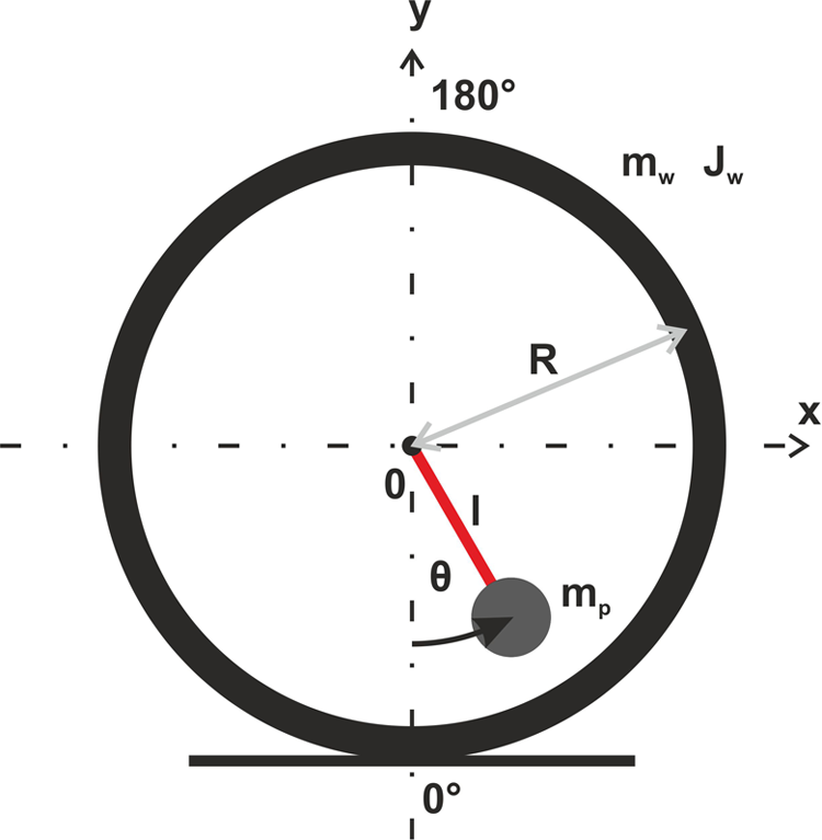
AMAV, its parameters, and coordinate system. AMAV: ambiguous mono axial vehicle.

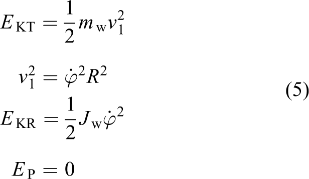
First, the external forces (driving and damping forces) will not be considered to derive the dynamics of AMAV. Differential equations, which describe the dynamics of AMAV, can be defined by the usage of Lagrange equations of the second kind. Kinetic (translational and rotational) and potential energy of the wheel is defined

$\begin{array}{l}{E}_{\text{KT}}=\frac{1}{2}{m}_{\text{w}}{v}_1^2\\ v_1^2={\stackrel{\text{.}}{\varphi }}^2{R}^2\\ E_{\text{KR}}=\frac{1}{2}{J}_{\text{w}}{\stackrel{\text{.}}{\varphi }}^2\\ E_{\text{P}}=0\end{array}$

5

$\dot{\varphi }$ defines the angular velocity of wheel. Kinetic and potential energy of the body is defined

$\begin{array}{l}{E}_{\text{K}}=\frac{1}{2}{m}_{\text{p}}{v}_{\text{T}}^2\\ v_{\text{T}}^2=v_{\text{TX}}^2+v_{\text{TY}}^2\\ v_{\text{TX}}=\frac{\text{d}}{\text{d}t}\left(x+l\text{sin}\left(\theta \right)\right)=\dot{x}+l.\cos \left(\theta \right)\dot{\theta }\\ \dot{x}=\dot{\varphi }.R\\ v_{\text{TY}}=\frac{\text{d}}{\text{d}t}\left(-l\cos \left(\theta \right)\right)=-l\text{sin}\left(\theta \right)\dot{\theta }\end{array}$

6

$\begin{array}{l}{v}_{\text{T}}^2={\dot{\varphi }}^2{R}^2+2\dot{\varphi }Rl\cos \left(\theta \right)\theta \dot{}+l^2{\cos }^2\left(\theta \right){\theta \dot{}}^2+l^2{\text{sin}}^2\left(\theta \right){\dot{\theta }}^2\\ l^2{\cos }^2\left(\theta \right){\dot{\theta }}^2+l^2{\text{sin}}^2\left(\theta \right){\dot{\theta }}^2=l^2{\dot{\theta }}^2\\ E_{\text{K}}=\frac{1}{2}{m}_{\text{p}}{\dot{\varphi }}^2{R}^2+m_{\text{p}}lR\dot{\varphi }\cos \left(\theta \right)\dot{\theta }+\frac{1}{2}{m}_{\text{p}}{l}^2{\dot{\theta }}^2\\ E_{\text{P}}=m_{\text{p}}gl\left(1-\cos \left(\theta \right)\right)\end{array}$7

Lagrangian of AMAV is defined

$L=T-U$

8

Where T is the kinetic energy of AMAV and U is the potential energy of AMAV. Therefore, the Lagrangian of AMV is described by equation

$L=\frac{1}{2}{\dot{\varphi }}^2{R}^2\left(m_{\text{p}}+m_{\text{w}}\right)+\frac{1}{2}{J}_{\text{w}}{\dot{\varphi }}^2+m_{\text{p}}lR\dot{\varphi }\cos \left(\theta \right)\dot{\theta }+\frac{1}{2}{m}_{\text{p}}{l}^2{\dot{\theta }}^2-m_{\text{p}}gl\left(1-\cos \left(\theta \right)\right)$

9

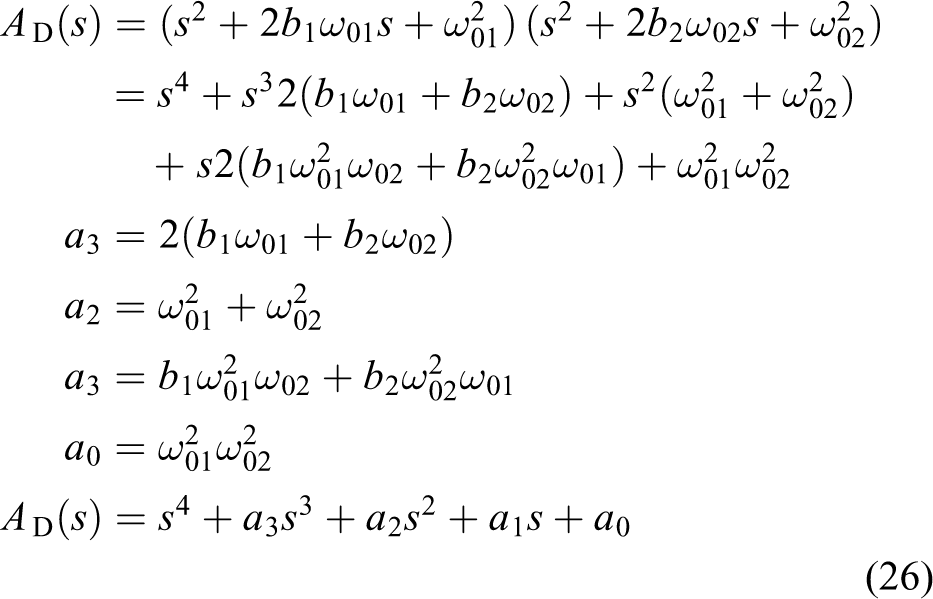
It is clear that these parameters describe the coordinates of the system:

$\varphi ,\dot{\varphi },\text{\hspace{0.17em}and}\stackrel{\text{..}}{\varphi }$ angular position, velocity, and acceleration of the wheel

$\theta ,\dot{\theta },\text{\hspace{0.17em}and\hspace{0.17em}}\stackrel{\text{..}}{\theta }$ angular position, velocity, and acceleration of the body

The equations, which describe the dynamics of AMAV, are defined as Lagrange equations of the second kind

$\frac{\text{d}}{\text{d}t}\left(\frac{\partial L}{\partial \dot{\varphi }}\right)-\frac{\partial L}{\partial \varphi }=0$

10

$\frac{\text{d}}{\text{d}t}\left(\frac{\partial L}{\partial \dot{\theta }}\right)-\frac{\partial L}{\partial \theta }=0$

11

Individual members of equations are defined

$\begin{array}{l}\frac{\partial L}{\partial \varphi }=0\\ \frac{\text{d}}{\text{d}t}\left(\frac{\partial L}{\partial \dot{\varphi }}\right)=\left(m_{\text{w}}{R}^2+m_{\text{p}}{R}^2+J_{\text{w}}\right)\dot{\varphi }\\ +m_{\text{p}}lR\left(\cos \left(\theta \right)\stackrel{\text{..}}{\theta }-{\dot{\theta }}^2\text{sin}\left(\theta \right)\right)\\ \frac{\partial L}{\partial \theta }=-m_{\text{p}}lR\dot{\varphi }\dot{\theta }\text{sin}\left(\theta \right)-m_{\text{p}}gl\text{sin}\left(\theta \right)\\ \frac{\text{d}}{\text{d}t}\left(\frac{\partial L}{\partial \dot{\theta }}\right)=m_{\text{p}}lR\left(\stackrel{\text{..}}{\varphi }\cos \left(\theta \right)-\dot{\theta }\dot{\varphi }\text{sin}\left(\theta \right)\right)+m_{\text{p}}{l}^2\stackrel{\text{..}}{\theta }\end{array}$

12

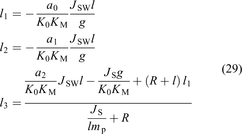
Then the equations describing the dynamics of the system without the influence of external forces are described

$\begin{array}{l}\left(m_{\text{w}}{R}^2+m_{\text{p}}{R}^2+J_{\text{w}}\right)\stackrel{\text{..}}{\varphi }+m_{\text{p}}lR\cos \left(\theta \right)\stackrel{\text{..}}{\theta }-m_{\text{p}}lR{\dot{\theta }}^2\text{sin}\left(\theta \right)=0\\ m_{\text{p}}lR\stackrel{\text{..}}{\varphi }\cos \left(\theta \right)+m_{\text{p}}{l}^2\stackrel{\text{..}}{\theta }+m_{\text{p}}gl\text{sin}\left(\theta \right)=0\end{array}$

13

Actuator is located in rotational linkage of AMAV. This actuator affects the wheels and body with torque M _P according to the rules of release in the opposite direction. Viscous friction M _DW counteracts against the movement of the wheels, damping with torque M _DP counteracts against the movement of pendulum, and viscous resistance with torque M _P is active in the rotational linkage (Figure 6). These torques are defined

$\begin{array}{l}{M}_{\text{DW}}=b_{\text{s}}\dot{\varphi }\\ M_{\text{F}}=b_{\text{F}}\left(\dot{\theta }-\dot{\varphi }\right)\\ M_{\text{DP}}=d_{\text{P}}\dot{\theta }\end{array}$

14

Where b _S is viscous damping coefficient of rolling of wheels, b _F is coefficient of viscous resistance in linkage wheel pendulum, and d _P is damping coefficient of body.

Figure 6.

Driving and damping torques acting on the AMAV. AMAV: ambiguous mono axial vehicle.

After integration of these equations in a dynamic description of the system

$\begin{array}{l}\left(m_{\text{w}}{R}^2+m_{\text{p}}{R}^2+J_{\text{w}}\right)\stackrel{\text{..}}{\varphi }+m_{\text{p}}lR\cos \left(\theta \right)\stackrel{\text{..}}{\theta }-m_{\text{p}}lR{\dot{\theta }}^2\text{sin}\left(\theta \right)\\ =-b_{\text{S}}\dot{\varphi }+b_{\text{F}}\left(\dot{\theta }-\dot{\varphi }\right)+M_{\text{p}}\\ m_{\text{p}}lR\stackrel{\text{..}}{\varphi }\cos \left(\theta \right)+m_{\text{p}}{l}^2\stackrel{\text{..}}{\theta }+m_{\text{p}}gl\text{sin}\left(\theta \right)=-b_{\text{F}}\left(\dot{\theta }-\dot{\varphi }\right)\\ -M_{\text{P}}-d_{\text{P}}\dot{\theta }\end{array}$

15

The value ${\dot{\theta }}^2$ is very close to zero. After this adjustment, equations describing the dynamics of AMAV (Figure 7)

$\begin{array}{l}\stackrel{\text{..}}{\varphi }=-\frac{b_{\text{S}}}{J_{\text{S}}}\dot{\varphi }-\frac{b_{\text{F}}}{J_{\text{S}}}\dot{\varphi }+\frac{b_{\text{F}}}{J_{\text{S}}}\dot{\theta }-\frac{m_{\text{p}}lR}{J_{\text{S}}}\cos \left(\theta \right)\stackrel{\text{..}}{\theta }+\frac{M_{\text{P}}}{J_{\text{S}}}\\ \stackrel{\text{..}}{\theta }=-\frac{b_{\text{F}}}{m_{\text{p}}{l}^2}\dot{\theta }-\frac{d_{\text{P}}}{m_{\text{p}}{l}^2}\dot{\theta }+\frac{b_{\text{F}}}{m_{\text{p}}{l}^2}\dot{\varphi }-\frac{R}{l}\cos \left(\theta \right)\stackrel{\text{..}}{\varphi }\\ -\frac{g}{l}\text{sin}\left(\theta \right)-\frac{M_{\text{p}}}{m_{\text{p}}{l}^2}\\ J_{\text{S}}=m_{\text{w}}{R}^2+m_{\text{p}}{R}^2+J_{\text{w}}\end{array}$

16

Figure 7.

Simulation model of AMAV in Matlab Simulink. AMAV: ambiguous mono axial vehicle.

Simulations

As it was mentioned above, AMAV in stabile mode is similar to dicycle model and in unstable mode when the payload is pushed out is similar to Segway. Despite the model of AMAV was derived for the stable mode, the change into unstable mode can be performed by setting of initial angle value to π radians. In reality, it means that the chassis is reversed by 180° and the CG is pushed out above the wheels axis. During the simulations, angular position is evaluated for both cases. The simulation model is illustrated in Figure 7. The input value Initial Phi for the stable case is equal to 0 radians, and, for the unstable case, it is equal to π radians. The parameters of models are derived from the real robotic AMAV chassis (Figure 8). The parameters of this chassis are defined in the Table 1.

Figure 8.

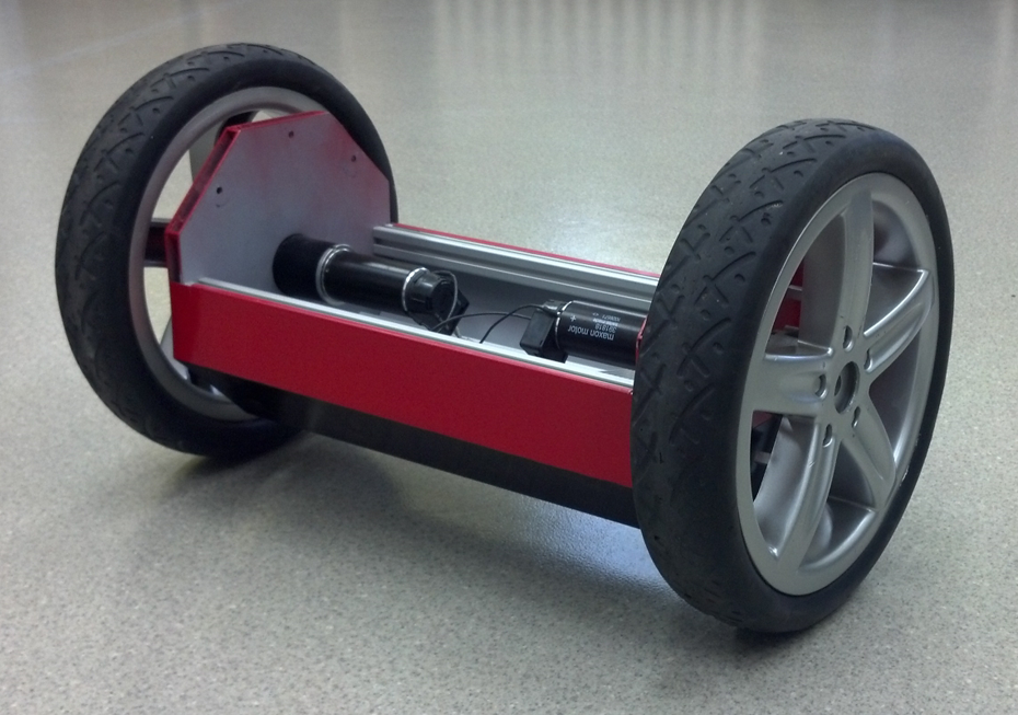
Real construction of mobile robotic chassis of AMAV type. AMAV: ambiguous mono axial vehicle.

Table 1.

The parameters of real AMAV.

Parameter	Value
m p (kg)	1.5
m w (kg)	1.4
L (m)	0.06
g (ms−2)	9.81
R (m)	0.1425
J W (kgm2)	0.0569
J S (kgm2)	0.1157
b F (Nms rad−1)	0.005
b S (Nms rad−1)	0.2
d P (Nms rad−1)	0.005

AMAV: ambiguous mono axial vehicle.

In the Figure 9, it can be seen AMAV response to input torque in a stable case (blue curve). The body of AMAV is unbalanced from the zero angular position (green curve) against the effecting input torque. Oscillating nature of the chassis can be seen during the transient effect in simulation time 1 s, 3 s, 5 s, and 7 s. Amplitude of these oscillations is not so high—maximum 0.01 radians. Body of AMAV has been shifted out of 0.225 radians against the zero position. Change of position during the influence of input torque was equal to 0.55 m (red curve).

Figure 9.

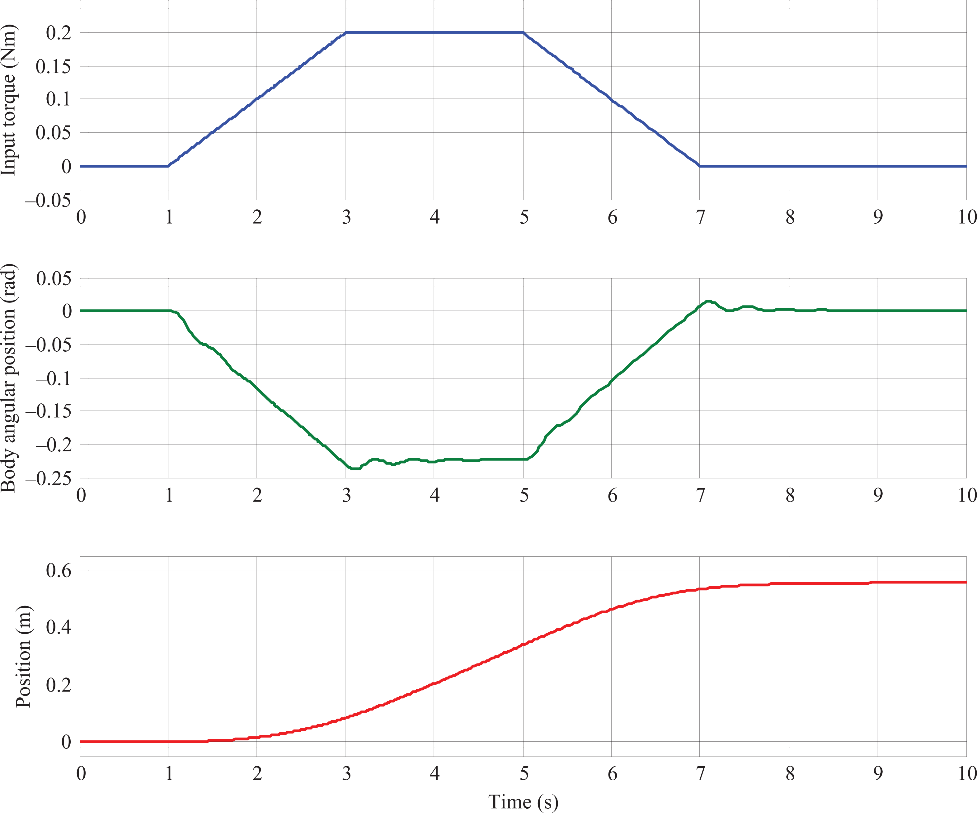
Simulation of dynamic model of AMAV at a stable mode. AMAV: ambiguous mono axial vehicle.

In the Figure 10, it can be seen AMAV response to input torque in an unstable case (blue curve). This means that the initial inclination (Initial Phi) was equal to π radians. From the results, it is clear that the body immediately begins swinging to stabilize its position. While the initial torque is constant, position of the body will stabilize at 0.2 radians. This is almost the same value as in the stable case. When the initial torque stops affecting AMAV, the body will stabilize on the angular position equal to 0 radians.

Figure 10.

Simulation of dynamic model of AMAV at an unstable mode. AMAV: ambiguous mono axial vehicle.

Proposed AMAV system is SIMO system, thus system with one input (torque generated by drive) and with two outputs (angular position of the body and angular position of the wheels). At this point, it is good to notice that only forward–backward motion is considered. This simplification will be taken into account for consequent analysis and control synthesis, because it is assumed that the essential mass constituting the body will be symmetrically distributed in it. The simulations show that non-controlled chassis is not able to hold the body position at the zero value during the application of input torque. In unstable mode, it is even worse that whole body is inverted. This may actually lead to the destruction of the chassis. Therefore, the control of AMAV is aimed to control the input torque (in fact the control of current in motors) on the basis of measured variables (angular positions and velocities of body and wheels) in such a way that the angular position of the body will change minimally from the zero value.

Generalized dynamic model of AMAV

The change from the stable case into the unstable case was realized by setting the initial position of body—either 0° or 180°. This setting is not suitable for the synthesis of united control for both modes (stable/unstable). That is why the generalized dynamic model of AMAV will be derived on the basis of generalized position of CG. The position of the CG is conceptualized as the pendulum length defined by mathematical model of AMAV (Figure 5). If the damping elements are neglected, then the AMAV model is described

$\begin{array}{l}{J}_{\text{S}}\stackrel{\text{..}}{\varphi }+m_{\text{p}}lR\stackrel{\text{..}}{\theta }\cos \left(\theta \right)-m_{\text{p}}lR{\dot{\theta }}^2\text{sin}\left(\theta \right)=M_{\text{p}}\\ m_{\text{p}}lR\stackrel{\text{..}}{\varphi }\cos \left(\theta \right)+m_{\text{p}}{l}^2\stackrel{\text{..}}{\theta }+m_{\text{p}}gl\text{sin}\left(\theta \right)=-M_{\text{P}}\end{array}$

17

The change from the unstable state into the stable one was realized by adding 180° to angular position

$\begin{array}{l}\text{sin}\left(\theta +180\right)=-\text{sin}\left(\theta \right)\\ \cos \left(\theta +180\right)=-\cos \left(\theta \right)\end{array}$

18

At the same time, the model will change consequently

$\begin{array}{l}{J}_{\text{S}}\stackrel{\text{..}}{\varphi }-m_{\text{p}}lR\stackrel{\text{..}}{\theta }\cos \left(\theta \right)+m_{\text{p}}lR{\dot{\theta }}^2\text{sin}\left(\theta \right)=M_{\text{p}}\\ -m_{\text{p}}lR\stackrel{\text{..}}{\varphi }\cos \left(\theta \right)+m_{\text{p}}{l}^2\stackrel{\text{..}}{\theta }-m_{\text{p}}gl\text{sin}\left(\theta \right)=-M_{\text{P}}\end{array}$

19

Each member of the equation, which changed the sign, also contains the pendulum length l. That is why the generalized position of CG can be introduced into a dynamic model of the system and it will change consequently:

If the CG is under the wheels axis, l > 0.

If the CG is in the wheels axis, l = 0.

If the CG is above the wheels axis, l < 0.

By this definition, the angle θ does not change when the mode is changed from stable to unstable and vice versa. Accordingly only the sign of the generalized position of CG is changed. This is very useful in consequent analysis and synthesis of control.

It is appropriate to linearize the differential equations of generalized dynamic model of AMAV for the synthesis of control. In this case, the viscous damping of rolling wheels, viscous resistance in linkage wheel-pendulum and damping of body is neglected. This assumption can be applied because if the generalized position of the CG l is positive, AMAV is in stable mode and the aim of control is to damp the oscillations of AMAV body. In such control, damping will rather aid and it will not change the sense of linkages. In like manner when the generalized position of the CG is negative and system is in unstable mode, damping will counteract against the body’s motion and this will rather aid in stabilization of the body’s position around 0°. Linearization will be done in the surrounding θ = 0 and $\dot{\theta }=0$ :

$\begin{array}{l}\text{sin}\theta =\theta \\ \cos \theta =1\\ J_{\text{S}}\stackrel{\text{..}}{\varphi }+m_{\text{p}}lR\stackrel{\text{..}}{\theta }=M_{\text{p}}\\ m_{\text{p}}lR\stackrel{\text{..}}{\varphi }+m_{\text{p}}{l}^2\stackrel{\text{..}}{\theta }+m_{\text{p}}gl\theta =-M_{\text{P}}\end{array}$

20

And then linearized equations are defined

$\begin{array}{l}\stackrel{\text{..}}{\varphi }=\frac{M_{\text{p}}}{J_{\text{S}}}-\frac{m_{\text{p}}lR}{J_{\text{S}}}\stackrel{\text{..}}{\theta }\\ \stackrel{\text{..}}{\theta }=-\frac{M_{\text{p}}}{m_{\text{p}}{l}^2}-\frac{R}{l}\stackrel{\text{..}}{\varphi }-\frac{g}{l}\theta \end{array}$

21

Transfer function is then described

$\frac{\varphi \left(s\right)}{M_P\left(s\right)}=\frac{\frac{l+R}{g}{s}^2+1}{\frac{m_W{R}^2+J_W}{g}l{s}^4+J_S{s}^2}$

22

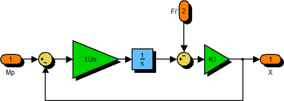
The simulation scheme to the corresponding linearized model is shown in Figure 11.

Figure 11.

Scheme of the linearized dynamic model of AMAV. AMAV: ambiguous mono axial vehicle.

In the case that l = +0.06 m, system is in stable mode. The poles and zeros of system can be seen in Figure 12. In this mode system has four poles, two are placed in zero and two appear in complex conjugate pair: 0 + 18.24i and 0 − 18.24i. It is clear that the damping is neglected and, therefore, the system is on the margin of stability.

Figure 12.

Poles and zeros of system in stable mode.

In the case that l = −0.06 m, system is in unstable mode. The poles and zeros of system can be seen in Figure 13. In this mode system has four poles, two are placed in zero, one is stable at −18.24 + 0i, and one is unstable at 18.24 + 0i. These characteristics will be used in synthesis of control for both modes.

Figure 13.

Poles and zeros of system in unstable mode.

Synthesis of control

As it was mentioned earlier, proposed AMAV system is SIMO system with one input (torque generated by drive) and with two outputs (angular position of the body and angular position of the wheels). These two outputs correspond to relevant and practically measureable state variables, which are defined in Table 2.

Table 2.

State variables of AMAV system.

State variable	Description
ϕ(s)	Angular position of the wheels
$\dot{\varphi }\left(s\right)$	Angular velocity of the wheels
θ(s)	Angular position of the body
$\dot{\theta }\left(s\right)$	Angular velocity of the body

AMAV: ambiguous mono axial vehicle.

Controlled variable is the torque generated by drive, which is defined in the linkage between the body and the wheel. Naturally in real AMAV, the generator of this torque is electric motor. In proposed AMAV system, MAXON DC motor ¹⁷ with planetary gear controlled by converter under current-mode control is used. The original model did not taken into account this drive. Therefore, it will be added to the control structure as simplified system of first order with total gain K _M and total time constant T _M, which define the dynamic properties of the drive

$G_{\text{P}}\left(s\right)=\frac{K_{\text{M}}}{T_{\text{M}}s+1}$

23

The main requirements on the control are damping of body’s oscillations in stabile mode and stabilization of AMAV in unstable mode. That is why the state-space control with pole placement will be used. ¹⁸ Scheme for the state-space control is illustrated in Figure 14.

Figure 14.

Scheme of state-space control for AMAV. AMAV: ambiguous mono axial vehicle.

Gains K _M, K ₀, and time constant T _M are the values, which can be obtained from MAXON catalogue. ¹⁷ Time constants of AMAV (as it was shown earlier) are in units of seconds and time constant T _M is in hundredths of seconds. That is why this time constant will be neglected in following synthesis. Then the transfer function is defined:

$\frac{\varphi \left(s\right)}{w_{\text{P}}\left(s\right)}=\frac{K_0{K}_{\text{M}}\left(\frac{l+R}{g}{s}^2+1\right)}{\begin{array}{l}{s}^4\frac{m_{\text{W}}{R}^2+J_{\text{W}}}{g}l+s^3\frac{K_0{K}_{\text{M}}}{g}\left(\left(\frac{J_{\text{S}}}{gl{m}_{\text{p}}}+R\right)l_4-\left(R+l\right)l_2\right)\\ +s^2\frac{K_0{K}_{\text{M}}}{g}\left(\frac{J_{\text{S}}g}{K_0{K}_{\text{M}}}+\left(\frac{J_{\text{S}}}{l{m}_{\text{P}}}+R\right)l_3-\left(R+l\right)l_1\right)+s\left(-K_0{K}_{\text{M}}{l}_2\right)\\ +\left(-K_0{K}_{\text{M}}{l}_1\right)\end{array}}$

24

From the transfer function it is clear that the system will stabilize at a value −1/l ₁. However, it is not desirable. Hence, the gain compensation will be introduced into the control scheme. Characteristic polynomial of the system is defined

$\begin{array}{l}A\left(s\right)=s^4\frac{m_{\text{W}}{R}^2+J_{\text{W}}}{g}l\\ +s^3\frac{K_0{K}_{\text{M}}}{g}\left(\left(\frac{J_{\text{S}}}{gl{m}_{\text{p}}}+R\right)l_4-\left(R+l\right)l_2\right)\\ +s^2\frac{K_0{K}_{\text{M}}}{g}\left(\frac{J_{\text{S}}g}{K_0{K}_{\text{M}}}+\left(\frac{J_{\text{S}}}{L{m}_{\text{P}}}+R\right)l_3-\left(R+L\right)l_1\right)\\ +s\left(-K_0{K}_{\text{M}}{l}_2\right)+\left(-K_0{K}_{\text{M}}{l}_1\right)\end{array}$

25

Let the system of fourth order is divided into two subsystems of second order. First subsystem will describe the properties of AMAV body and second subsystem will describe the properties of drive. Desired characteristic polynomial is defined

$\begin{array}{l}{A}_{\text{D}}\left(s\right)=\left(s^2+2b_1{\omega }_{01}s+{\omega }_{01}^2\right)\left(s^2+2b_2{\omega }_{02}s+{\omega }_{02}^2\right)\\ =s^4+s^{3}2\left(b_1{\omega }_{01}+b_2{\omega }_{02}\right)+s^2\left({\omega }_{01}^2+{\omega }_{02}^2\right)\\ +s2\left(b_1{\omega }_{01}^2{\omega }_{02}+b_2{\omega }_{02}^2{\omega }_{01}\right)+{\omega }_{01}^2{\omega }_{02}^2\\ a_3=2\left(b_1{\omega }_{01}+b_2{\omega }_{02}\right)\\ a_2={\omega }_{01}^2+{\omega }_{02}^2\\ a_3=b_1{\omega }_{01}^2{\omega }_{02}+b_2{\omega }_{02}^2{\omega }_{01}\\ a_0={\omega }_{01}^2{\omega }_{02}^2\\ A_{\text{D}}\left(s\right)=s^4+a_3{s}^3+a_2{s}^2+a_{1}s+a_0\end{array}$

26

Synthesis of controller by the pole placement methods allows placement the poles of system on the basis of desired dynamical characteristics of the system. If desired characteristic polynomial is equal to characteristic polynomial

$\begin{array}{l}{a}_3=\frac{K_0{K}_{\text{M}}}{J_{\text{SW}}l}\left(\left(\frac{J_{\text{S}}}{gl{m}_{\text{p}}}+R\right)l_4-\left(R+l\right)l_2\right)\\ a_2=\frac{K_0{K}_{\text{M}}}{J_{\text{SW}}l}\left(\frac{J_{\text{S}}g}{K_0{K}_{\text{M}}}+\left(\frac{J_{\text{S}}}{l{m}_{\text{P}}}+R\right)l_3-\left(R+l\right)l_1\right)\\ a_1=\frac{g}{J_{\text{SW}}l}\left(-K_0{K}_{\text{M}}{l}_2\right)\\ a_0=\frac{g}{J_{\text{SW}}l}\left(-K_0{K}_{\text{M}}{l}_1\right)\end{array}$

27

Where

$J_{\text{SW}}=m_{\text{w}}{R}^2+J_{\text{W}}$

28

The gains of the controller are then defined as follows

$\begin{array}{l}{l}_1=-\frac{a_0}{K_0{K}_{\text{M}}}\frac{J_{\text{SW}}l}{g}\\ l_2=-\frac{a_1}{K_0{K}_{\text{M}}}\frac{J_{\text{SW}}l}{g}\\ l_3=\frac{\frac{a_2}{K_0{K}_{\text{M}}}{J}_{\text{SW}}l-\frac{J_{\text{S}}g}{K_0{K}_{\text{M}}}+\left(R+l\right)l_1}{\frac{J_{\text{S}}}{l{m}_{\text{p}}}+R}\end{array}$

29

$l_4=\frac{\frac{a_3}{K_0{K}_{\text{M}}}{J}_{\text{SW}}l+\left(R+l\right)l_2}{\frac{J_{\text{S}}}{l{m}_{\text{p}}}+R}$

30

From the characteristic polynomial, it is clear that there are two pole couples. It is needed to suitably arrange these couples in complex plane. First pole couple is slow and second couple is fast (Figures 12 and 13). Fast pole couple is represented by AMAV body (replaced by inverted pendulum) and slow pole couple is represented by overall dynamics of AMAV. This is the basic assumption when the damping parameters b ₁ and b ₂ and natural angular frequencies ω ₀₁ and ω ₀₂ will be determined. ¹⁹ Based on the empirical experience, damping coefficients are selected from the interval 0.5–0.707. In the case of pole placement controller, the values b ₁ = b ₂ = 1/√2 = 0.707 were selected for both pole couples. On the basis of motor parameters, maximal angular acceleration is specified:

${\dot{\omega }}_{\text{MAX}}=\frac{I_{\text{MAX}}{K}_{\text{M}}}{J_{\text{S}}}=\frac{4\times 0.2328}{0.1157}=8.0484\text{\hspace{0.17em}rad}.{\text{s}}^{-2}$

31

The value ω₀₁ is specified as $1/2{\dot{\omega }}_{\text{MAX}}$ . In next step, the controller gains l ₁, l ₂, l ₃, and l ₄ are determined on the basis of change in ω₀₂ specified in the interval 〈0.5ω_02O,2ω_02O〉. The parameter ω ₀₂ is natural angular frequency of the system equal to 18.24 (as it can be seen in Figure 12). The controller gains change in proportion to ω₀₂/ω_02O—with increasing ω ₀₂ controller gains increase exponentially (Figure 15). However, the controller gains should be as small as possible, because if the gains will be greater, then the input to the system will be greater too. Accordingly, motors are limited by some physical constraints, that is, current and coupled torque limit. Moreover, it is useful to hold the system around the natural frequency. Based on these facts ω₀₂ is selected as 1.5 × ω _02O. At this value, the gain l₄ is very close to zero, and gains l₁, l₂, and l₃ are around the value 1. It follows that the value ω ₀₂ = 27.36 rad.s⁻¹. This pole placement will be verified as linearized system, as well as nonlinear system with damping, in both stable and unstable mode.

Figure 15.

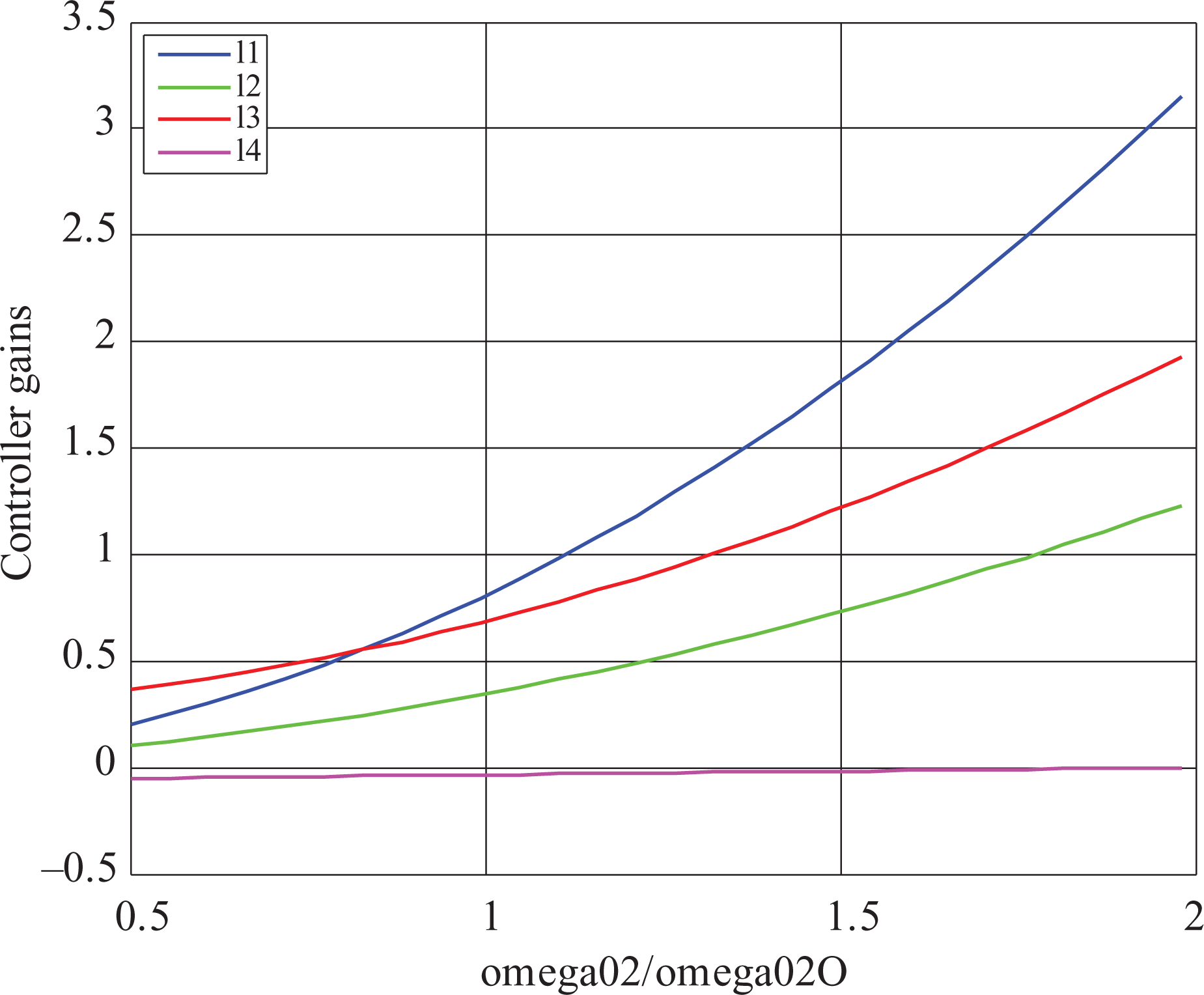
Dependency of controller gains on the desired natural angular frequency of the system (ω ₀₂).

As it was mentioned earlier, it is necessary to introduce the compensation of gain l ₁. The final scheme of the control is shown in Figure 16.

Figure 16.

Resultant scheme of control.

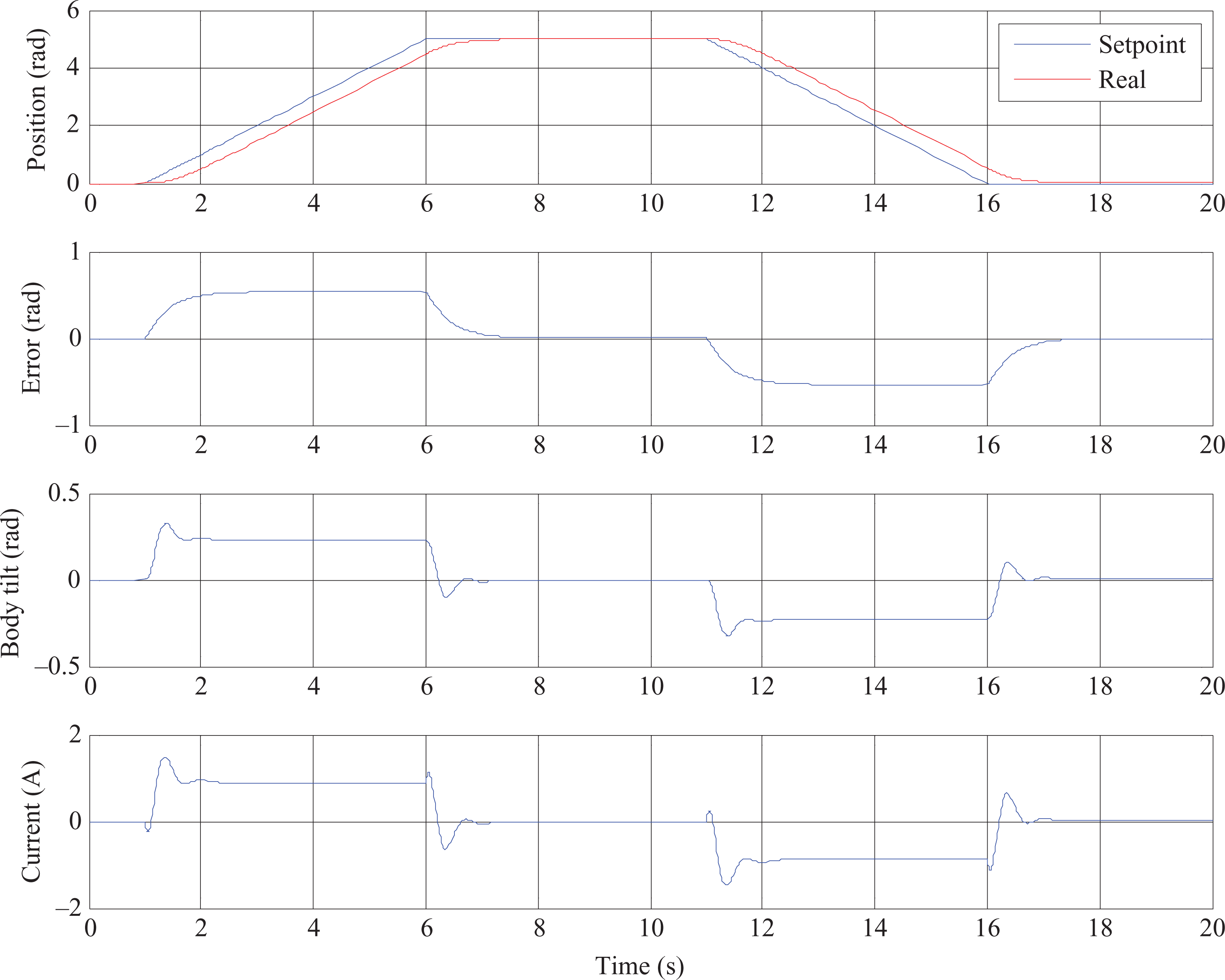
The desired value of the position is characterized as trapezoidal signal from the trajectory generator, whereby the reaction of AMAV on that signal is observed. Observed variables are real position of the wheels, inclination of AMAV and consumed current.

The simulation for the linearized model in stable mode is shown in Figure 17. It can be seen that the position error during the slope and run down of desired position is equal to 0.4 rad. The AMAV body is deviated from the vertical position of about 0.3 rad and always against the opposite side of performed motion. Likewise, the current increases to around 1 A. During the steady motion, the current consumption is equal to 0, because the linearized system does not have any damping. It is clear that the motion of AMAV body has aperiodic character due to foisted damping. AMAV is also capable enough to follow the desired position. It is suitable to verify the pole placement of closed control loop in the dependency on degree of systems constrains. This means that the controller gains will change in the interval 〈0, {l₁, l₂, l₃, l₄}〉. This dependency (a geometric viewpoint) is shown in Figure 18. At the beginning, the original pole couple will slightly accelerate and the damping will increase to desired value 0.707. This couple will stabilize on the values −2.845 − 2.845i and −2.845 + 2.845i. Fast pole couple will tear away from imaginary axis to the left due to increased damping equal to 0.707 and due to increased natural frequency, which is equal to 27.36 rad.s⁻¹. Its position will stabilize at −19.35 + 19.35i and −19.35 − 19.35i.

Figure 17.

Linearized model in stable mode.

Figure 18.

Dependency of pole placement on degree of systems constrains—linearized model, stable mode.

The simulation for the linearized model in unstable mode is shown in Figure 19. The position error remained unchanged in comparison with the stable mode. However, the body of AMAV is deviated from the vertical position in the opposite direction as in the stable case. This is required in unstable mode, because the generated torque must keep the upright position of the AMAV. In the case, the body of AMAV is inclined in the opposite direction, with increased generated torque the body of AMAV would tend to fall (positive feedback). Moreover, from the current course it can be seen that the controller respond only with small input to the system in opposite direction during the small change in motion—body is deviated in the direction of the motion. Consequently, input to the system in opposite direction is generated, which performs the actual motion and control of body’s position. The dependency of pole placement on degree of systems constrains is shown in Figure 20. It is clear that with increasing degree of systems constrains the pole couples will move against each other. This will reduce the couples into the single pole, in the left half-plane −6 + 0i and in the right half-plane 7 + 0i. From this torque, the poles are divided, whereby they move from the real axis little by little up to a predefined position −2.845 − 2.845i, −2.845 + 2.845i, −19.35 + 19.35i, and −19.35 − 19.35i. It is the same pole placement as in the stable mode.

Figure 19.

Linearized model in unstable mode.

Figure 20.

Dependency of pole placement on degree of systems constrains—linearized model, unstable mode.

In the verification of nonlinear model, the same control scheme was used. Linearized model was replaced by nonlinear of course. The simulation for the nonlinear model in stable mode is shown in Figure 21. It can be seen that the system behaves similarly as linearized model, only inclination of body and current do not stabilize at zero. This is due to damping, which was not taken into account within the linearized model. The consumed current is stabilized around 1 A, and the inclination of the AMAV body is stabilized around 0.25 rad.

Figure 21.

Nonlinear model in stable mode.

The simulation for the nonlinear model in unstable mode is shown in Figure 22. The difference between the nonlinear model and linear model in this mode is characterized as in the previous case. The consumed current is stabilized around 1 A, and the inclination of the AMAV body is stabilized around 0.25 rad. It can be also seen slight overshoot of current into opposite direction, which causes the deflection of AMAV body into the direction of the motion.

Figure 22.

Nonlinear model in unstable mode.

The gains of controller are derived on the basis of the constant length of inverted pendulum (hangings), which simulates the AMAV. When this length will change, the controller will not be able to guarantee the required characteristics of control. That is why it is suitable to associate the change of gains with the change of hangings length. As it was mentioned earlier, the payload of AMAV is pushed out only when the AMAV is not in forward/backward motion. The lookup table was created to determine the dependency of controller gains on hangings length. This was identified off-line in various lengths. An estimate of the current length of inverted pendulum is defined (Figure 11)

$\widehat{l}=\frac{K_{\text{M}}I-J_{\text{s}}\stackrel{\text{..}}{\varphi }}{R{m}_{\text{P}}\stackrel{\text{..}}{\theta }}$

32

This estimate has one serious disadvantage. Measurement of wheels angular acceleration $\stackrel{\text{..}}{\varphi }$ is very hard to realize in the real system. This can be realized by IRC sensor, but the second derivation of angular position, which is the output of IRC sensor, will introduce too high error in this measurement. Let’s look at the part of the dynamic model of AMAV in the Figure 23. There can be seen the influence of reactive torque between the body and wheels. The input to the summation is input torque M _P, from which the reactive torque proportional to length l is subtracted. From this, it can be derived

$\begin{array}{l}{M}_{\text{X}}=M_{\text{P}}-M_{\text{REAC}}\\ M_{\text{REAC}}=m_{\text{P}}R\widehat{l}\stackrel{\text{..}}{\theta }\\ M_{\text{x}}=J_{\text{S}}\stackrel{\text{..}}{\varphi }\end{array}$

33

Figure 23.

The part of the control scheme with highlighted influence of reactive torque between the body and wheels.

Introduction of observer (Figure 24) helps to suppress the problem of angular acceleration measuring. It follows

$\begin{array}{l}X=\frac{M_{\text{REAC}}}{\frac{J_{\text{S}}}{K_1}s+1}\\ \widehat{l}=\frac{X}{R{m}_{\text{P}}\stackrel{\text{..}}{\theta }}\end{array}$

34

Figure 24.

The scheme of reactive torque observer.

It is thus possible to measure the length of hangings without the need for measurement of wheels angular acceleration. Angular acceleration of the body can be measured by gyro, which output is angular velocity of the body.

Conclusions and future work

Concept of AMAV mobile robot was introduced in this article. The key characteristic of such robot is the change of CoG’s position within the body of AMAV. This leads to the change of system’s characteristics from stable oscillating into unstable, and vice versa. Generalized mathematical model of such system was also derived. This model is based on generalized distance of CoG from the axis of wheels and it was used to propose the control by pole-placement method. This control was verified by simulations for linear and nonlinear (in operating points) model and also for stable and unstable regime. Based on the simulations analysis, estimation of parameter L (generalized distance of CoG from the axis of wheels) was also derived. Moreover, the rules for adaptation of system’s control to this parameter were also proposed. For the future work, we are working on implementation of whole control scheme into the real AMAV. We would like to exactly verify the generalized model and proposed control on real AMAV.