
Abstract
In this article, a constraint factor is introduced into the hysteretic operator so that the hysteretic operator can pass through the origin in every minor coordinate system. Based on the hysteretic operator, an expanded input space is constructed. And then, it is proved that the mapping between the expanded input space and the output space contains only one-to-one mapping and multiple-to-one mapping, which can be identified using the traditional methods of neural networks. Finally, a neural network is employed to model hysteresis for the magnetostrictive sensors and actuators. Two experiments are implemented to validate the neural hysteresis model. The experimental results demonstrate that the proposed approach is effective.
Keywords
Introduction
Based on the magnetostrictive effect, magnetostrictive materials are usually used for sensors and actuators. 1 Because of their excellent characteristics, such as large output force, high position resolution, fast response speed, and low creep, magnetostrictive sensors and actuators have been widely applied to ultrahigh precision positioning systems, 2 electric vehicle, 3 vehicle safety system, 4 air vehicle, 5 and so on. However, a nonlinear phenomenon, hysteresis, which is nonsmooth, nondifferentiable, nonmemoryless, and multivalued mapping, exists in magnetostrictive sensors and actuators. For control systems, hysteresis can frequently lead to inaccuracy, stick–slip motions, undesired oscillations, and even instability. 6 To compensate the negative effects of hysteresis, model-based control strategies are usually adopted in control systems. 7 Therefore, it is important for magnetostrictive sensors and actuators to construct accurate hysteresis models. A large number of hysteresis models have been proposed in the past decades. Among these hysteresis models, the operator-based hysteresis models, such as Prandtl–Ishlinskii (PI) model, 8 Preisach model, 9 and Krasnosel’skii-Pokrovskii model, 10 were the most frequently used in control systems. However, with the development of science and technology, the control systems are increasingly requiring more accurate hysteresis models.
Neural networks (NNs) have been viewed as one of the best methods of modeling hysteresis. But it has been proved that the NNs cannot be directly used to identify the multivalued mapping of hysteresis. 11 The multivalued mapping consists of one-to-multiple and multiple-to-one mappings, while the NNs can only identify one-to-one mapping and multiple-to-one mapping. Therefore, the one-to-multiple mapping has to be eliminated in order to construct neural hysteresis model. Ma 12 presented a hysteretic operator (HO) and established a two-dimension input space based on the HO. In the expanded input and output spaces, the one-to-multiple mapping can be transformed into a one-to-one mapping so that a neural hysteresis model can be constructed. Since then, several neural hysteresis models have been proposed. 13 –17
In this article, a constraint factor is introduced into the HO containing a constant term, so that the HO can pass through the origin point. And then, it is proved that the one-to-multiple mapping of hysteresis can be transformed into one-to-one mapping based on the constructed HO. Finally, a neural hysteresis model was developed and used for approximation of a set of real data from a magnetostrictive actuator. The approximation performance approved the proposed approach.
Construction of HO
Definition of HO
In this article, an odd m-order polynomial with the constant term is used as the HO. However, the curve of the HO should pass through the origin point in every minor coordinate system, so a constraint factor,

where xi is any input and f is the corresponding output of HO in the ith minor coordinate system.
In the main coordinate system, the HO is expressed as
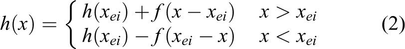
where [xei , h(xei )] are the origin coordinates of the ith minor coordinate system, x is any input, and h is the corresponding output of HO in the main coordinate system.
Model structure
In this article, the output of the HO and the input of hysteresis are together fed into NNs so that the input space is expanded from one dimension to two dimension (shown as Figure 1). The NN equation can be written as

Model structure.

where W T = [wj ]T and V T = [vij ]T are the weight matrices, i = 1, 2; j = 1, 2, …, N; X = [x(t), h(t)]T. The scalar function σ(·) is a sigmoidal activation function of the hidden layer neurons.
Model parameters
As well known to all, the least square method is the best method of determining the polynomial parameters. Thus, the n samples used for NN training is used to calculate the model parameters.
In terms of the least square method, the residual δi is

So the sum of square residuals is as follows

To minimize the sum S, the partial derivatives of S with regard to a 0, a 1, … , am are set as zero, and equation (6) is given

Rearranging equation (6) gives
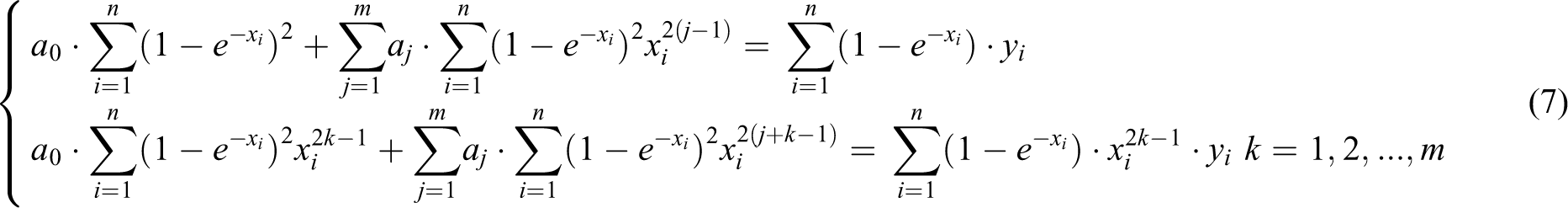
Expanding equation (7) as follows

The equivalent matrix equation of equation (8) is


Solving equation (10) gives the parameters expression

Only if X is full rank matrix, equation (10) has a unique solution. In the following, it will be proved that the matrix X has full rank, that is, rank (X) = (m + 1), assuming that (m + 1) is smaller than or equal to n.
Proof: let

Because x 1 ≠ x 2 ≠ … ≠ xn , the (m + 1) columns of the matrix M are linearly independent, that is, the matrix M is column full rank. And since (m + 1) ≤ n, rank = (m + 1).
And since the row rank of the transpose matrix MT equals the column rank of the matrix M, so the MT is a row full rank matrix, that is, rank (MT ) = (m + 1).
The matrix X can be written as

Therefore, rank (X) = min [rank (M), rank (MT )]. And since rank (M) = rank (MT ) = (m + 1), rank (X) = (m + 1). Therefore, the matrix X is full rank.
In conclusion, assuming that the parameter number of the polynomial (m + 1) is smaller or equal to the sample number, n, equation (10) has a unique solution.
Mapping between the input and output spaces
The multivalue mapping of hysteresis includes one-to-multiple and multiple-to-one mappings, while the one-to-multiple mapping cannot be identified using the traditional approach of NNs. As shown in Figure 2, for the times t 1 and t 2, the corresponding inputs x(t 1) and x(t 2) are equal, while the outputs y(t 1) and y(t 2) are unequal. That is to say, the two equal inputs are corresponding to the two different outputs, which is the so-called one-to-multiple mapping. In this article, the input space is expanded from one dimension to two dimension by adding the output h[x(t)] of HO into the input space. In this way, it is decisive that whether or not the one-to-multiple mapping can be transformed into a one-to-one mapping in the expanded spaces. If the one-to-multiple mapping can be transformed into a one-to-one mapping, the approach is successful and vice versa.

Multivalue mapping of hysteresis.

Analogously, the h(x e2) is

In the minor coordinate system with origin [xe 2, h(x e2)], since x > xe 2, according to equation (2), the h[x(t 2)] is

And because x 2 = x 1

Substituting the equation (15) into the equation (16) gives

Subtracting the equation (17) from the equation (14) gives

Let
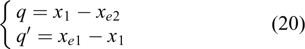
Then

Substituting the equations (20) and (21) into equation (18) gives

In every minor coordinate system, the branch of hysteresis loop is similar to an S-curve which passes through the origin. Since the curve f(x) is fitted by the least square method, it is similar to an S-curve as shown in Figure 3. If there exist three intersection points at least between the f(x) and f
1(x) besides the origin, then

The curves of f(x) and f 1(x).
Thus, for two different times t 1 and t 2, even though x(t 1) = x(t 2), it can lead to h[x(t 1)] ≠ h[x(t 2)].

Then

It is clear that h[x(t 2)] − h[x(t 1)] → 0 leads to x(t 2) − x(t 1) → 0.
Between the expanded input and output spaces, for the times t 1 and t 2, according to Lemma 1

And because y(t 1) and y(t 2) are unequal, (x(t 1), h[x(t 1)]) → y(t 1) and (x(t 2), h[x(t 2)]) → y(t 2) are two different mappings. Therefore, the one-to-multiple mapping is transformed into a one-to-one mapping.
In the following, the one-to-one mapping will be proved continuous.
In accordance with ref. 18

Then, in terms of Lemma 2

So the mapping is continuous.
Therefore, for any hysteresis nonlinearity, it can be concluded that the one-to-multiple mapping can be transformed into a continuous one-to-one mapping by expanding the input space from one dimension to two dimension based on the proposed HO.
As is well known, any continuous one-to-one or multiple-to-one mapping can be identified to arbitrary accuracy on a compact set using a three-layer NN that contains a sufficient quantity of hidden nodes. 19
Experimental validation
In this section, the proposed model is compared with the PI model and the model in ref. 17 so as to verify the effectiveness of the proposed approach. In the two experiments, the proposed model and the PI model were used to approximate a set of real data from a magnetostrictive actuator.
The experimental platform was made up of a magnetostrictive actuator (MFR OTY77), a current source, a personal computer, and a dSPACE control board with a 16-bit analog-to-digital and digital-to-analog converters. Under the excitation of a current at frequency up to 1.25 kHz, the actuator has a peak-to-peak output displacement of 100 μm. A set of data containing 1916 input–output pairs is acquired and separated into two groups equally. One group is used for NNs training, and another group for model validation.
The proposed model
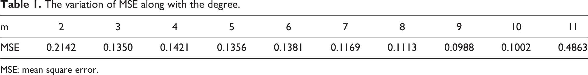
In this section, the neural hysteresis model involving a three-layer feed-forward NN is employed to approximate the real data. The activation functions of the hidden and output layers are, respectively, sigmoid and linear functions. Table 1 lists the mean square errors (MSEs) of the neural hysteresis model with different HO degrees. It can be seen from Table 1 that the model with degree 9 has the best result. Thus, m = 9.
The variation of MSE along with the degree.
MSE: mean square error.
To determine the optimal number of hidden nodes, the number from 1 to 100 is tried in the experiment. Taking into account the limited paper length, only the top 3 performances are listed in the Table 2. Table 2 shows that the neural model with 5 hidden nodes has the smallest MSE. Therefore, an NN consisting of two input nodes, five hidden nodes, and one output node is employed to approximate the real data from the magnetostrictive actuator. After 351 iterations, the training procedure is finished. Figures 4 and 5 show the validation result and absolute errors, respectively. The MSE, maximum absolute error, mean relative error, maximum relative error, and calculation time are shown in Table 3.
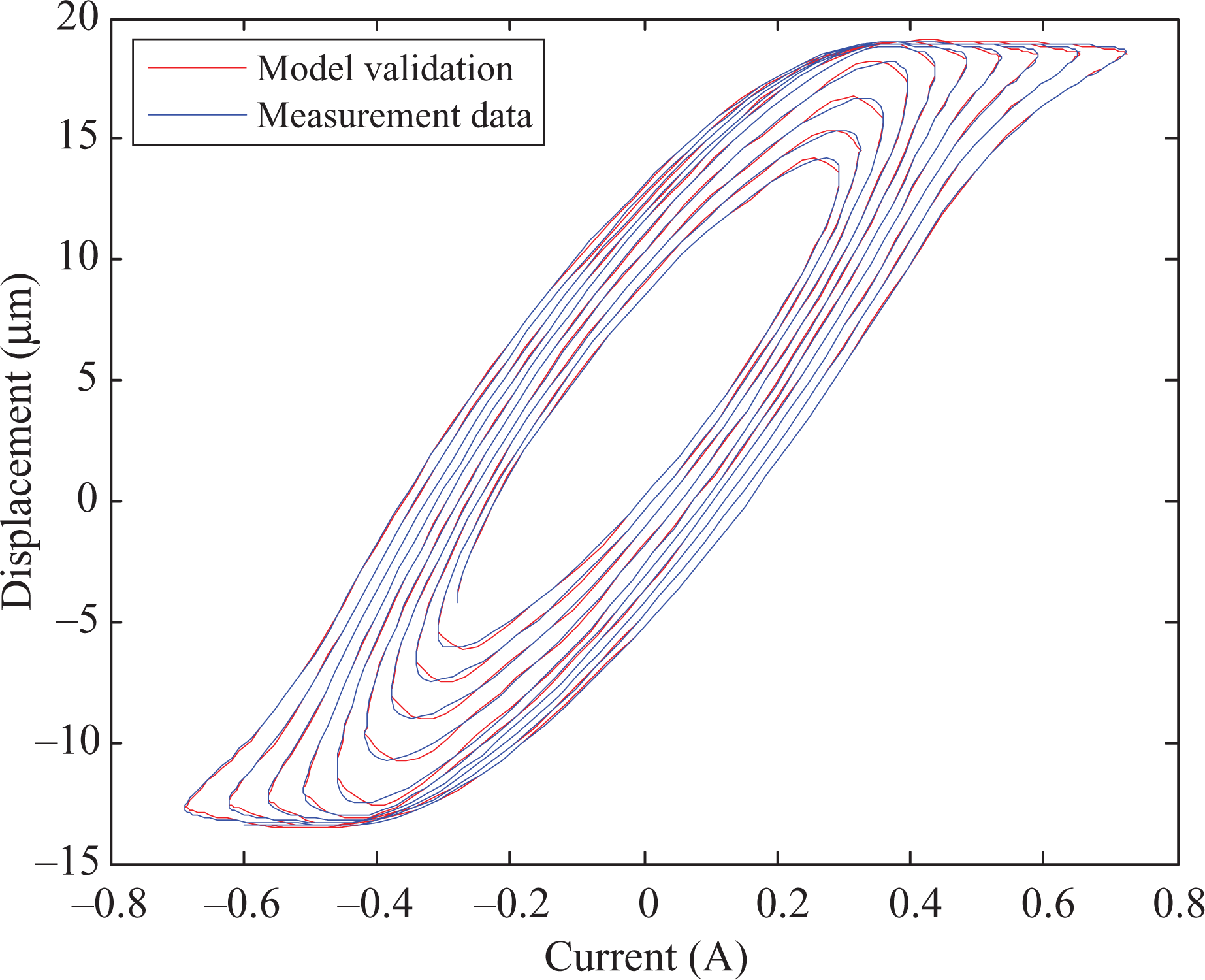
Comparison of the proposed model prediction and the real data.

The absolute error of the proposed model.
The top three performances of NN with different number of hidden neurons.

MSE: mean square error; NN: neural network.
Comparison of the proposed model with the other models.
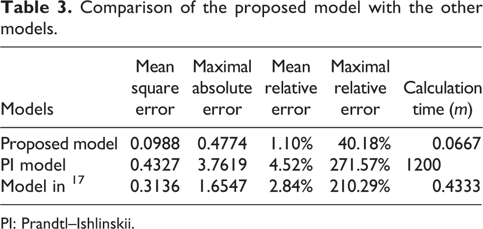
PI: Prandtl–Ishlinskii.
The PI model
Besides, the PI model was compared with the proposed model by approximating the real data. The operator thresholds were calculated in accordance with the following formula

where N is the number of backlash operators, and i = 1, 2, …, N.
The weights were determined by using the Matlab nonlinear optimization function. The MSE decreases along with the increase of N, while the computation time increases. Thus, N from 1 to 5000 is tried. It was found that N = 4994 has the best approximation result, which leads to a 20-hour calculation time. Figures 6 and 7 show the validation result and absolute errors, respectively. The MSE, maximum absolute error, mean relative error, maximum relative error, and calculation time are shown in Table 3.

Comparison of the Prandtl–Ishlinskii (PI) model prediction and the real data.

The absolute error of the Prandtl–Ishlinskii (PI) model.
The model in ref. 17
To compare with the proposed model, the model presented in ref. 17 was also adopted to approximate the set of real data from the magnetostrictive actuator. An NN containing 2 input nodes, 90 hidden nodes and 1 output node was employed. After 1064 iterations, the training procedure was finished. Figures 8 and 9 show the validation result and absolute errors, respectively. The MSE, maximum absolute error, mean relative error, maximum relative error, and calculation time are shown in Table 3.

Comparison of the prediction of the model in ref. 17 and the real data.

The absolute error of the model in ref. 17
Comparison
It can be viewed from the Table 3, in comparison with the PI model and the model in ref. 17 with regard to the MSE, maximal absolute error, mean relative error, maximal relative error, and calculation time, the proposed model can better approximate the measured data from the magnetostrictive actuator.
Conclusions
In this article, a new HO containing a constraint factor and an odd m-order polynomial is proposed. And then, the one-to-multiple mapping of hysteresis is transformed into a continuous one-to-one mapping based on the HO. It is well known that one-to-one mapping can be identified using NNs. Finally, a neural hysteresis model is constructed and two experiments are implemented to validate it. The experimental results suggest that the proposed approach is effective.
Footnotes
Declaration of conflicting interests
The author(s) declared no potential conflicts of interest with respect to the research, authorship, and/or publication of this article.
Funding
The author(s) disclosed receipt of the following financial support for the research, authorship, and/or publication of this article: This work was supported in part by National Natural Science Foundation of China (Grant nos. 11304282 and 61540034); the Zhejiang Open Foundation of the Most Important Subjects; Zhejiang Provincial Natural Science Foundation (Grant nos. LQ14F050002, LQ15F030008, LQ16F030002, and LY16F030007); Science Technology Department of Zhejiang Province (Grant no. 2014C31020); and Qiuxuan wu was also supported by a grant from the China Scholarship Council.