
Abstract
In this article, an adaptive neural dynamic surface sliding mode control scheme is proposed for uncertain nonlinear systems with unknown input saturation. The non-smooth input saturation nonlinearity is firstly approximated by a smooth non-affine function, which can be further transformed into an affine form according to the mean value theorem. Then, one simple sigmoid neural network is employed to approximate the uncertain nonlinearity including the input saturation, and the approximation error is estimated using an adaptive learning law. Virtual controls are designed in each step by combing the dynamic surface control and integral sliding mode technique, and thus the problem of complexity explosion inherent in the conventional backstepping method is avoided. With the proposed control scheme, no prior knowledge is required on the bound of input saturation, and comparative simulations are given to illustrate the effectiveness and superior performance.
Keywords
Introduction
In many practical dynamic systems, lots of nonlinear and uncertain characteristics are encountered, such as saturation, hysteresis, dead zone, and so on. 1 –3 Input saturation is well known as one of the most common non-smooth input nonlinearities. The magnitude of control signal is always limited due to physical constraints or safety consideration of actual actuators. If the physical input saturation is ignored in the control process, unfortunately, the designed controller may severely degrade the system performance or even lead to its instability.
So far, much attention has been paid to controllers design for nonlinear systems with input saturation. 4 –8 In the study by Gao and Selmic, 4 Chen et al. 5 and Chen et al., 6 significant results have been obtained for controlling saturated nonlinear systems with the bounds of input saturation being known or estimated in prior. Recently, some research work has been investigated without the prior knowledge of saturation parameter bounds. Wen et al. 7 uses a smooth non-affine function of the control input signal to approximate the non-smooth saturation function, and a Nussbaum function is introduced to compensate for the nonlinear term arising from the input saturation. Due to good approximation abilities of nonlinear functions, neural networks (NNs) are employed in controllers design to approximate the saturated nonlinear systems. 8,9 However, in most aforementioned works, multiple NNs are used for nonlinearity approximation in each step, which may lead to increasing complexities of the controller design.
Sliding mode control (SMC) is regarded as one of the robust control techniques against matched uncertainties and bounded disturbances. In the study by Zhu et al., 10 two adaptive SMC laws are designed to force the state variables of the closed-loop system to achieve the attitude stabilization. The backstepping method relaxes the matching condition at the expense of a high-gain feedback required for robustness, making it prone to chattering. 11 In the study by Taheri et al., 12 backstepping technique is combined with the SMC to relax the matching condition in SMC design. However, a possible issue in conventional backstepping method is the problem of complexity explosion caused by the differentiation operation of virtual controls in each step. To remedy this issue, dynamic surface control (DSC) has been investigated by introducing a first-order filter in each recursive design step. In the study by Xu et al., 13 Wang 14 and Li et al., 15 a NN-based dynamic surface technique has been proposed for nonlinear pure-feedback and strict-feedback systems, respectively. However, the effect of input saturation is not considered in the aforementioned works. Thus, it is a challenge work to develop an effective robust control scheme for uncertain nonlinear systems with unknown input saturation.
Motivated by the aforementioned discussion, this article develops a new neural dynamic surface SMC scheme for a class of uncertain nonlinear systems with unknown input saturation. The main contributions are summarized as follows. We transform the nonlinear pure-feedback system into the canonical form using the first-order Taylor expansion and coordinate transformation. Besides, to deal with the non-smooth input saturation nonlinearity, a smooth non-affine function is used to approximate the input saturation function. Integral sliding mode surface is combined with DSC to design the controller, in which only one simple NN is employed for approximating uncertain nonlinearities, and thus the complexity of controller design has been reduced. With the proposed control scheme, no prior knowledge is required on the bound of input saturation, and the explosion of complexity in backstepping method is avoided.
The rest of this article is organized as follows. Problem formulation and preliminaries are provided in the section “Problem formulation and preliminaries.” Controller design and stability analysis are given in sections “Controller design” and “Stability analysis,” respectively. The section “Simulations” provides comparative simulation results to validate the proposed scheme. Some conclusions are given in the section “Conclusion.”
Problem formulation and preliminaries
System description
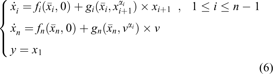
Consider a class of nonlinear system in the following pure-feedback form

where

where v max is a positive but unknown parameter.
Assumption 1
The state variables
Since the unknown functions fi,

where

For the analysis convenience, it is defined that
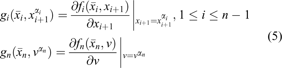
which are unknown nonlinear functions. From equations (4) and (5), equation (1) can be re-expressed as
System coordinate transformation
In the following, it will be shown that the original system (1) can be transformed into the canonical form with respect to the newly defined state variables. 16
Let

The time derivative of z2 is derived as

where

where

where
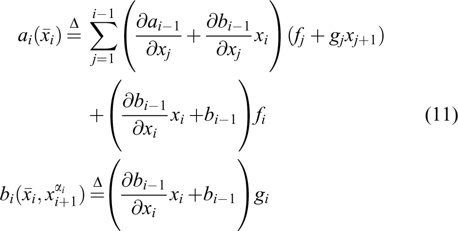
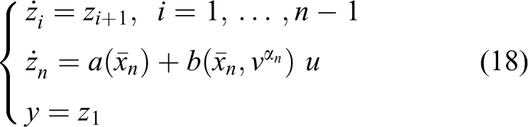
Thus, the pure feedback system (6) can be rewritten in the canonical form with respect to the newly defined state variables as

To proceed the design procedure, the control function
The control objective of this article is to design a dynamic surface sliding-mode controller v(t) for the system (12), such that the system output y can track the desired reference signal yd and all signals in the closed-loop system are bounded.
Nonlinear saturation model
As shown in Figure 1, the control input v(t) ∈ R is the output of the following nonlinear input saturation and u(t) ∈ R is the input of the saturation (practical control signal). The saturation is approximated by a smooth non-affine function defined as
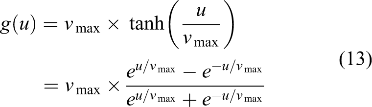
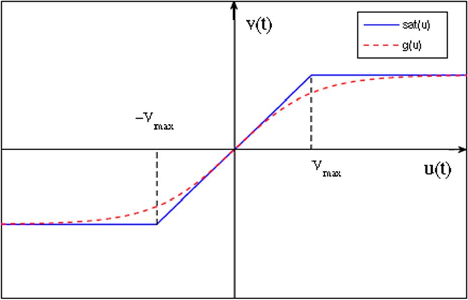
Saturation sat(u) (solid line) and smooth function g(u) (dot line).
Then,

where

where D is the upper bound of |d(u)|.
According to the mean value theorem, 8 there exists a constant ξ with 0 < ξ < 1, such that

where

Substituting equations (17) and (14) into equation (12), we can obtain
where
NN approximation
Due to good capabilities in function approximation, NNs are usually used for the approximation of nonlinear functions. 8,9 The following NN will be used to approximate the continuous function

where

where r 1, r 2, r 3, and r 4 are appropriate parameters, and exp is an exponential function.
Remark 1
The employed NN with sigmoid function represents a class of linearly parameterized approximation methods and can be replaced by any other approximation approaches such as spline functions, RBF functions, or fuzzy systems. However, the structure of the employed NN in this article is simpler than the other NNs that are commonly used in other works. There is no hidden layer in the employed NN, in which five inputs and one output are included and the corresponding weight matrix is 5 × 1.
Controller design
In this section, we will incorporate the DSC and integral sliding mode techniques into a NN-based adaptive control design scheme for the nth-order system described by equation (12). Similar to the traditional backstepping design, the recursive design procedure contains n steps. From step 1 to step n − 1, virtual control
Step 1
In this step, we consider the first equation of equation (12), that is,
Define the tracking error and its sliding surface as

where yd is the desired reference signal and λ is a positive constant.
The derivatives of e and s 1 are

Choose a virtual control

where k1 is a positive constant.
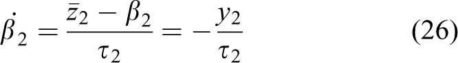
Introduce a new state variable ²2 and let

Define

Substituting equation (25) into equation (24), we can obtain
Step 2
Consider

Let

which is called the second error surface. Then, we have

Choose a virtual control

where k2 is a positive constant.
Again, introducing a new state variable β3 and let

Define

Substituting equation (32) into equation (31), we can obtain

Step i
Consider

Let

which is called the ith error surface. Then, we have

Choose a virtual control

where ki is a positive constant.
Introduce a new state variable βi+1 and let

Define

Substituting equation (39) into equation (38), we can obtain

Step n. The final control law will be derived in this step. Consider

Given a compact set

with

which is called the nth error surface. From equations (41) and (43), we have

Finally, design the final law u as

where

where σ and δ are positive small constants and Γ = ΓT > 0 is a constant matrix.
Stability analysis
In this section, a theorem is provided to show the boundedness of all signals in system (12) and convergence of tracking error e as well as sliding surface s.
Theorem 1
Consider the nonlinear system (12) with unknown input saturation (14), the integral sliding mode surface (21), control law (45), and adaptive learning laws (46). Given any positive number, for all initial conditions satisfying
Proof
Firstly, define the estimation error as

Then, the closed-loop system in the new coordinates, si, βi, and

From equation (48), we have

Besides, we know the fact that

where
Similarly, for

Consider the Lyapunov function candidate

The derivative of the Lyapunov function is
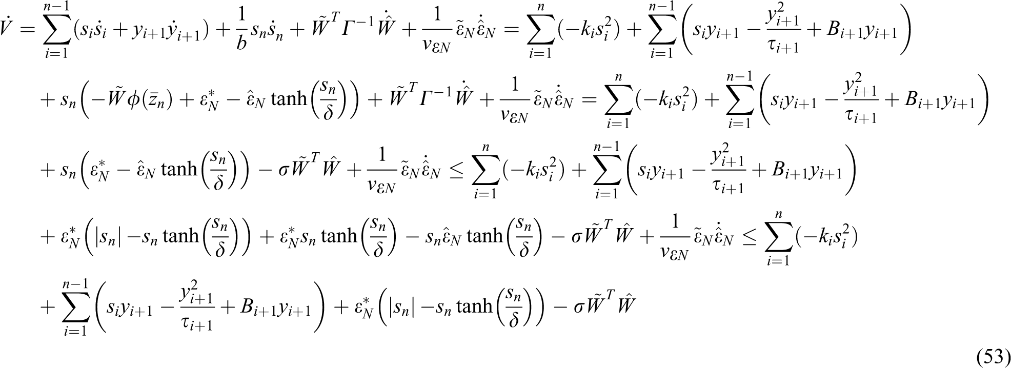
Using the following property with regard to function tanh(.), we have

Using the fact

and substituting equations (54) and (55) into equation (53), we can obtain

Using the fact

we have

Choose
where α0 and η are positive constants and
Remark 2
As pointed out in the study by Li et al.
15
for any B0 > 0 and p > 0, the sets
Noting that, for any positive number η

we can obtain

Hence, we can conclude
Then, the ultimate boundedness of s i is guaranteed, and s i will converge to the following positively invariant set

with
When s1 reaches the positively invariant set γs, it remains inside thereafter. From equation (12), the error dynamics inside γs is

Due to the boundedness of s1 and
Simulations
In order to show the superior tracking performance of the proposed scheme, we consider three different control schemes for comparison: (S1) neural dynamic SMC with saturation compensation; (S2) neural dynamic SMC without saturation compensation; and (S3) neural DSC without saturation compensation. 15
The following four indices are adopted to compare the tracking performance of each control algorithm.
In the following, two simulation examples are adopted for the fair comparison of different control schemes.
Spring mass and damper system
The considered spring mass and damper system represents a class of widely used second-order electromechanical servo systems, such as hydraulic systems, rigid robots, or turntable systems. 22 –24 In those systems, the number of freedom degrees is always equal to the number of control inputs, and thus the controller design is relatively easier.
As shown in Figure 2, a second-order system is described as 7

where y = x1, x1 and x2 are the position and velocity, respectively; m is the mass of the object; k is the stiffness constant of the spring; and c is the damping.

Spring mass and damper system.
According to equation (8), equation (65) can be transformed into

where
In the simulation, two different signal waves are adopted as the desired reference signals, and the system parameters are fixed for various reference signals. The initial states of the system are
Case 1
The input saturation bound is vmax = 14 N. Comparative tracking performance, tracking errors, and control input are shown in Figures 3, 4, and 5, respectively. From Figures 3 and 4, we can see that compared with the proposed S1 method, S2 has the larger overshoot, and S2 and S3 have larger tracking errors. From Figure 5(a), compared with S2 and S3, the control input of S1 is more smooth, and the compensation effect of input saturation is shown in Figure 5(b). From the figures, we can clearly observe the significantly improved performances with the S1.
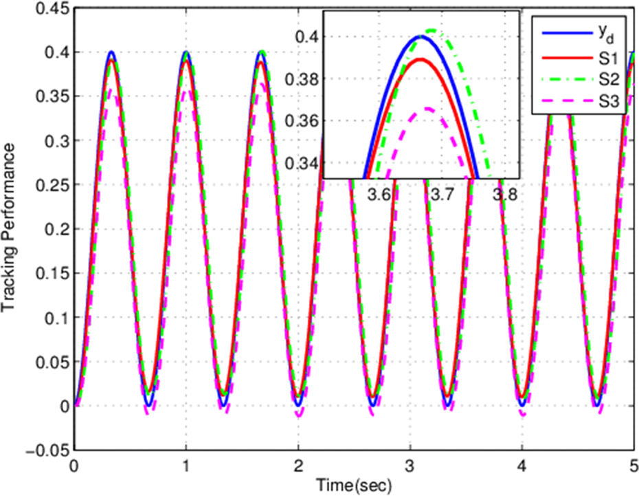
Tracking performance of

Tracking errors of

Control inputs of
In order to compare the control performance, four indices are given in Table 1. From Table 1, we can obtain that S3 controller gives the largest IAV and ISDV, while S2 controller gives the largest IAE and ISDE. The proposed S1 has the smallest IAE, ISDE, IAV, and ISDV, which means it performs best among three controllers. The comparative result from Table 1 is consistent with the Figures 3 to 5.
Comparison for

IAE: integrated absolute error; ISDE: integrated square error; ISDV: integrated square control; IAV: integrated absolute control.
Case 2
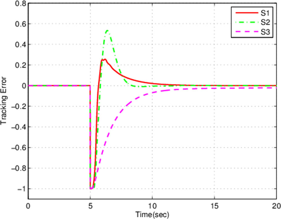
The first reference trajectory is sinusoidal signal, and all parameters are tuned based on this signal. In order to show the high robustness of the proposed method, we give the second reference trajectory (sinusoidal signal with harmonics). The control parameters are set the same as case 1, and the input saturation bound becomes vmax = 6 N, which is more stringent than that of case 1. Comparative tracking performance, tracking errors, and control inputs are shown in Figures 6, 7, and 8, respectively. From Figures 6 and 7, we can see that S2 and S3 have larger tracking errors, while the proposed S1 method achieves the smallest tracking errors and fastest convergence speed. From Figure 8(a), compared with S2 and S3, the control input of S1 is more smooth, and the compensation effect of input saturation is shown in Figure 8(b). In conclusion, S1 has the best performance when tracking the sinusoidal signal with harmonics.
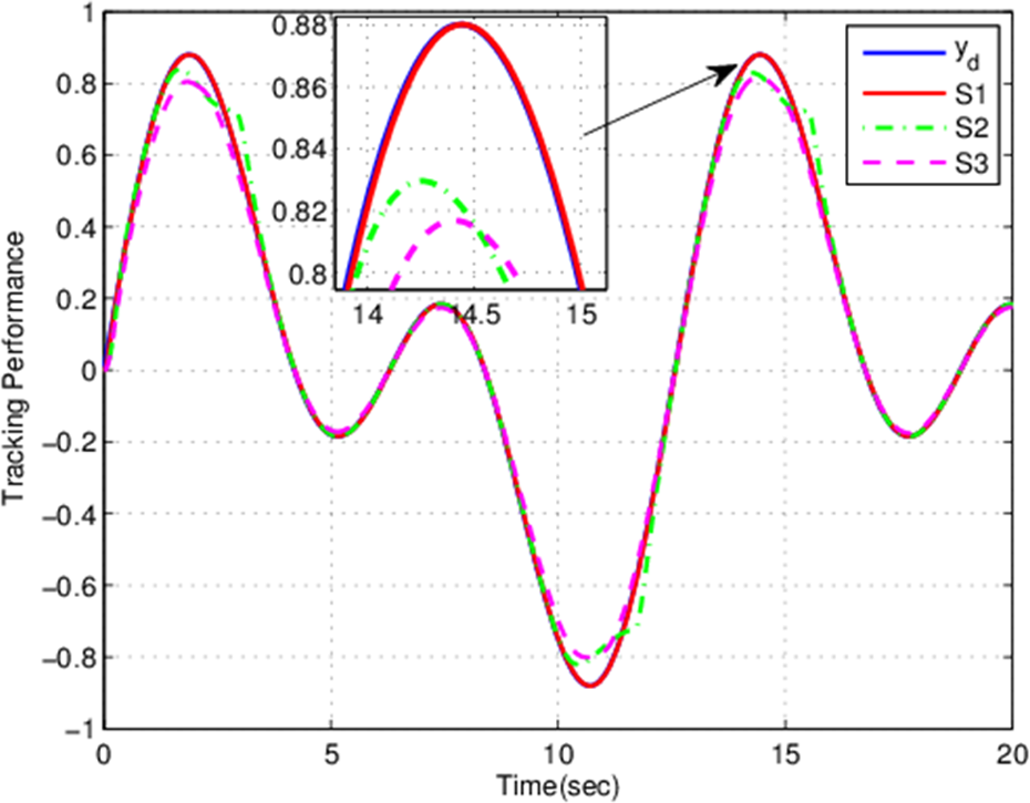
Tracking performance of

Tracking errors of

Control inputs of
In addition, the comparative results of the IAE are shown in Table 2. From Table 2, we can see that the proposed S1 method has the smallest IAE among all the three control schemes. Besides, other three indices (i.e. ISDE, IAV, and ISDV) of the proposed S1 method are also smallest, which means S1 has the smoothness of tracking error and control signal. Therefore, S1 has the best tracking preference, which is consistent with the results given by Figures 6 to 8.
Comparison for

IAE: integrated absolute error; ISDE: integrated square error; ISDV: integrated square control; IAV: integrated absolute control.
Furthermore, the comparative results of IAE for different input saturation values of case 1 and case 2 are shown in Tables 3 and 4, respectively. From Table 3, we can see that the proposed S1 method has the smallest IAE in case 1 compared with S2 and S3, although the input saturation values are changed from 10 to 18. Table 4 shows that for case 2, the proposed S1 scheme with the fixed parameters can still achieve the best tracking performance in the case of various input saturation values. It should be noted that with the input saturation becoming more stringent, the IAE of S2 and S3 will be changed much larger than that of S1. In conclusion, the proposed S1 scheme can achieve a satisfactory tracking performance for different input saturation values.
Comparison of IAE for case 1.

IAE: integrated absolute error.
Comparison of IAE for case 2.
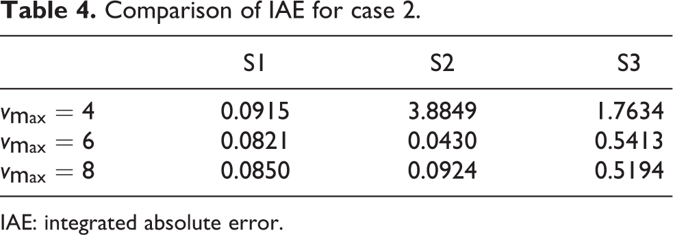
IAE: integrated absolute error.
A single-link flexible-joint robotic manipulator system
In the following, we give the second example, that is, a single-link flexible-joint robotic manipulator system. 25 Due to the introduction of joint flexibility in the robot model, the motion equations become more complicated. In particular, the order of the related dynamics becomes twice that of the rigid robots, and the number of freedom degrees is larger than the number of control inputs, which may lead the control task more difficult.
As shown in Figure 9 (figure 1 in the study by Talole
25
), the mechanical dynamics of the robotic manipulator system can be described as


Schematic of flexible-joint manipulator.
For convenience of the controller design, defining

Let
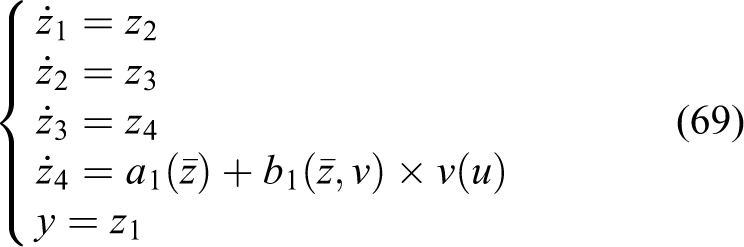
where
According to equation (8), equation (69) can be rewritten as
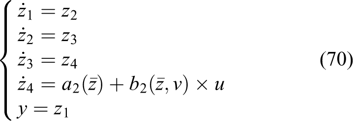
where
In the simulation, two different signal waves are adopted as the desired reference signals, and the system parameters are fixed for various reference signals. The initial states of the system are
Case 3
Step signal yd = 1 is employed as the reference signal.
The input saturation is

Tracking performance of step signal yd = 1.
Tracking errors of step signal yd = 1. (a) Control inputs of three methods. (b) The saturated control v(t) and the practical control u(t) in S1.

Control inputs of step signal yd = 1.
Case 4
Trapezoidal wave is employed as the reference signal.
This reference signal is expressed by

The control parameters are set the same as case 3. Comparative tracking performance, tracking errors, and control inputs are shown in Figures 13, 14 and 15, respectively. The input saturation of S2 or S3 becomes

Tracking performance of trapezoidal wave (equation (71)).

Tracking errors of trapezoidal wave (equation (71)). (a) The saturated control v(t) and the practical control u(t) in S1. (b) Control inputs of three methods.

Control input of trapezoidal wave (equation (71)).
From all the simulation results, we can conclude that compared with S2 and S3, the proposed S1 scheme has the better tracking performance with respect to tracking errors, convergence speed, and control cost.
Conclusion
In this article, an adaptive neural dynamic surface SMC scheme is proposed for uncertain nonlinear systems with unknown input saturation. The non-smooth saturation is transformed into an affine form by defining a non-affine function and using the mean value theorem. One simple NN is employed for nonlinearity approximation, and the approximation error is estimated by an adaptive learning law. By combing the DSC and the integral sliding mode technique, the controller is designed to improve the system robustness, and comparative simulations are given to illustrate the effectiveness of the proposed method.
Footnotes
Declaration of conflicting interests
The author(s) declared no potential conflicts of interest with respect to the research, authorship, and/or publication of this article.
Funding
The author(s) disclosed receipt of the following financial support for the research, authorship, and/or publication of this article: The authors would like to thank the support from the National Natural Science Foundation of China under grant numbers 61403343 and 61433003 and the China Postdoctoral Science Foundation funded project under grant number 2015M580521.