Sage Journals: Discover world-class research

Abstract

Hydraulically driven manipulators face challenges in achieving high-precision tracking control due to their strong nonlinearity, parameter perturbations, and external load disturbances. In response, this article proposes a neural network-based composite control strategy. A radial basis function (RBF) neural network is employed to approximate and compensate for time-varying disturbances. The state-space equations are reformulated to incorporate parameter perturbations as an extended state variable. An Extended State Observer (ESO) is integrated to estimate parameter perturbations for feedforward compensation and observe the system state variables. Subsequently, a composite controller is designed by integrating backstepping and sliding mode control, with the stability of the closed-loop system proven via Lyapunov theory. Finally, simulation results demonstrate that the proposed control strategy exhibits higher control accuracy and superior robustness compared with PID control and traditional neural network-based nonlinear control.

Keywords

Hydraulic servo system manipulator nonlinear control neural network

Introduction

Hydraulically driven manipulators, characterized by fast response and high load-carrying capacity, are widely used in heavy-duty machinery applications such as assembly (ships and aircraft), metallurgy, and national defence.¹ However, their nonlinear characteristics, system parameter perturbations, and varying external disturbances pose significant challenges to high-precision tracking control. Therefore, developing control strategies that balance tracking accuracy and robustness is of great significance. Currently, numerous scholars have proposed various solutions, such as feedback linearization control,² adaptive control,³ sliding mode control,⁴ iterative learning control,⁵ and intelligent control.⁶ Although feedback linearization control offers higher accuracy than PID control, it is limited to scenarios with known system parameters and cannot effectively handle parameter perturbations in hydraulic systems. Adaptive control, while capable of addressing system parameter variations, exhibits weak resistance to external disturbances. Traditional sliding mode control, despite its strong robustness, introduces high-frequency chattering due to the switching nature of sign functions; this chattering is further amplified by the high-pressure characteristics of hydraulic systems, accelerating actuator wear and reducing control accuracy. With the advancement of artificial intelligence and machine learning, iterative learning and intelligent control have been extensively studied. While these strategies perform well for repeatedly operating systems, they struggle to meet the high real-time requirements of hydraulic manipulators in complex single-task operations, as heavy data training causes computational delays. The aforementioned methods either struggle to achieve the coordinated suppression of parameter perturbations and load disturbances, or fail to balance the performance between robustness and chattering suppression. Furthermore, the actual velocity signals required for full-state feedback control are difficult to measure. Even if the measurement is approximated via numerical differentiation of position, it will be corrupted in the presence of system noise. Therefore, there is an urgent need to develop a composite control strategy capable of synergistically addressing multisource uncertainties, so as to achieve fast response and high-precision tracking control of hydraulically driven manipulators.

The extended state observer (ESO) features stable observation performance, capable of confining state observation errors within a bounded range in finite time. Its observation process is equivalent to the fast-varying subsystem of the system,⁷ enabling it to provide usable velocity signals for controller design. In recent years, ESO has been widely applied in fields such as industrial automation control and computer control. Razmjooei et al.⁸ designed a continuous finite-time state observer for electrohydraulic systems to estimate system state variables, ensuring uniformly bounded observation errors. Guo et al.⁹ developed an ESO for online observation of disturbances and velocity signals in pump-controlled electrohydraulic servo systems. However, none of them have addressed the impact of time-varying disturbances on system control. In this article, state-space equations are reformulated to incorporate parameter perturbations as an extended state variable. The ESO is enabled to simultaneously achieve feedforward compensation of system parameters and observation of system states. Backstepping sliding mode control (BSMC) can effectively suppress nonlinear factors, characterized by fast response and insensitivity to parameter perturbations.¹⁰ This method explicitly handles the nonlinear structure of the system through the recursive design of backstepping control, thereby decomposing complex nonlinear systems into manageable subsystems. By embedding sliding mode terms into the control law, it compensates for the defect of backstepping control being sensitive to disturbances; meanwhile, the design of virtual control laws provides continuous reference trajectories for the sliding mode surface, reducing chattering. Additionally, this article uses the hyperbolic tangent function instead of the sign function to compensate for neural network estimation errors, further mitigating chattering caused by sliding mode control. In recent years, radial basis function (RBF) neural networks have attracted significant attention from scholars due to their simple structure, strong generalization ability, and universal approximation property.¹¹ Zhang et al.¹² utilized RBF neural networks to approximate unmodeled dynamics in attitude control systems, achieving effective compensation for model errors and external disturbances. Li et al.¹³ employed RBF neural networks for the accurate estimation of the state of charge of lithium-ion batteries, addressing the challenges of real-time estimation and low accuracy in conventional methods. Feng et al.¹⁴ used three groups of RBF neural networks to approximate uncertain parameters in the manipulator dynamics model, thereby further enhancing the motion control accuracy of the manipulator. RBF neural networks are widely applied in system identification and disturbance estimation due to their fast convergence, strong generalization ability and online weight tuning capability.¹⁵

In this paper, the RBF neural network is employed to focus on real-time estimation of time-varying external disturbances, alleviating the limitation of adaptive control in antidisturbance; the ESO is used to compensate for parameter perturbations and observe system states; the backstepping sliding mode serves as a closed-loop control framework, and combined with hyperbolic tangent function, it mitigates the chattering problem of traditional sliding mode control. Through the synergy of the three, fast response and high-precision tracking of the hydraulic manipulator under multisource uncertainties are achieved.

System description

As shown in Figure 1, the multi-degree-of-freedom hydraulically driven manipulator consists of an actuating mechanism (manipulator joints) and a driving mechanism (servo valves, hydraulic cylinders, power sources, etc.).¹⁶ Subsequently, its mechanical dynamics and hydraulic system models are developed.

Figure 1.

Multi-degree-of-freedom hydraulically driven manipulator.

The dynamic model of the multi-degree-of-freedom manipulator can be expressed as follows¹⁷:

M (q) \ddot{q} + C (q, \dot{q}) \dot{q} + G (q) + F (\dot{q}) = τ - τ_{d}

(1)

where

q, \dot{q}, \ddot{q} \in R^{n}

are the joint angle, angular velocity, and angular acceleration, respectively;

M (q) \in R^{n \times n}

the positive definite inertia matrix of the joint;

C (q, \dot{q}) \in R^{n \times n}

the Coriolis and centrifugal force matrix;

G (q) \in R^{n}

the gravity vector;

F (\dot{q}) \in R^{n}

the joint friction vector;

τ \in R^{n}

the control torque of the manipulator joint; and

τ_{d} \in R^{n}

includes unmodeled terms and external disturbance torques.

The control torque of the manipulator joint can be expressed as equation (2):

τ = h (q) \cdot (A_{1} P_{1} - A_{2} P_{2})

(2)

where

A_{1} = diag (A_{11}, A_{21}, \dots, A_{n 1}) \in R^{n \times n}

A_{2} =

diag (A_{12}, A_{22}, \dots, A_{n 2}) \in R^{n \times n}

;

A_{i 1}

and

A_{i 2}

represent the effective piston areas of the two chambers of each hydraulic cylinder;

i = 1, 2, \cdot \cdot \cdot, n

the index of the joint or actuator;

P_{1} = (P_{11}, P_{21}, \dots, P_{n 1})^{T} \in R^{n}

P_{2} = (P_{12}, P_{22}, \dots, P_{n 2})^{T} \in R^{n}

;

P_{i 1}

and

P_{i 2}

the pressures of the rodless chamber and rod-end chamber of each joint hydraulic cylinder respectively;

h (q) = diag (h_{1}, h_{2}, \dots, h_{n}) \in R^{n \times n}

the effective force arm of each hydraulic cylinder, which can be obtained from the geometric relationship in Figure 2 as equation (3):

h_{i} = \frac{l_{i 1} l_{i 2} \sin (q_{i})}{\sqrt{l_{i 1}^{2} + l_{i 2}^{2} - 2 l_{i 1} l_{i 2} \cos (q_{i})}}, i = 1, 2, \dots, n

(3)

where

l_{i 1}

is the distance between the lower articulation point of the

i t h

hydraulic cylinder and the joint articulation point;

l_{i 2}

is distance between the upper articulation point of the

i t h

hydraulic cylinder and the joint articulation point.

Figure 2.

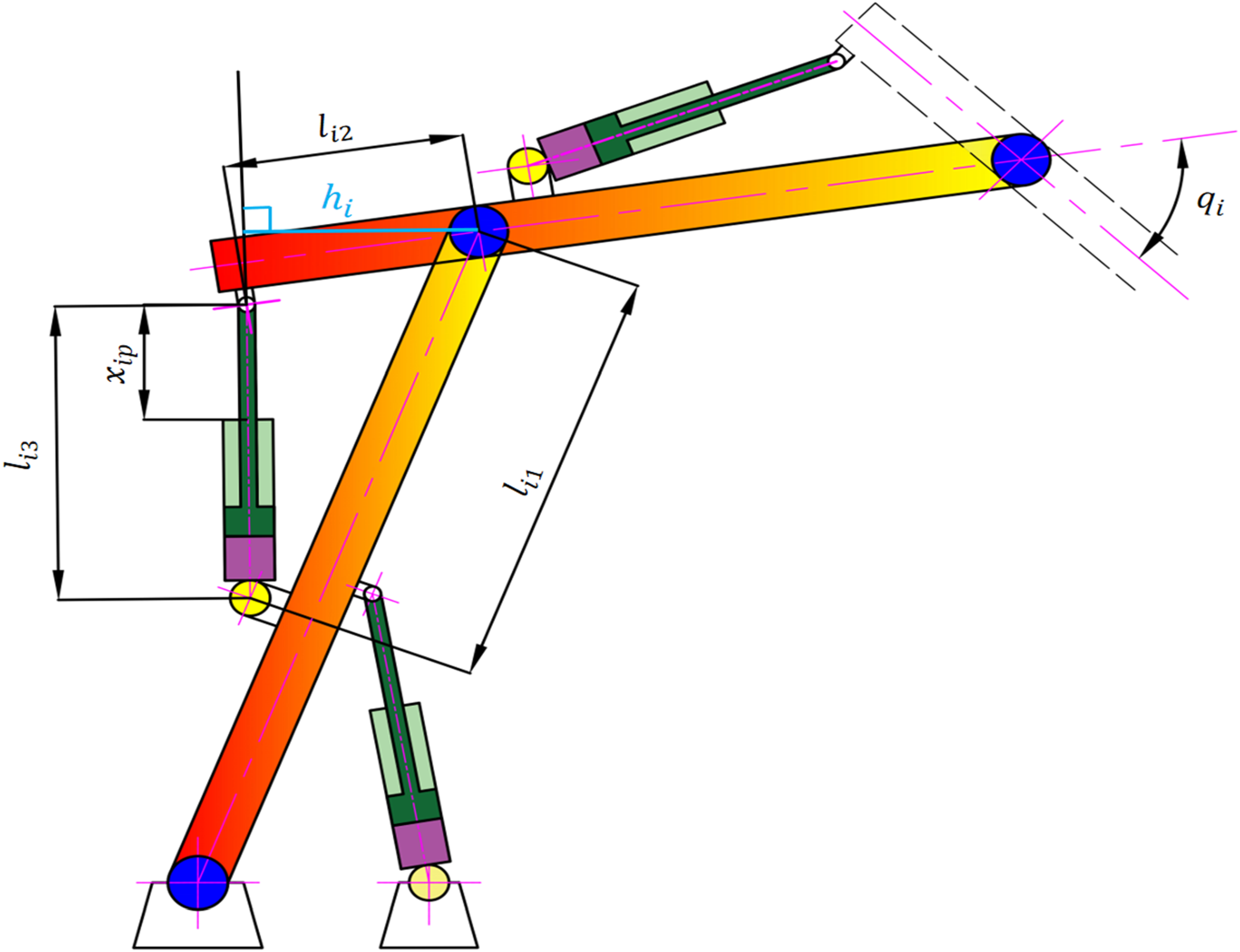
Geometric model of the joint.

The flow continuity equation of the hydraulic cylinder can be described as equation (4):

{\begin{matrix} {\dot{P}}_{1} = β V_{1}^{- 1} (Q_{1} - A_{1} {\dot{x}}_{p} - C_{t} P_{L}) \\ {\dot{P}}_{2} = β V_{2}^{- 1} (A_{2} {\dot{x}}_{p} - Q_{2} + C_{t} P_{L}) \end{matrix}

(4)

where

V_{1} = diag (V_{11}, V_{21}, \dots, V_{n 1}) \in R^{n \times n}

;

V_{2} = diag

(V_{12}, V_{22}, \dots, V_{n 2}) \in R^{n \times n}

;

V_{i 1} = V_{i 01} + A_{i 1} x_{i p}

V_{i 2} = V_{i 02} - A_{i 2} x_{i p}

are the volumes of the two chambers of each hydraulic cylinder,

V_{i 01}

and

V_{i 02}

the initial volumes of the chambers;

x_{p} = (x_{1 p}, x_{2 p}, \dots, x_{n p})^{T} \in R^{n}

the piston displacement of each cylinder;

Q_{1} = (Q_{11}, Q_{21}, \dots, Q_{n 1})^{T} \in R^{n}

;

Q_{2} = (Q_{12}, Q_{22}, \dots, Q_{n 2})^{T} \in R^{n}

;

Q_{i 1}

and

Q_{i 2}

the flow rates of the two chambers of cylinder respectively;

C_{t} = diag (C_{1 t}, C_{2 t}, \dots, C_{n t}) \in R^{n \times n}

the leakage coefficient of the hydraulic cylinder;

P_{L} = (P_{1 L}, P_{2 L}, \dots, P_{n L})^{T} \in R^{n}

;

P_{i L} = P_{i 1} - P_{i 2}

the load pressure; and

β

the effective bulk modulus of the hydraulic oil.

The velocity vector ${\dot{x}}_{p}$ in the actuator space can be expressed by the velocity vector $\dot{q}$ in the joint space¹⁸:

{\dot{x}}_{p} = J_{a} (q) \dot{q}

(5)

where

J_{a} (q) = diag (\frac{\partial x_{1 p}}{\partial q_{1}}, \frac{\partial x_{2 p}}{\partial q_{2}}, \dots, \frac{\partial x_{n p}}{\partial q_{n}}) \in R^{n \times n}

represents the functional relationship of the hydraulic-cylinder velocity vector relative to the corresponding joint-velocity vector.

Since the response speed of the servo valve is much faster than that of the hydraulic cylinder, there is the following proportional relationship¹⁹:

x_{v} = k_{x v} u

(6)

where

x_{v} = (x_{1 v}, x_{2 v}, \dots, x_{n v})^{T} \in R^{n}

is the spool displacement of the servo valve;

k_{x v}

the proportional gain of the servo valve; and

u = (u_{1}, u_{2}, \dots, u_{n})^{T} \in R^{n}

the control input of the servo valve.

The flow equations of the servo valve can be expressed as equation (7):

{\begin{matrix} Q_{1} = C_{d} ω k_{x v} \sqrt{\frac{2}{ρ}} R_{1} u \\ Q_{2} = C_{d} ω k_{x v} \sqrt{\frac{2}{ρ}} R_{2} u \end{matrix}

(7)

where

C_{d}

is the flow coefficient of the orifice in the servo valve;

ω

the area gradient of the orifice; and

ρ

the density of the hydraulic oil;

R_{1} = diag (R_{11}, R_{21}, \dots, R_{n 1}) \in R^{n \times n}, R_{2} = diag (R_{12}, R_{22}, \dots, R_{n 2}) \in R^{n \times n}

where

R_{i 1}

and

R_{i 2}

can be expressed as equation (8):

{\begin{matrix} R_{i 1} = \sqrt{Δ P_{i 1}}, Δ P_{i 1} = {\begin{matrix} P_{S} - P_{i 1}, u_{i} \geq 0 \\ P_{i 1} - P_{r}, u_{i} < 0 \end{matrix} \\ R_{i 2} = \sqrt{Δ P_{i 2}}, Δ P_{i 2} = {\begin{matrix} P_{i 2} - P_{r}, u_{i} \geq 0 \\ P_{S} - P_{i 2}, u_{i} < 0 \end{matrix} \end{matrix}

(8)

where

P_{S}

is the supply oil pressure and

P_{r}

the return oil pressure.

Define the state variable of the system as $x = [x_{1}^{T}, x_{2}^{T}, x_{3}^{T}]^{T}$ , $x_{1} = q$ , $x_{2} = \dot{q}$ , $x_{3} = A_{1} P_{1} - A_{2} P_{2}$ . Combining equations (1), (2), (4), (5), (7), and (8), the dynamic model of the overall hydraulically driven manipulator can be obtained as equation (9):

{\begin{matrix} {\dot{x}}_{1} = x_{2} \\ {\dot{x}}_{2} = M (x_{1})^{- 1} [h (x_{1}) x_{3} - C (x_{1}, x_{2}) x_{2} - G (x_{1}) - F (x_{2})] - g (t) \\ {\dot{x}}_{3} = φ_{1} u - φ_{2} x_{2} - φ_{3} \end{matrix}

(9)

In equation (9),

{\begin{matrix} g (t) = M (x_{1})^{- 1} τ_{d} \\ φ_{1} = β C_{d} ω k_{x v} \sqrt{\frac{2}{ρ}} (A_{1} V_{1}^{- 1} R_{1} + A_{2} V_{2}^{- 1} R_{2}) \\ φ_{2} = β (A_{1}^{2} V_{1}^{- 1} + A_{2}^{2} V_{2}^{- 1}) J_{a} (x_{1}) \\ φ_{3} = β (A_{1} V_{1}^{- 1} + A_{2} V_{2}^{- 1}) C_{t} P_{L} \end{matrix}

(10)

Controller design

Define the system's uncertain parameters as $φ_{z} = {\hat{φ}}_{z} + {\tilde{φ}}_{z} (z = 1, 2, 3)$ , where ${\hat{φ}}_{z}$ denote the nominal values of the parameters and ${\tilde{φ}}_{z}$ the deviations from the nominal values to the true values. Based on this definition, the state-space representation is transformed as equation (11):

{\begin{matrix} {\dot{x}}_{1} = x_{2} \\ {\dot{x}}_{2} = M (x_{1})^{- 1} [h (x_{1}) x_{3} - C (x_{1}, x_{2}) x_{2} - G (x_{1}) - F (x_{2})] - g (t) \\ {\dot{x}}_{3} = {\hat{φ}}_{1} u - {\hat{φ}}_{2} x_{2} - {\hat{φ}}_{2} + λ \end{matrix}

(11)

where auxiliary term

λ

is defined as:

λ = {\tilde{φ}}_{1} u - {\tilde{φ}}_{2} x_{2} - {\tilde{φ}}_{3}

The design block diagram of the controller is illustrated in Figure 3.

1. Design of the RBF neural network

Figure 3.

Block diagram of the controller design concept.

The RBF neural network adopts a three-layer classical topology, comprising an input layer, a hidden layer, and an output layer, as depicted in Figure 4. The dimension of the input layer matches the number of joint angles $x_{1}$ and angular velocities $x_{2}$ of the system, while the dimension of the output layer aligns with the number of joint disturbances $g (t)$ .

Figure 4.

Structure of the radial basis function (RBF) neural network.

Its activation function is the Gaussian function, and the fitting formula is shown as equation (12):

{\begin{matrix} h_{j} \circ = \exp (- \frac{{‖ x_{n} - c_{j} ‖}^{2}}{2 b_{j}^{2}}) j = 1, 2, \dots, m \\ g (t) = W^{* T} H + ε_{R} \end{matrix}

(12)

where j is the index of neurons in the hidden layer.;

x_{n}

the input vector of the neural network;

H = [h_{1}^{o}, h_{2}^{o}, \dots, h_{m}^{o}]^{T} \in R^{m}

the output of Gaussian function;

c_{j}

the center vector of the Gaussian basis function;

b_{j}

the width of this Gaussian basis function;

W^{* T} \in R^{n \times m}

the ideal weight matrix;

g (t)

the target function vector to be approximated;

ε_{R} \in R^{n}

the network approximation error vector, and

‖ ε_{R} ‖ \leq ε_{N}

The estimation vector of $g (t)$ is shown as equation (13):

\hat{g} (t) = {\hat{W}}^{T} H

(13)

where

{\hat{W}}^{T}

is the estimated matrix of weights.

Define the estimation error as equation (14):

\tilde{g} (t) = g (t) - \hat{g} (t) = W^{* T} H + ε_{R} - {\hat{W}}^{T} H = {\tilde{W}}^{T} H + ε_{R}

(14)

where

{\tilde{W}}^{T}

is the error matrix of weights, which can be defined as equation (15):

{\tilde{W}}^{T} = W^{* T} - {\hat{W}}^{T}

(15)

2. Design of ESO

Let $λ = x_{4}$ , and its time-varying rate is denoted as $d (t)$ with $‖ d (t) ‖ \leq d_{max}$ . Then, the extended state-space form of equation (11) is given by equation (16):

{\begin{matrix} {\dot{x}}_{1} = x_{2} \\ {\dot{x}}_{2} = M (x_{1})^{- 1} [h (x_{1}) x_{3} - C (x_{1}, x_{2}) x_{2} - G (x_{1}) - F (x_{2})] - g (t) \\ {\dot{x}}_{3} = {\hat{φ}}_{1} u - {\hat{φ}}_{2} x_{2} - {\hat{φ}}_{3} + x_{4} \\ {\dot{x}}_{4} = d (t) \end{matrix}

(16)

Based on equation (16), the ESO is designed as equation (17):

{\begin{matrix} {\dot{\hat{x}}}_{1} = {\hat{x}}_{2} + α_{1} w_{0} I_{n} (x_{1} - {\hat{x}}_{1}) \\ {\dot{\hat{x}}}_{2} = M ({\hat{x}}_{1})^{- 1} [h ({\hat{x}}_{1}) {\hat{x}}_{3} - C ({\hat{x}}_{1}, {\hat{x}}_{2}) {\hat{x}}_{2} - G ({\hat{x}}_{1}) - F ({\hat{x}}_{2})] - \hat{g} (t) + α_{2} w_{0}^{2} I_{n} (x_{1} - {\hat{x}}_{1}) \\ {\dot{\hat{x}}}_{3} = {\hat{φ}}_{1} u - {\hat{φ}}_{2} {\hat{x}}_{2} - {\hat{φ}}_{3} + {\hat{x}}_{4} + α_{3} w_{0}^{3} I_{n} (x_{1} - {\hat{x}}_{1}) \\ {\dot{\hat{x}}}_{4} = α_{4} w_{0}^{4} I_{n} (x_{1} - {\hat{x}}_{1}) \end{matrix}

(17)

where

{\hat{x}}_{q} \in R^{n} (q = 1, 2, 3, 4)

is the observed value of

x_{q} (q = 1, 2, 3, 4)

and

w_{0}

the observer bandwidth.

Define the state error as ${\tilde{x}}_{q} = x_{q} - {\hat{x}}_{q}$ . Then, the state equation of the observation error system is given by:

{\begin{matrix} {\dot{\tilde{x}}}_{1} = {\tilde{x}}_{2} - α_{1} w_{0} I_{n} {\tilde{x}}_{1} \\ {\dot{\tilde{x}}}_{2} = δ (\tilde{x}) - {\tilde{W}}^{T} H - ε_{R} - α_{2} w_{0}^{2} I_{n} {\tilde{x}}_{1} \\ {\dot{\tilde{x}}}_{3} = - {\hat{φ}}_{2} {\tilde{x}}_{2} + {\tilde{x}}_{4} - α_{3} w_{0}^{3} I_{n} {\tilde{x}}_{1} \\ {\dot{\tilde{x}}}_{4} = d (t) - α_{4} w_{0}^{4} I_{n} {\tilde{x}}_{1} \end{matrix}

(18)

where

δ (\tilde{x})

is denoted as the difference of the function

M (x_{1})^{- 1} [h (x_{1}) x_{3} - C (x_{1}, x_{2}) x_{2} - G (x_{1}) - F (x_{2})]

before and after observation; based on multiple sets of simulation results, it can be simplified as

δ (\tilde{x}) = k_{0} I_{n} {\tilde{x}}_{3}

for brevity, where

k_{0} \approx 1.0875

Let $ε_{q} = \frac{{\tilde{x}}_{q}}{w_{0}^{q - 1}}$ , $ε = (ε_{1}, ε_{2}, ε_{3}, ε_{4})^{T}$ . Then, the state equation of the observation error is:

\dot{ε} = w_{0} A ε + \frac{B_{1}}{w_{0}} ({\tilde{W}}^{T} H + ε_{R}) + \frac{B_{2}}{w_{0}} {\hat{φ}}_{2} ε_{2} + \frac{B_{3}}{w_{0}^{3}} d (t)

(19)

where

ε = (ε_{1}, ε_{2}, ε_{3}, ε_{4})^{T}

A = (\begin{matrix} - α_{1} I_{n} I_{n} 0 0 \\ - α_{2} I_{n} 0 k_{0} I_{n} 0 \\ - α_{3} I_{n} 0 0 I_{n} \\ - α_{4} I_{n} 0 0 0 \end{matrix})

B_{1} = (0 - I_{n} 00)^{T}

B_{2} = (00 - I_{n} 0)^{T}

B_{3} = (000 I_{n})^{T}

. Reasonably design

α_{1}, α_{2}, α_{3}, α_{4}

to make matrix

A

a Hurwitz matrix. Then there is the theorem: for any given symmetric positive-definite matrix

Q

, there exists a symmetric positive-definite matrix

P

such that equation (20) is satisfied:

A^{T} P + P A = - Q

(20)

3. Controller design based on backstepping sliding mode

Define the state errors of the system as equation (21):

{\begin{matrix} e_{1} = x_{1} - x_{1 d} \\ e_{2} = x_{2} - x_{2 d} \\ e_{3} = x_{3} - x_{3 d} \end{matrix}

(21)

where

x_{1 d}

is the command angle signal;

x_{2 d}

and

x_{3 d}

the virtual control quantities for

x_{2}

and

x_{3}

respectively.

Define the Lyapunov function $V_{1}$ as equation (22):

V_{1} = \frac{1}{2} e_{1}^{T} e_{1}

(22)

Deriving it yields:

{\dot{V}}_{1} = e_{1}^{T} {\dot{e}}_{1} = e_{1}^{T} (x_{2} - {\dot{x}}_{1 d})

(23)

To make ${\dot{V}}_{1}$ negative definite, design the virtual control quantity $x_{2 d}$ as equation (24):

x_{2 d} = - k_{1} e_{1} + {\dot{x}}_{1 d}

(24)

Define the Lyapunov function $V_{2}$ as equation (25):

V_{2} = V_{1} + \frac{1}{2} e_{2}^{T} e_{2}

(25)

Deriving it yields:

{\dot{V}}_{2} = {\dot{V}}_{1} + e_{2}^{T} ({\dot{x}}_{2} - {\dot{x}}_{2 d}) = - k_{1} e_{1}^{T} e_{1} + e_{1}^{T} e_{2} + e_{2}^{T} {M {(x_{1})}^{- 1} [\begin{matrix} h (x_{1}) x_{3} - C (x_{1}, x_{2}) x_{2} \\ - G (x_{1}) - F (x_{2}) \end{matrix}] - g (t) - {\dot{x}}_{2 d}}

(26)

Design the virtual control quantity $x_{3 d}$ using the observed value ${\hat{x}}_{2}$ from ESO, which is given as equation (27):

\begin{aligned} x_{3 d} = h (x_{1})^{- 1} {M (x_{1}) [- k_{2} {\hat{e}}_{2} + \hat{g} (t) + {\hat{\dot{x}}}_{2 d}] \\ + C (x_{1}, {\hat{x}}_{2}) {\hat{x}}_{2} + G (x_{1}) + F ({\hat{x}}_{2})} \end{aligned}

(27)

where

{\hat{\dot{x}}}_{2 d}

and

{\hat{e}}_{2}

are defined as equations (28) and (29):

{\hat{\dot{x}}}_{2 d} = - k_{1} ({\hat{x}}_{2} - {\dot{x}}_{1 d}) + {\ddot{x}}_{1 d}

(28)

{\hat{e}}_{2} = {\hat{x}}_{2} - x_{2 d}

(29)

Define the sliding mode function as equation (30):

s = c_{1} e_{1} + c_{2} e_{2} + e_{3}

(30)

All of $k_{1}$ , $k_{2} c_{1}$ , and $c_{2}$ are positive constants.

Differentiating equation (30), we can get equation (31):

\begin{aligned} \dot{s} = & c_{1} {\dot{e}}_{1} + c_{2} {\dot{e}}_{2} + {\dot{e}}_{3} \\ = & c_{1} {\dot{e}}_{1} + c_{2} {M {(x_{1})}^{- 1} [\begin{matrix} h (x_{1}) x_{3} - C (x_{1}, x_{2}) x_{2} \\ - G (x_{1}) - F (x_{2}) \end{matrix}] - g (t) - {\dot{x}}_{2 d}} + ({\hat{φ}}_{1} u - {\hat{φ}}_{2} x_{2} - {\hat{φ}}_{3} + x_{4} - {\dot{x}}_{3 d}) \end{aligned}

(31)

To overcome the chattering problem caused by the discontinuity of the switching function, the $\tanh (s)$ function is used to replace the $sgn (s)$ function, and the control law is designed as equation (32):

u = {\hat{φ}}_{1}^{- 1} {\begin{matrix} - k_{g} \hat{s} - ε_{N} \tanh (s) + {\hat{φ}}_{2} {\hat{x}}_{2} + {\hat{φ}}_{3} - {\hat{x}}_{4} + {\dot{x}}_{3 d} - c_{1} {\hat{\dot{e}}}_{1} \\ - c_{2} {M {(x_{1})}^{- 1} [\begin{matrix} h (x_{1}) {\hat{x}}_{3} - C (x_{1}, {\hat{x}}_{2}) {\hat{x}}_{2} \\ - G (x_{1}) - F ({\hat{x}}_{2}) \end{matrix}] - \hat{g} (t) - {\hat{\dot{x}}}_{2 d}} \end{matrix}}

(32)

where

{\hat{\dot{e}}}_{1} = {\hat{x}}_{2} - {\dot{x}}_{1 d}

. Define the estimated value of

s

\hat{s} = c_{1} e_{1} + c_{2} {\hat{e}}_{2} + {\hat{e}}_{3}

, where

{\hat{e}}_{3} = {\hat{x}}_{3} - x_{3 d}

; the estimation error

\tilde{s} = s - \hat{s} = c_{2} {\tilde{x}}_{2} + {\tilde{x}}_{3}

, then we can get equation (33):

\hat{s} = s - c_{2} {\tilde{x}}_{2} - {\tilde{x}}_{3}

(33)

Substitute equations (33) into (32) and then substitute the result into equation (31), we can get equation (34):

\begin{aligned} \begin{matrix} \dot{s} = (c_{1} I_{n} + c_{2} I_{n} - {\hat{φ}}_{2} + c_{2} k_{g} I_{n}) w_{0} ε_{2} \end{matrix} \\ + (k_{g} I_{n} + c_{2} k_{0} I_{n}) w_{0}^{2} ε_{3} + w_{0}^{3} ε_{4} - k_{g} s \\ - c_{2} ({\tilde{W}}^{T} H + ε_{R}) - ε_{N} \tanh (s) \end{aligned}

(34)

Design the weight adaptive law of the RBF neural network as equation (35):

\dot{\hat{W}} = (- e_{2}^{T} + ε^{T} P \frac{B_{1}}{w_{0}} - c_{2} s^{T}) H - \hat{W}

(35)

4. Proof of system stability

Lemma 1:

For the neural network weight error $\tilde{W} = W^{*} - \hat{W}$ , the following inequality holds:

2 χ t r {\hat{W} {\tilde{W}}^{T}} \leq - χ ‖ \tilde{W} ‖^{2} + χ ‖ W^{*} ‖^{2}

(36)

where

χ

is a positive constant.

Lemma 2:

For the hyperbolic tangent function, the following inequality holds:

- s^{T} \tanh (s) \leq n μ - ‖ s ‖

(37)

where

μ

is the chattering tradeoff coefficient.

Define the final Lyapunov function V as equation (38):

V = V_{2} + \frac{1}{2} ε^{T} P ε + \frac{1}{2} s^{T} s + \frac{1}{2} {\tilde{W}}^{T} \tilde{W}

(38)

It is straightforward to verify that equation (38) is a positive definite function. By differentiating equation (38), we derive equation (39):

\dot{V} = {\dot{V}}_{2} + ε^{T} P \dot{ε} + s^{T} \dot{s} - {\tilde{W}}^{T} \dot{\hat{W}}

(39)

Substitute equations (19), (26), (34), and (35) into equation (39), and then we can get equation (40):

\begin{aligned} \dot{V} = & - k_{1} e_{1}^{T} e_{1} - k_{2} e_{2}^{T} {\hat{e}}_{2} + e_{1}^{T} e_{2} + k_{1} w_{0} e_{2}^{T} ε_{2} + e_{2}^{T} M (x_{1})^{- 1} h (x_{1}) e_{3} - e_{2}^{T} ε_{R} + ε^{T} P w_{0} A ε + ε^{T} P \frac{B_{2}}{w_{0}} {\hat{φ}}_{2} ε_{2} + ε^{T} P \frac{B_{1}}{w_{0}} ε_{R} \\ + ε^{T} P \frac{B_{3}}{w_{0}^{3}} d (t) + s^{T} [\begin{matrix} (c_{1} I_{n} + c_{2} I_{n} - {\hat{φ}}_{2} + c_{2} k_{g} I_{n}) w_{0} ε_{2} + (k_{g} I_{n} + c_{2} k_{0} I_{n}) w_{0}^{2} ε_{3} \\ + w_{0}^{3} ε_{4} - k_{g} s - c_{2} ε_{R} - ε_{N} \tanh (s) \end{matrix}] + {\tilde{W}}^{T} \hat{W} \end{aligned}

(40)

Here, we let $\dot{V} = {\dot{V}}_{a} + {\dot{V}}_{b}$ , where

{\dot{V}}_{a} = - k_{1} e_{1}^{T} e_{1} - k_{2} e_{2}^{T} {\hat{e}}_{2} + e_{1}^{T} e_{2} + k_{1} w_{0} e_{2}^{T} ε_{2} + e_{2}^{T} M (x_{1})^{- 1} h (x_{1}) e_{3} - e_{2}^{T} ε_{R}

(41)

\begin{aligned} {\dot{V}}_{b} = & ε^{T} P w_{0} A ε + ε^{T} P \frac{B_{2}}{w_{0}} {\hat{φ}}_{2} ε_{2} + ε^{T} P \frac{B_{1}}{w_{0}} ε_{R} + ε^{T} P \frac{B_{3}}{w_{0}^{3}} d (t) \\ + & s^{T} [\begin{matrix} (c_{1} I_{n} + c_{2} I_{n} - {\hat{φ}}_{2} + c_{2} k_{g} I_{n}) w_{0} ε_{2} + (k_{g} I_{n} + c_{2} k_{0} I_{n}) w_{0}^{2} ε_{3} \\ + w_{0}^{3} ε_{4} - k_{g} s - c_{2} ε_{R} - ε_{N} \tanh (s) \end{matrix}] + {\tilde{W}}^{T} \hat{W} \end{aligned}

(42)

By the properties of the manipulator inertia matrix²⁰ (i.e. $M (x_{1})$ is positive definite) and the boundedness of $h (x_{1})$ , we derive the following bound:

e_{2}^{T} M (x_{1})^{- 1} h (x_{1}) e_{3} \leq L ‖ e_{2} ‖ ‖ e_{3} ‖

(43)

where L is a positive constant.

Applying Young's inequality, equation (41) can be rewritten as equation (44):

\begin{aligned} {\dot{V}}_{a} \leq - & k_{1} e_{1}^{T} e_{1} + \frac{{‖ e_{1} ‖}^{2}}{2 σ_{2}} + \frac{σ_{2} {‖ e_{2} ‖}^{2}}{2} + \frac{k_{1}^{2} {‖ e_{2} ‖}^{2}}{2 σ_{3}} + \frac{σ_{3} {‖ {\tilde{x}}_{2} ‖}^{2}}{2} + \frac{k_{2}^{2} {‖ e_{2} ‖}^{2}}{2 σ_{4}} \\ + \frac{σ_{4} {‖ {\hat{e}}_{2} ‖}^{2}}{2} + \frac{L^{2} {‖ e_{2} ‖}^{2}}{2 σ_{1}} + \frac{σ_{1} {‖ e_{3} ‖}^{2}}{2} + \frac{{‖ e_{2} ‖}^{2}}{2 σ_{5}} + \frac{σ_{5} ε_{N}^{2}}{2} \\ = & - (k_{1} - \frac{1}{2 σ_{2}}) ‖ e_{1} ‖^{2} + (\frac{σ_{2}}{2} + \frac{k_{1}^{2}}{2 σ_{3}} + \frac{k_{2}^{2}}{2 σ_{4}} + \frac{L^{2}}{2 σ_{1}} + \frac{1}{2 σ_{5}}) ‖ e_{2} ‖^{2} \\ + \frac{σ_{3} {‖ {\tilde{x}}_{2} ‖}^{2}}{2} + \frac{σ_{4} {‖ {\hat{e}}_{2} ‖}^{2}}{2} + \frac{σ_{1} {‖ e_{3} ‖}^{2}}{2} + \frac{σ_{5} ε_{N}^{2}}{2} \end{aligned}

(44 )

where $σ_{c} (c = 1, 2, 3, 4, 5)$ are positive constants.

If appropriate parameters $σ_{c}$ , $k_{1}$ , and $k_{2}$ are selected to satisfy condition r:

{\begin{matrix} k_{1} - \frac{1}{2 σ_{2}} > 0 \\ σ_{3} ‖ {\tilde{x}}_{2} ‖^{2} + σ_{4} ‖ {\hat{e}}_{2} ‖^{2} + σ_{1} ‖ e_{3} ‖^{2} \leq α ‖ e_{2} ‖^{2}, (α > 0) \\ \frac{σ_{2}}{2} + \frac{k_{1}^{2}}{2 σ_{3}} + \frac{k_{2}^{2}}{2 σ_{4}} + \frac{L^{2}}{2 σ_{1}} + \frac{1}{2 σ_{5}} < k_{1} - \frac{1}{2 σ_{2}} - \frac{σ_{5} ε_{N}^{2}}{2 {‖ e_{2} ‖}^{2}} \end{matrix}

(45)

then, when

e_{2} \neq 0

, equation (46) holds:

β_{2} + ψ < β_{1} - \frac{σ_{5} ε_{N}^{2}}{2 {‖ e_{2} ‖}^{2}}

(46)

where

β_{1} = k_{1} - \frac{1}{2 σ_{2}}; β_{2} = \frac{σ_{2}}{2} + \frac{k_{1}^{2}}{2 σ_{3}} + \frac{k_{2}^{2}}{2 σ_{4}} + \frac{L^{2}}{2 σ_{1}} + \frac{1}{2 σ_{5}}; ψ = \frac{σ_{3} {‖ {\tilde{x}}_{2} ‖}^{2} + σ_{4} {‖ {\hat{e}}_{2} ‖}^{2} + σ_{1} {‖ e_{3} ‖}^{2}}{2 {‖ e_{2} ‖}^{2}}

Let $β_{3} = min {β_{1}, β_{1} - β_{2} - ψ - \frac{σ_{5} ε_{N}^{2}}{2 {‖ e_{2} ‖}^{2}}}$ , and then we can obtain:

{\dot{V}}_{a} \leq - β_{3} ({‖ e_{1} ‖}^{2} + {‖ e_{2} ‖}^{2}) = - β_{3} ‖ e ‖^{2} \leq 0

(47)

By applying Lemma 1 and Lemma 2, equation (42) can be rewritten as equation (48):

\begin{aligned} {\dot{V}}_{b} \leq - & \frac{λ_{min} (Q)}{2} w_{0} ‖ ε ‖^{2} + λ_{max} (P \frac{B_{2}}{w_{0}} {\hat{φ}}_{2}) ‖ ε ‖^{2} + \frac{λ_{max} (P \frac{B_{1}}{w_{0}})}{2} ‖ ε ‖^{2} + \frac{λ_{max} (P \frac{B_{3}}{w_{0}^{3}})}{2} ‖ ε ‖^{2} + \frac{1}{2} ‖ ε ‖^{2} \\ + \frac{w_{0}^{2} λ_{max} (c_{1} I_{n} + c_{2} I_{n} - {\hat{φ}}_{2} + c_{2} k_{g} I_{n})}{2} ‖ s ‖^{2} + \frac{w_{0}^{4} λ_{max} (k_{g} I_{n} + c_{2} k_{0} I_{n})}{2} ‖ s ‖^{2} + \frac{w_{0}^{6}}{2} ‖ s ‖^{2} - k_{g} ‖ s ‖^{2} \\ + \frac{c_{2}^{2}}{2} ‖ s ‖^{2} + \frac{ε_{N}^{2} n}{2} ‖ s ‖^{2} + \frac{μ n ε_{N}}{2} - \frac{{‖ \tilde{W} ‖}^{2}}{2} + \frac{{‖ W * ‖}^{2}}{2} + \frac{d_{max}^{2}}{2} + \frac{ε_{N}^{2}}{2} \end{aligned}

(48)

where

λ_{min} (\cdot)

and

λ_{max} (\cdot)

denote the minimum and maximum eigenvalues of the matrix, respectively.

Define the matrix $η$ and parameters $γ$ , $κ$ , and $ζ$ as equations (49) to (52):

η = (‖ ε_{1} ‖, ‖ ε_{2} ‖, ‖ ε_{3} ‖, ‖ ε_{4} ‖, ‖ s ‖)^{T}

(49)

γ = \frac{λ_{min} (Q)}{2} w_{0} - λ_{max} (P \frac{B_{2}}{w_{0}} {\hat{φ}}_{2}) - \frac{λ_{max} (P \frac{B_{1}}{w_{0}})}{2} - \frac{λ_{max} (P \frac{B_{3}}{w_{0}^{3}})}{2} - \frac{1}{2}

(50)

κ = k_{g} - \frac{w_{0}^{2} λ_{max} (c_{1} I_{n} + c_{2} I_{n} - {\hat{φ}}_{2} + c_{2} k_{g} I_{n})}{2} - \frac{w_{0}^{4} λ_{max} (k_{g} I_{n} + c_{2} k_{0} I_{n})}{2} - \frac{w_{0}^{6}}{2} - \frac{c_{2}^{2}}{2} - \frac{ε_{N}^{2} n}{2}

(51)

ζ = \frac{ε_{N}^{2}}{2} + \frac{μ n ε_{N}}{2} + \frac{{‖ W * ‖}^{2}}{2} + \frac{d_{max}^{2}}{2}

(52)

Accordingly, equation (48) can be recast into the following form:

{\dot{V}}_{b} \leq - η^{T} Λ η - \frac{{‖ \tilde{W} ‖}^{2}}{2} + ζ

(53)

where the matrix

Λ

is defined as

Λ = (\begin{matrix} γ 0 0 0 0 \\ 0 γ 0 0 0 \\ 00 γ 0 0 \\ 000 γ 0 \\ 0000 κ \end{matrix})

. By designing appropriate matrices

Q

and control parameters to ensure

Λ

is positive definite, we deduce the following chain of inequalities:

\begin{aligned} {\dot{V}}_{b} & \leq - λ_{min} (Λ) ({‖ ε ‖}^{2} + {‖ s ‖}^{2}) - \frac{{‖ \tilde{W} ‖}^{2}}{2} + ζ \\ \leq - λ_{min} (Λ) (\frac{1}{λ_{max} (P)} ε^{T} P ε + {‖ s ‖}^{2}) - \frac{{‖ \tilde{W} ‖}^{2}}{2} + ζ \\ \leq - τ V_{b} + ζ \end{aligned}

(54)

In equation (54), $V_{b}$ is defined as $V_{b} = \frac{1}{2} ε^{T} P ε + \frac{1}{2} s^{T} s + \frac{1}{2} {\tilde{W}}^{T} \tilde{W}$ and the parameter $τ$ (denoting the exponential convergence rate) is given by: $τ = 2 min {\frac{λ_{min} (Λ)}{λ_{max} (P)}, λ_{min} (Λ), \frac{1}{2}}$

From the above derivation, we establish the inequality:

V_{b} (t) \leq V_{b} (0) \exp (- τ t) + \frac{ζ}{τ} [1 - \exp (- τ t)]

(55)

Finally, by the decomposition $\dot{V} = {\dot{V}}_{a} + {\dot{V}}_{b}$ , it follows that the proposed controller (i.e. equations (13), (32), and (35)) guarantees the uniform ultimate boundedness of the system in the Lyapunov sense.

Analysis of the simulation process and comparison of result

Simulation process

To verify the effectiveness of the proposed control strategy, this chapter takes a dual-joint system as an example and establishes a co-simulation platform with MATLAB/Simulink and AMESIM.

The structure of the system's dynamic model is as follows:

\begin{aligned} M (q) = [\begin{matrix} M_{11} M_{12} \\ M_{21} M_{22} \end{matrix}], C (q, \dot{q}) = [\begin{matrix} C_{11} C_{12} \\ C_{21} C_{22} \end{matrix}], G (q) = [\begin{matrix} G_{1} \\ G_{2} \end{matrix}], F (\dot{q}) = [\begin{matrix} f_{1} \\ f_{2} \end{matrix}], τ_{d} = [\begin{matrix} τ_{1 d} \\ τ_{2 d} \end{matrix}] \end{aligned}

, where

\begin{aligned} {\begin{matrix} M_{11} = (m_{1} + m_{2}) L_{1}^{2} + m_{2} L_{2}^{2} + 2 m_{2} L_{1} L_{2} \cos (q_{2}) + I_{1} + I_{2} \\ M_{22} = m_{2} L_{2}^{2} + I_{2} \\ M_{21} = m_{2} L_{2}^{2} + m_{2} L_{1} L_{2} \cos (q_{2}) + I_{2} \\ M_{12} = M_{21} \end{matrix} \\ {\begin{matrix} C_{11} = - m_{2} L_{1} L_{c 2} \sin (q_{2}) {\dot{q}}_{2} \\ C_{12} = - m_{2} L_{1} L_{c 2} \sin (q_{2}) ({\dot{q}}_{1} + {\dot{q}}_{2}) \\ C_{21} = m_{2} L_{1} L_{c 2} \sin (q_{2}) {\dot{q}}_{1} \\ C_{22} = 0 \end{matrix} \\ {\begin{matrix} G_{1} = (m_{1} L_{c 1} + m_{2} L_{1}) g \cos (q_{1}) + m_{2} L_{c 2} g \cos (q_{1} + q_{2}) \\ G_{2} = m_{2} L_{c 2} g \cos (q_{1} + q_{2}) \end{matrix} \\ {\begin{matrix} f_{1} = f_{c 1} sgn ({\dot{q}}_{1}) + f_{v 1} {\dot{q}}_{1} \\ f_{2} = f_{c 2} sgn ({\dot{q}}_{2}) + f_{v 2} {\dot{q}}_{2} \end{matrix} \end{aligned}

$L_{i}$ denotes the length of the $i t h$ link; $m_{i}$ the mass of the $i t h$ link; $L_{c i}$ the distance from the center of mass of the $i t h$ link to the $i t h$ joint rotation axis; $I_{i}$ the moment of inertia of the $i t h$ link about the joint axis; g the gravitational acceleration; $f_{c i}$ the Coulomb friction coefficient; and $f_{v i}$ the viscous friction coefficient.

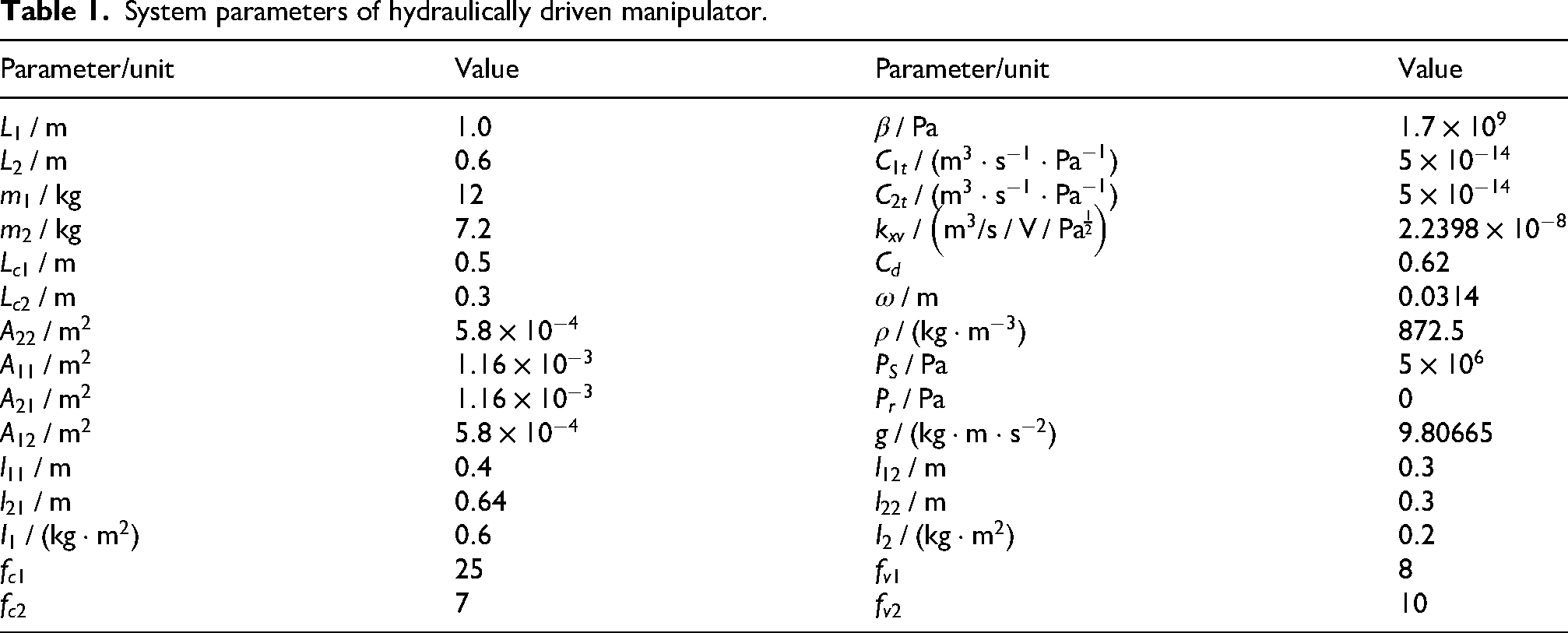
In AMESIM, an external disturbance torque is applied to the model, and the effects of leakage and friction in the hydraulic system on the system performance are considered. In the MATLAB/Simulink model, displacement command signals are input, control algorithms are implemented, and data acquisition is carried out with the acquisition period set to 0.001s. To better approximate real operating conditions, white noise modules are added to each sensor output. Parameters are listed in Table 1.

Table 1.

System parameters of hydraulically driven manipulator.

Parameter/unit	Value	Parameter/unit	Value
$L_{1} / m$	$1.0$	$β / Pa$	$1.7 \times 10^{9}$
$L_{2} / m$	$0.6$	$C_{1 t} / (m^{3} \cdot s^{- 1} \cdot {Pa}^{- 1})$	$5 \times 10^{- 14}$
$m_{1} / kg$	$12$	$C_{2 t} / (m^{3} \cdot s^{- 1} \cdot {Pa}^{- 1})$	$5 \times 10^{- 14}$
$m_{2} / kg$	$7.2$	$k_{x v} / (m^{3} / s / V / P a^{\frac{1}{2}})$	$2.2398 \times 10^{- 8}$
$L_{c 1} / m$	$0.5$	$C_{d}$	$0.62$
$L_{c 2} / m$	$0.3$	$ω / m$	$0.0314$
$A_{22} / m^{2}$	$5.8 \times 10^{- 4}$	$ρ / (kg \cdot m^{- 3})$	$872.5$
$A_{11} / m^{2}$	$1.16 \times 10^{- 3}$	$P_{S} / Pa$	$5 \times 10^{6}$
$A_{21} / m^{2}$	$1.16 \times 10^{- 3}$	$P_{r} / Pa$	$0$
$A_{12} / m^{2}$	$5.8 \times 10^{- 4}$	$g / (kg \cdot m \cdot s^{- 2})$	$9.80665$
$l_{11} / m$	$0.4$	$l_{12} / m$	$0.3$
$l_{21} / m$	$0.64$	$l_{22} / m$	$0.3$
$I_{1} / (kg \cdot m^{2})$	$0.6$	$I_{2} / (kg \cdot m^{2})$	$0.2$
$f_{c 1}$	$25$	$f_{v 1}$	$8$
$f_{c 2}$	$7$	$f_{v 2}$	$10$

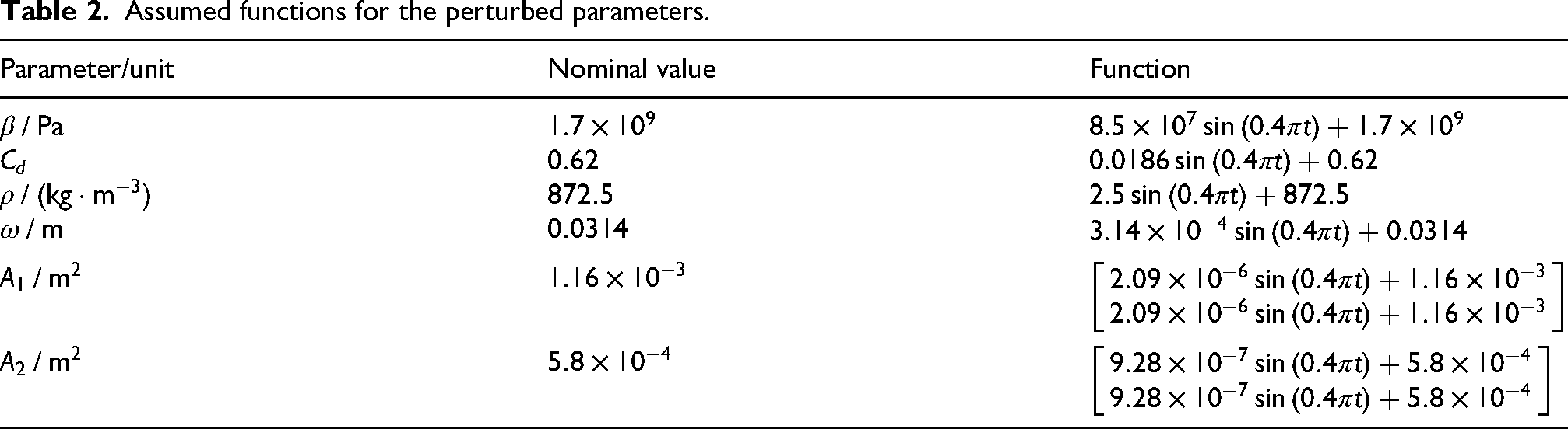
In the simulation, to capture parameter variations under real-world conditions, all system parameters prone to perturbation are assumed to be sinusoidal functions. For example, the spool valve opening $ω$ may experience instantaneous fluctuations due to spool hysteresis, zero drift, and load impact, with a relative perturbation amplitude of $\pm$ 1% to $\pm$ 4%. Given the manipulator's light load in this study, the perturbation is set to $\pm$ 1%. The orifice flow coefficient $C_{d}$ is perturbed by oil temperature fluctuations, instantaneous pressure changes, and flow regime switching. Assuming good hydraulic oil cleanliness and neglecting valve wear, we set its perturbation range to $\pm$ 3%. The bulk modulus $β$ of hydraulic oil, influenced by temperature, pressure, and gas content, decreases with rising system temperature and increases with working pressure. Based on engineering practice, its perturbation amplitude is $\pm$ 5%. The hydraulic cylinder's effective working area depends on cylinder geometric dimensions (e.g. piston diameter and cylinder bore diameter); the cylinder itself is typically made of steel (e.g. carbon steel and alloy steel). Steel's thermal expansion causes slight geometric changes with temperature (60°C–100°C, based on engineering cases), leading to a relative area variation of $\pm$ 0.144% to $\pm$ 0.24%. In this simulation, the relative effective area variation rates of rod and rodless chambers are assumed to be $\pm$ 0.16% and $\pm$ 0.18%, respectively. We list the assumed functions for these perturbed parameters in Table 2.

Table 2.

Assumed functions for the perturbed parameters.

Parameter/unit	Nominal value	Function
$β / Pa$	$1.7 \times 10^{9}$	$8.5 \times 10^{7} \sin (0.4 π t) + 1.7 \times 10^{9}$
$C_{d}$	$0.62$	$0.0186 \sin (0.4 π t) + 0.62$
$ρ / (kg \cdot m^{- 3})$	$872.5$	$2.5 \sin (0.4 π t) + 872.5$
$ω / m$	$0.0314$	$3.14 \times 10^{- 4} \sin (0.4 π t) + 0.0314$
$A_{1} / m^{2}$	$1.16 \times 10^{- 3}$	$[\begin{matrix} 2.09 \times 10^{- 6} \sin (0.4 π t) + 1.16 \times 10^{- 3} \\ 2.09 \times 10^{- 6} \sin (0.4 π t) + 1.16 \times 10^{- 3} \end{matrix}]$
$A_{2} / m^{2}$	$5.8 \times 10^{- 4}$	$[\begin{matrix} 9.28 \times 10^{- 7} \sin (0.4 π t) + 5.8 \times 10^{- 4} \\ 9.28 \times 10^{- 7} \sin (0.4 π t) + 5.8 \times 10^{- 4} \end{matrix}]$

Simulation parameters for controllers are selected as below.

For C2, if ESO is not used to observe system states, the expanded state variable $x_{4}$ cannot be estimated. Thus, the controller can only be designed using nominal values ${\hat{φ}}_{1}, {\hat{φ}}_{2}, and {\hat{φ}}_{3}$ for system parameters. The state variables $x_{2}$ and $x_{3}$ are measured by angular velocity sensors and pressure sensors, respectively. The input vector of the RBF neural network is $x_{n 1} = [x_{1}, x_{2}]^{T}$ , and its hyperparameters are identical to those in C3 (detailed below). The final control law is formulated as:

\begin{aligned} u = \\ {\hat{φ}}_{1}^{- 1} {\begin{matrix} - k_{g} s - ε_{N} \tan (s) + {\hat{φ}}_{2} x_{2} + {\hat{φ}}_{3} + {\dot{x}}_{3 d} - c_{1} {\dot{e}}_{1} \\ - c_{2} {M {(x_{1})}^{- 1} [\begin{matrix} h (x_{1}) x_{3} - C (x_{1}, x_{2}) x_{2} \\ - G (x_{1}) - F (x_{2}) \end{matrix}] - \hat{g} (t) - {\dot{x}}_{2 d}} \end{matrix}} \end{aligned}

As for C3, the input of the RBF neural network in C3 is $x_{n} = [x_{1}, {\hat{x}}_{2}]^{T}$ . In the dual-joint system, since both $x_{1}$ and ${\hat{x}}_{2}$ are two-dimensional vectors, the input layer dimension d of the network is 4. Since it is necessary to predict the external disturbances of the two joints, the output layer dimension of the network is set to 2.

The selection of m, the number of hidden layer nodes in the RBF neural network, needs to simultaneously consider disturbance approximation accuracy, real-time computing efficiency, and system stability. This aims to avoid excessive approximation error caused by an overly small m, as well as overfitting or computational delay caused by an overly large m. In this paper, $m = 11$ is determined through five-fold cross-validation and multidimensional index assessment. It is assumed that the sinusoidal disturbance torques—with directions conforming to the right-hand rule in both tests 1 and 2—are given as:

τ_{d} = [\begin{matrix} τ_{1 d} \\ τ_{2 d} \end{matrix}] = [\begin{matrix} 20 \sin (2 π t) \\ 20 \sin (2 π t) \end{matrix}] N \cdot m

(56)

Firstly, m is determined by the empirical formula $m = 2 d + 1$ ²¹ (where d denotes the input layer dimension) and the initially selected candidate values are 7, 9, 11, 13, and 15. Secondly, 200 sets of data are obtained from simulation experiments. Then, the five-fold cross-validation method is employed. Specifically, these data are randomly and evenly divided into five nonoverlapping subsets. Each time, four subsets are used as the training set to train the model, while the remaining one subset serves as the test set to verify the model's performance. This process is repeated five times to ensure each subset serves as the test set once, and the performance indicators from the five tests are finally averaged as the model's final evaluation result to assess the model's performance in data prediction.

When $m = 7$ , the number of hidden layer nodes is insufficient to capture the nonlinear characteristics of disturbances, and the root mean square error (RMSE) of the test set reaches $0.067$ (joint 1) and $0.064$ (joint 2), respectively. Excessively large approximation errors lead to insufficient compensation of the controller. When $m = 9$ , the approximation capability is improved, and the test set RMSE drops to $0.042$ (joint 1) and $0.040$ (joint 2); however, disturbance approximation lag still emerges under high-speed motion conditions. When $m = 11$ , the test set RMSE further decreases to $0.025$ (joint 1) and $0.022$ (joint 2), and the tracking error stabilizes within 1%, which meets the high-precision control requirements. When $m = 13$ , the test set RMSE only decreases marginally to $0.024$ (joint 1) and $0.020$ (joint 2), representing a mere 9% improvement compared to the results at $m = 11$ . However, the risk of overfitting increases significantly (as evidenced by the training-set RMSE being $0.012$ (joint 1) and $0.009$ (joint 2), widening the gap with the test set), and the robustness decreases under unseen load mutation conditions. When $m = 15$ , the test set RMSE changes minimally to $0.023$ (joint 1) and $0.020$ (joint 2), while the approximation accuracy gap between the training and test sets further widens, that is, the overfitting risk is further exacerbated.

Considering the real-time requirement in this article (control period of 1 $ms$ ), the number of hidden layer nodes needs to match the computational capability of the software. With the aid of MATLAB Profiler, the computation time corresponding to different numbers of hidden layer neurons is quantified. The computation time for different values of m is as follows: when $m = 7$ , the total time consumption per cycle is 620 $μ s$ ; when $m = 9$ , it is 690 $μ s$ ; when $m = 11$ , it is 780 $μ s$ ; and when $m = 13$ , the total time consumption approaches 1000 $μ s$ . It can be seen that when $m = 11$ , the total algorithm consumption is below the 1 $ms$ threshold, allowing more time to be reserved for system communication and I/O delay. Compared with $m = 13$ , it saves nearly 20% of computational resources (with an accuracy improvement of 9%). If the number of nodes is further increased to $m = 15$ , the computational resource cost-effectiveness will decrease further, resulting in severe computational resource redundancy without obvious performance gain, which does not conform to the principle of efficiency. The performance and computation time corresponding to different numbers of hidden layer nodes are shown in Table 3, and their comparison results are illustrated in Figure 5.

Figure 5.

Performance comparison chart of hidden layer node counts.

Table 3.

Performance comparison of hidden layer nodes.

Number of hidden layer nodes	Test set RMSE (joint 1/joint 2)	Training set RMSE (joint 1/joint 2)	Test-training RMSE difference (joint 1/joint 2)	Computation time/unit
$7$	$0.067 / 0.064$	$0.062 / 0.061$	$0.005 / 0.003$	$620 μ s$
$9$	$0.042 / 0.040$	$0.036 / 0.033$	$0.006 / 0.007$	$690 μ s$
$11$	$0.025 / 0.022$	$0.016 / 0.015$	$0.009 / 0.007$	$780 μ s$
$13$	$0.024 / 0.020$	$0.012 / 0.009$	$0.012 / 0.011$	$1000 μ s$
$15$	$0.023 / 0.020$	$0.006 / 0.004$	$0.017 / 0.016$	$1380 μ s$

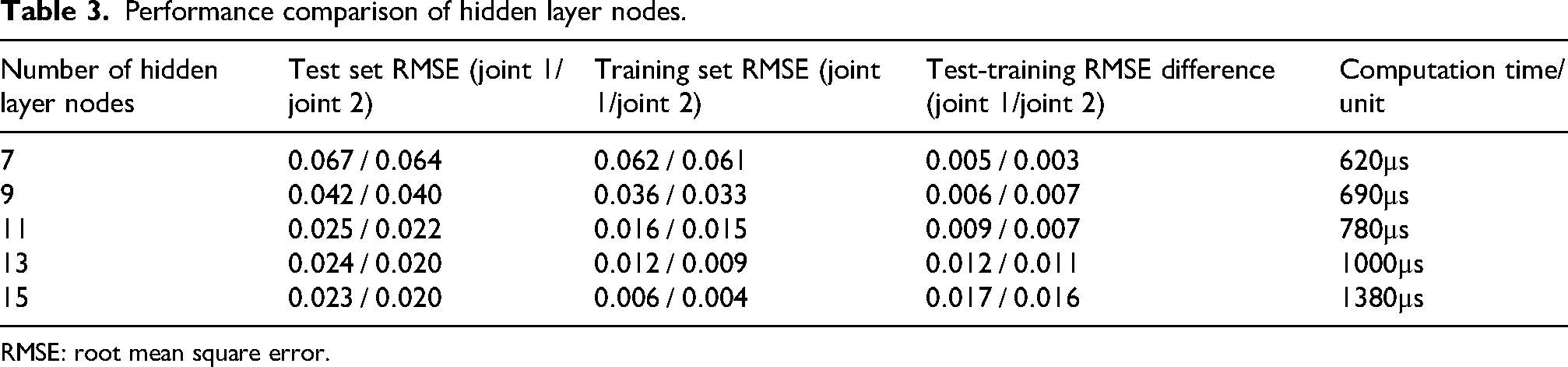
RMSE: root mean square error.

Stability verification: overfitting (excessively large $m$ ) or underfitting (excessively small $m$ ) will cause the approximation model of the RBF neural network for disturbances to deviate significantly from the actual system, thereby triggering oscillations in the control law output and seriously affecting system stability. To verify the stability of the RBF neural network with $m = 11$ hidden layer nodes in the control system, analysis is conducted from two aspects: Lyapunov stability margin and tracking error convergence speed. Firstly, based on the role of the RBF neural network in the system, a Lyapunov function is defined as $V_{r} = \frac{1}{2} e^{T} e + \frac{1}{2} {\tilde{W}}^{T} γ^{- 1} \tilde{W}$ . By differentiating both sides of the equation, we can derive ${\dot{V}}_{r} \leq - k_{r} V_{r} + θ$ , where $k_{r}$ is a positive constant and $θ$ the upper bound of external uncertain disturbances.

When $m = 11$ , we calculate $k_{r} = 0.8 > 0$ and $θ = 0.05$ . According to the Lyapunov exponential stability theorem, this inequality satisfies the exponential stability condition: the system state will evolve toward reducing $V_{r}$ (owing to negative feedback characteristics), enabling exponential convergence to a stable state with disturbance rejection capability. For comparison $m = 13$ , the derivative inequality ${\dot{V}}_{r} \leq - k_{r}^{'} V_{r} + θ^{'}$ still holds, but with $k_{r}^{'} = 0.7$ (smaller than 0.8) and $θ^{'} = 0.08$ (larger than 0.05). A larger $θ^{'}$ value indicates the system is more susceptible to external disturbances, corresponding to a narrower stability margin. This intuitively demonstrates that $m = 11$ exhibits better stability performance in dealing with disturbances and can maintain the stable operation of the system more effectively.

To conclude, based on the aforementioned performance comparison, the number of hidden layer nodes for the RBF neural network is determined as 11, and its structure is 4-11-2.

The kernel width of the neural network is designed using the average distance method, with the design formula: $b_{j} = k_{n} \bar{d}$ .²¹ Here, $k_{n}$ is an empirical coefficient (usually set within the range of 0.5–1.5); $\bar{d} = \frac{1}{m (m - 1)} \sum {‖ c_{i} - c_{j} ‖}_{2}, (i \neq j)$ denotes the average Euclidean distance between all center vectors. Considering the network's input dimension and the number of hidden layer neurons, for low-dimensional input and a moderate number of hidden layer neurons, an empirical coefficient within the intermediate range is more preferable. If the kernel width is excessively narrow, the response of the radial basis function to the input will be overly localized, causing overfitting, whereas an overly large kernel width will lead to poor discriminability of the model and result in underfitting.²² Therefore, $k_{n}$ is taken as an appropriate value of 0.8 here, and through calculation, the width $b_{j} (j = 1, 2, \dots, 11)$ of this network is obtained as 0.42; the initial value of the output layer weight matrix of the network is set as $W = 0.001$ .

After extensive simulation and tuning, the parameters of the ESO are selected as follows: $w_{0} = 120$ , $α_{1} = 2$ , $α_{2} = 1$ , $α_{3} = 1$ , $α_{4} = 0.2$ .

The bandwidth of the ESO $w_{0}$ needs to balance between fast tracking of system states and suppression of sensor noise. According to the standard ESO design criterion, $w_{0}$ should be set to three to five times the bandwidth of the controlled plant to tradeoff between observation speed and disturbance rejection performance. For the 2 degrees of freedom hydraulically manipulator, its inherent response bandwidth (determined by the bulk modulus $β$ , the effective hydraulic area $A$ , and the coupled equivalent load inertia of the two joints) is approximately 30 to 40 Hz. Thus, the theoretical range of $w_{0}$ is derived as $[90, 200]$ Hz. However, simulation results show that when $w_{0} = 105$ Hz, the angular velocity observation exhibits a delay (exceeding the 1 $ms$ control period of the controller) failing to meet real-time requirements. After gradually increasing $w_{0}$ to 120 Hz: no observable delay exists in angular velocity observation; high-frequency noise (amplitude ≤ 0.5% of the signal range) is introduced but remains within the acceptable threshold of the control system. Thus, $w_{0} = 120$ Hz is finally determined.

The characteristic equation of the fourth-order ESO is given by: $s^{4} + α_{1} w_{0} s^{3} + α_{2} w_{0}^{2} s^{2} + α_{3} w_{0}^{3} s + α_{4} w_{0}^{4} = 0$ . To ensure fast convergence, we adopt multiple pole placement and configure all poles as $s = - w_{0}$ (keeping the real parts far from the imaginary axis, avoiding oscillation). Expanding the monic polynomial corresponding to poles $s = - w_{0}$ . The ideal gains are obtained by comparing coefficients: $α_{1} = 4, α_{2} = 6, α_{3} = 4, α_{4} = 1$ .

However, the hydraulic system exhibits strong nonlinearities (e.g. flow-pressure coupling and frictional nonlinearity). Directly applying the ideal gains leads to a 12% overshoot in the observation error. Considering the slight delay in the spool displacement response of the hydraulic servo valve, excessively high $α_{1}$ (first-order gain) and $α_{2}$ (second-order gain) will amplify the delay effect, inducing observation oscillations during startup. Thus, $α_{1}$ is reduced from 4 to 2, and $α_{2}$ is reduced from 6 to 1. After tuning, the overshoot of the observation error is suppressed to $\leq 2 %$ during the system startup phase.

To match the pressure response speed of the hydraulic cylinder and guarantee the observation accuracy of the actuator output force $x_{3}$ , the coefficient associated with the observation bandwidth of $α_{3}$ is reduced from 4 to 1. To avoid observation divergence caused by slight fluctuations in leakage coefficients and inertia parameters, the observation sensitivity of the extended state $x_{4}$ (total parameter perturbation term) is weakened, $α_{4}$ is reduced to 0.2. Through iterative co-simulation of the ESO and the hydraulic manipulator system, the tuned gains $w_{0} = 120$ , $α_{1} = 2$ , $α_{2} = 1$ , $α_{3} = 1$ , $α_{4} = 0.2$ enables effective observation of all system states, and no significant overshoot or oscillation phenomena in the observation process.

To verify the stability of the parameter selection, frequency domain margin analysis and root locus analysis can be employed to ensure the system has no overshoot and no instability risk. The specific results are as below.

Gain margin: 8.2 dB ( $\geq$ 6 dB engineering stability threshold) indicating the system has sufficient tolerance to gain disturbances. Even if the bulk modulus of hydraulic oil decreases by 10% due to temperature changes, stability can still be maintained. Phase margin: 55° ( $\geq$ 45° engineering stability threshold) avoiding resonance caused by phase lag in the hydraulic system. Cutoff frequency: 118 Hz, which matches the observation bandwidth $w_{0} = 120$ Hz (the slight difference prevents high-frequency oscillation induced by bandwidth mismatch).

According to the convergence design criterion of the ESO based on bandwidth, its stability is determined by the pole locations of its error system. The more negative the real part of the pole (i.e. the larger its absolute value), the faster the convergence speed and the more sufficient the stability margin. By plotting the root locus of the ESO's characteristic equation, under the current parameters $w_{0} = 120$ , $α_{1} = 2$ , $α_{2} = 1$ , $α_{3} = 1$ , $α_{4} = 0.2$ , the pole locations are $s_{1} = - 65, s_{2} = - 62, s_{3} = - 58, s_{4} = - 55$ . Among them, the real parts of $s_{1}$ and $s_{2}$ are $\leq - \frac{w_{0}}{2} = - 60$ , satisfying the conservative stability criterion, thus ensuring fast convergence speed and sufficient stability margin. However, the conservative engineering criterion is not a necessary condition for stability: according to control theory, the real part of the pole being negative (located in the left half-plane) is the necessary and sufficient condition for system stability. Thus, even though the real parts of $s_{3}$ and $s_{4}$ are greater than $- 60$ , which does not fully satisfy the conservative design criterion, they still meet the core condition for system stability. This is a tradeoff result between theoretical design and simulation debugging: if the real parts of $s_{3}$ and $s_{4}$ were further reduced (which would require increasing $α_{3}$ and $α_{4}$ ), the ESO's observation sensitivity to nonlinear disturbances in the hydraulic system would be excessively enhanced. This would amplify high-frequency noise in the hydraulic servo valve (e.g. spool flutter) and reduce the system's robustness. Therefore, the current parameters are finally determined through simulation iteration.

The remaining control parameters are selected as $k_{1} = 2.07 \times 10^{7}$ , $k_{2} = 4.18 \times 10^{5}$ , $k_{3} = 1500$ , $c_{1} = 500$ , $c_{2} = 850$ , $k_{g} = 105$ , $ε_{N} = 0.0001$ .

The initial joint angles are given by $q_{o} = (40, 30)^{T} (degree)$ , and the initial angular velocities are ${\dot{q}}_{o} = (0, 0)^{T} (degree / s)$ .The desired joint angular displacements are selected as:

{\begin{matrix} q_{1 d} = 20 \sin (0.4 π t + π) + 40 (degree) \\ q_{2 d} = 15 \sin (0.4 π t) + 30 (degree) \end{matrix}

(57)

Test 1: During the operation of a hydraulic manipulator, joints perform periodic reciprocating motions (e.g. repetitive swings). This leads to periodic variations in inertial, Coriolis, and centrifugal forces, thereby subjecting the joints to periodic dynamic disturbances. To verify the controller's disturbance rejection capability, sinusoidal disturbances (which simulate the aforementioned periodic dynamic disturbances) are adopted, as defined in equation (56).

The tracking results of the three controllers are shown in Figures 6 and 7, and the tracking errors are presented in Figures 8 and 9. As can be observed from the figures, under the conditions of considering joint friction, external disturbances, and hydraulic cylinder leakage. For C1, tracking oscillation occurs during the system startup phase, with the maximum tracking error reaching 1.768° and 1.13°. After 0.68 to 0.7 s, it enters a relatively stable tracking state; however, notable periodic tracking errors ( $\pm$ 0.9°) emerge when the actuator undergoes commutation. For C2, transient oscillation also occurs in the system startup phase, after which the system quickly enters a stable tracking state. Although the chattering throughout the entire process is relatively severe and tracking errors arise during commutation, the overall tracking accuracy is higher than that of C1. In comparison, C3 exhibits the smallest oscillation during the system startup phase and takes the shortest time to achieve steady-state tracking. Moreover, no obvious fluctuations or tracking errors occur during commutation. Both the chattering behavior and tracking accuracy of C3 throughout the entire process are superior to those of C1 and C2.

Figure 6.

Tracking curve of joint 1 (test 1).

Figure 7.

Tracking curve of joint 2 (test 1).

Figure 8.

Tracking error curve of joint 1 (test 1).

Figure 9.

Tracking error curve of joint 2 (test 1).

Figure 10 illustrates the estimation of time-varying disturbances $g (t)$ for the two joints by the RBF neural network. It can be observed that the estimation curves exhibit certain oscillations in the initial period, but then converge rapidly to a stable range. Therefore, the RBF neural network exhibits satisfactory observation performance for the time-varying disturbances in the system.

Figure 10.

Estimation of system disturbances by the radial basis function (RBF) neural network (test 1).

Figures 11 to 13 show the ESO's estimations of the joint angular velocity $x_{2}$ , actuator output force $x_{3}$ , and system extended state variable $x_{4}$ .The tracking results indicate that the ESO achieves satisfactory tracking performance for the system state variables, thereby providing accurate and low-noise state variables for controller design, mitigating the impact of parameter perturbations on the controller, and further enabling feedforward compensation for the control input.

Figure 11.

Observation results of $x_{2}$ by the ESO (Extended State Observer; test 1).

Figure 12.

Observation results of $x_{3}$ by the ESO (Extended State Observer; test 1).

Figure 13.

Observation results of $x_{4}$ by the ESO (Extended State Observer; test 1).

Test 2: To further verify the control performance of the proposed control method, the desired joint angles and initial system state are kept unchanged. During the simulation, uniformly distributed random noise within the range of $[0, 10] N \cdot m$ is applied to both joints throughout the process as a background disturbance; a step disturbance torque (amplitude: 50 $N \cdot m$ ) is simultaneously imposed on both joints from t = 5 s to t = 10 s The tracking performance of the three controllers is then re-evaluated, and their performances are compared.

Figures 14 and 15 present the tracking curves for the two joints. When the external disturbance is replaced with an aperiodic noise signal and a sustained step signa, the tracking performance of the three controllers deteriorates to varying extents relative to test 1—all three schemes exhibit slight chattering.

Figure 14.

Tracking curve of joint 1 (test 2).

Figure 15.

Tracking curve of joint 2 (test 2).

Notably, controller C1 is impacted most severely (with the most pronounced chattering), showing persistent oscillations and nonuniform tracking errors across the entire operation. During the system startup phase, the maximum tracking errors peak at 2.061° (joint 1) and 2.100° (joint 2), accompanied by an oscillation duration of 0.8 to 1 s. Oscillations intensify at actuator commutation instants, leading to further enlarged tracking errors. At t = 5 s, when a step disturbance torque is abruptly applied to both joints, the instantaneous maximum tracking errors surge to 0.94° (joint 1) and 1.32° (joint 2); the settling time required to re-establish a steady state is 0.4 s (joint 1) and 0.2 s (joint 2). In summary, controller C1 demonstrates a limited level of robustness, the poorest tracking accuracy and the longest oscillation duration among the three control schemes.

Controller C2 exhibits superior overall tracking performance compared to C1. Despite a slight lag during the startup phase, it rapidly converges toward the desired angle within 0.3 s, and its oscillation amplitude remains notably smaller than that of C1 across the entire operation. At actuator commutation instants, the tracking error is constrained to a fluctuation range of 0.26° to 0.42° for both joints. Upon application of the step disturbance torque to both joints, the instantaneous tracking errors measure 0.40° (joint 1) and 0.51° (joint 2), with settling times of 0.34 s (joint 1) and 0.17 s (joint 2) required to re-establish steady state. In summary, C2 outperforms C1 in terms of both tracking accuracy and disturbance rejection capacity.

Controller C3 maintains the most robust stability: following system startup, it rapidly locks onto the desired signal, with an exceptionally low oscillation amplitude (0.03°–0.12°) sustained throughout operation. Upon application of the step disturbance torque, the resulting tracking errors are merely 0.11° (joint 1) and 0.24° (joint 2), and the associated settling time is the shortest of the three controllers—joint 1 experiences only negligible oscillation and reverts to steady state almost instantaneously, whereas joint 2 requires 0.16 s to settle. These results indicate that, under aperiodic disturbances, C3 retains the highest control precision and strongest robustness among the evaluated controllers.

Figure 16 presents the approximation results of the RBF neural network for external disturbance torques. From Figure 16, while the neural network does not perfectly capture the exact values of the disturbance torques, it effectively tracks the overall variation trend—thereby mitigating the impact of random noise and step disturbances on tracking performance. However, compared to its performance in test 1, the RBF neural network exhibits limitations in disturbance estimation: it cannot precisely compensate for the effect of disturbances on the joints, which is one of the factors contributing to the degraded tracking accuracy in test 2.

Figure 16.

Estimation of system disturbances by the radial basis function (RBF) neural network (test 2).

Figures 17 to 19 present the observation results of the ESO for the system state variables. From the figures, the ESO still achieves satisfactory observation performance for the system variables, providing accurate and low-noise state variables to support controller design.

Figure 17.

Observation results of $x_{2}$ by the ESO (Extended State Observer; test 2).

Figure 18.

Observation results of $x_{3}$ by the ESO (Extended State Observer; test 2).

Figure 19.

Observation results of $x_{4}$ by the ESO (Extended State Observer; test 2).

To further evaluate the control performance of the three controllers, three metrics are adopted in this article: maximum absolute error (MaxAE), mean absolute error (MAE), and standard deviation of absolute error (SAE), with their expressions given in equations (58) to (60). To eliminate the randomness of single-simulation results and verify that the tracking accuracy improvement of the proposed control method in this article is genuine and effective, 10 independent repeated simulations are conducted for each controller under the two disturbance scenarios (tests 1 and 2). Key conditions (e.g. initial conditions and control signals) are kept identical across all simulations to ensure a fair comparison, while each simulation is run independently to guarantee the statistical independence of the samples. For each controller-joint-performance index ( $MaxAE$ , MAE, and $SAE$ ), 10 corresponding sample values are obtained. Based on these samples, the mean (reflecting typical performance) and standard deviation (reflecting data dispersion) of each index are calculated, and the statistical results are summarized in Table 4. Meanwhile, bar charts with error bars (where error bars represent the standard deviation of 10 repeated simulations) for the two-joint indices of each controller under tests 1 and 2 are plotted, corresponding to Figures 20 and 21, respectively.

MaxAE = max_{k = 1, 2, 3, \dots, n} {| e (k) |}

(58)

MAE = \frac{1}{N} \sum_{k = 1}^{N} | e (k) |

(59)

SAE = \sqrt{\frac{1}{N} \sum_{k = 1}^{N} {(| e (k) | - E_{M})}^{2}}

(60)

Figure 20.

Performance index comparison chart of each controller (test 1).

Figure 21.

Performance index comparison chart of each controller (test 2).

Table 4.

Performance evaluation indices comparison.

Controller	Joint	$MaxAE$ (test 1/test 2)	$MAE$ (test 1/test 2)	$SAE$ (test 1/test 2)
C1	1	$1.768 \pm 0.112$ / $2.061 \pm 0.570$	$0.585 \pm 0.081$ / $1.012 \pm 0.431$	$0.305 \pm 0.066$ / $0.576 \pm 0.292$
C1	2	$1.105 \pm 0.083$ / $2.100 \pm 0.608$	$0.465 \pm 0.067$ / $1.215 \pm 0.517$	$0.231 \pm 0.054$ / $0.628 \pm 0.322$
C2	1	$0.670 \pm 0.084$ / $1.138 \pm 0.366$	$0.080 \pm 0.031$ / $0.349 \pm 0.201$	$0.135 \pm 0.041$ / $0.206 \pm 0.145$
C2	2	$0.817 \pm 0.025$ / $1.256 \pm 0.390$	$0.104 \pm 0.035$ / $0.574 \pm 0.289$	$0.113 \pm 0.038$ / $0.331 \pm 0.168$
C3	1	$0.310 \pm 0.021$ / $0.385 \pm 0.077$	$0.021 \pm 0.007$ / $0.024 \pm 0.009$	$0.029 \pm 0.010$ / $0.035 \pm 0.020$
C3	2	$0.361 \pm 0.035$ / $0.421 \pm 0.097$	$0.026 \pm 0.014$ / $0.030 \pm 0.019$	$0.040 \pm 0.012$ / $0.048 \pm 0.022$

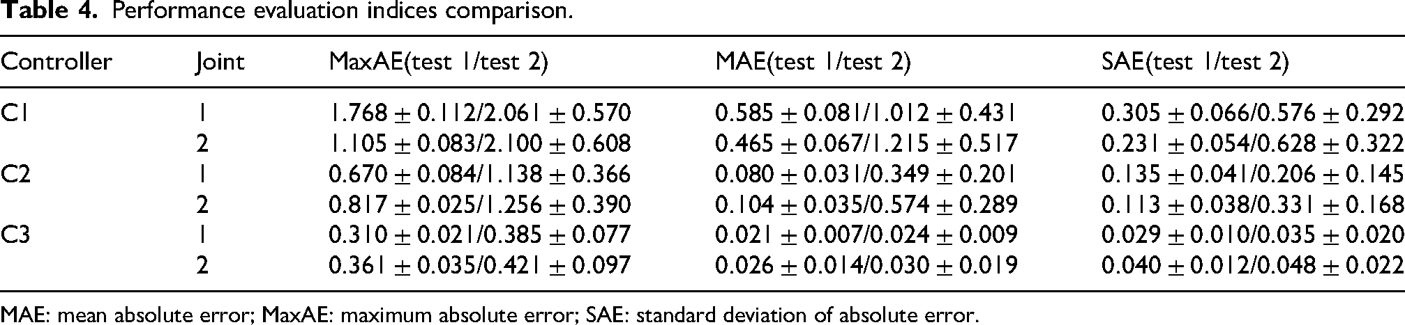
MAE: mean absolute error; MaxAE: maximum absolute error; SAE: standard deviation of absolute error.

For the $MaxAE$ , the control performance of C3 for joint 1 is improved by 82.46% and 53.73% in test 1, 81.34% and 66.16% in test 2 compared to C1 and C2; for joint 2, the improvements are 67.38% and 55.81% in test 1, 79.95% and 66.4% in test 2. Thus, the proposed method achieves a smaller MaxAE, reducing control deviation under extreme conditions and exhibiting superior reliability and safety compared to C1 and C2.

Regarding the MAE, the performance of C3 for joint 1 is improved by 96.41% and 73.75% in test 1, 97.63% and 66.16% in test 2 compared to C1 and C2; for joint 2, the improvements are 94.48% and 75.22% in test 1, 97.53% and 94.77% in test 2. This demonstrates that the smaller MAE of the proposed method indicates lower overall control deviation during long-term operation, thereby enabling the proposed method to achieve the highest long-term accuracy among the three methods.

For the $SAE$ , the control performance of C3 for joint 1 is improved by 90.26% and 78.00% in test 1, 93.92% and 83.01% in test 2 compared to C1 and C2; for joint 2, the improvements are 82.49% and 64.18% in test 1, 92.36% and 85.50% in test 2. Since this metric characterizes error fluctuation, the significant reduction by the proposed method indicates smaller and more stable error fluctuations during operation. This confirms that the method possesses superior consistency and robustness relative to C1 and C2. Overall, comprehensive superior performance in extreme-condition reliability, long-term accuracy, and operational stability.

Analysis of comparative simulation results

As a classic linear controller, C1 generates the control output solely through the proportional (P), integral (I), and derivative (D) terms of the tracking error; essentially, it relies on feedback control based on the “input-output black-box characteristics” and completely ignores the nonlinear coupling characteristics²³(such as dynamic coupling between joints and nonlinear flow-pressure relationship) and time-varying parameter characteristics (such as changes in inertial parameters caused by load variation) of the hydraulic manipulator. Therefore, under the combined effect of periodic disturbances and strong system nonlinearity, C1 is prone to problems including slow response speed, large overshoot, and difficulty in eliminating steady-state errors, with both poor antidisturbance capability and low robustness. These issues are intuitively manifested in the simulation as low trajectory tracking accuracy and obvious fluctuations in the dynamic adjustment process, making it difficult to meet the high-precision trajectory tracking requirements of the hydraulic manipulator.

By leveraging the recursive design concept of backstepping control, C2 gradually stabilizes each subsystem by constructing virtual control laws, and addresses nonlinearities by utilizing the inherent robustness of sliding mode control. Meanwhile, the RBF neural network can approximate the unknown nonlinear components of the system—a capability that theoretically enhances its adaptability to system complexity. However, due to the lack of state observation from the ESO, the system states can only be measured by relying on physical sensors (e.g. angular velocity sensors and pressure sensors). The inevitable measurement noise of sensors will directly corrupt state information, thereby exacerbating the high-frequency chattering of sliding mode control. Furthermore, since the extended state reflecting unmodeled dynamics is unmeasurable, the controller is designed only using the nominal values of system parameters, without considering the time-varying perturbations of leakage and friction coefficients in the hydraulic system, or the dynamic variations of the manipulator's inertial parameters with its posture. When the actual parameters deviate from the nominal values, the approximation error of the neural network and parameter mismatches will jointly lead to a decline in control accuracy. Therefore, although its control performance is significantly improved compared with C1, there still exist chattering phenomena and non-negligible steady-state errors—meaning C2 fails to eliminate chattering or reduce steady-state errors to negligible levels.

Based on the control framework of C2, C3 incorporates an ESO to estimate system states and total parameter perturbations in real time. On the one hand, the observed states provided by the ESO can replace sensor measurements that are susceptible to noise corruption, supplying cleaner and more accurate feedback information for the recursive design of BSMC, thus suppressing noise-induced chattering at the root. On the other hand, the ESO's estimation of parameter perturbations can be directly incorporated into the control law through feedforward compensation, thereby proactively counteracting the impact of parameter perturbations and external disturbances on the system. These two improvements enable the controller to achieve fast response speed, small overshoot, and high-precision trajectory tracking even under complex operating conditions—in which a precise mathematical model is unknown, sensor noise exists, and parameters are time-varying.

Compared with test 1, the tracking accuracy of test 2 decreases to a certain extent. The reasons for this phenomenon are analyzed from two perspectives: physical characteristics and control theory, as below.

Periodic sinusoidal disturbances in real scenarios mainly stem from periodic load variations—such as inertial load fluctuations when the manipulator repeatedly executes the same trajectory, pump pressure pulsations, and the periodicity of joint friction. These disturbances are characterized by fixed frequency and predictable amplitude. By contrast, random noise has more complex and irregular sources, including sensor measurement noise, turbulent noise of hydraulic fluid (caused by the irregular flow of high-pressure oil at valve ports and in pipes), and external random disturbances (e.g. collisions in the working environment and sudden load changes). Such noise is defined by aperiodicity and randomness.

The hydraulic system inherently exhibits characteristics like nonlinear dead zone, fluid compressibility, and frictional nonlinearity. These properties interact with different disturbances to produce a superposition effect, which is further amplified under random noise. This serves as one of the core physical inducements for the degraded tracking accuracy. When confronting periodic disturbances, the system's nonlinearity enables the formation of a stable disturbance-response mapping via the regularity of the disturbances. However, for random noise, its irregularity continuously disrupts this stable mapping; when combined with the hydraulic system's nonlinearity, this leads to issues including joint chattering, increased instantaneous errors, and fluctuations in steady-state errors.

From the perspective of control theory and the practical performance of the RBF neural network: its core advantage lies in high-precision approximation of continuous, smooth, and regular nonlinear functions, but it faces distinct constraints in real applications. Since the input–output mapping of disturbance signals is repetitive and regular, the RBF network converges to stable approximation accuracy after only a small number of iterations. In contrast, the input–output mapping of random noise lacks any regularity—fully approximating it would require an infinite number of radial basis nodes, which is engineering-impractical. In real-time control, the RBF's weight update speed (based on the gradient descent method) cannot match the instantaneous changes of noise; additionally, the high-frequency components of noise exceed the RBF's approximation bandwidth, resulting in unavoidable estimation errors. Thus, the RBF network cannot accurately estimate random noise. The resulting estimation errors lead to an insufficient compensation term, so uncompensated noise acts directly on the joints, causing the decline in tracking accuracy.

Discussion on the computational complexity and real-time feasibility

The computational complexity of the proposed composite control strategy is determined by three core modules: RBF neural network, fourth-order linear ESO, and BSMC, and it is overall at a low level feasible for industrial applications. The RBF neural network adopts a 4-11-2 structure, with computations including forward propagation (involving 4-11 input-hidden layer weight multiplications, 11 Gaussian activation function calculations, and 11-2 hidden-output layer weight multiplications) and weight update (based on gradient descent adaptive law, requiring outer product calculation of 2-dimensional output error vector and 11-dimensional hidden layer activation output vector, plus weight correction with learning rate). The total operations of the RBF module are only several hundred per control cycle. The fourth-order linear ESO relies on fixed-structure linear matrix operations for state prediction and update, involving only basic arithmetic operations without additional overhead, despite its order-related computation volume. The BSMC is derived from the system model, observer output, and RBF approximation results, with computations limited to algebraic operations and sliding surface derivative solution, which leads to no significant increase in computational complexity.

Mainstream standard industrial hardware (e.g. Intel Core i5/i7 industrial computers, STM32H7 series embedded controllers) generally has a single-core clock frequency of 1 to 2 GHz, with each basic arithmetic operation taking only 1 to 2 ns. Even with a conservative estimate—1000 basic arithmetic operations plus 50 complex operations such as activation function/gradient calculation—the total theoretical time consumption of the proposed algorithm is only 50 to 100 ns. This is far below the 1ms target, leaving sufficient time margin to cope with additional overheads like system communication and I/O delays. Thus, the algorithm has low overall computational load and theoretically meets the real-time requirements of industrial hardware.

However, the algorithm has the potential limitations: For 6-DOF robotic arms, the input dimension of the RBF increases to 12, leading to higher computational latency, which necessitates subsequent model order reduction or hardware acceleration.

In future work, we will establish a physical platform for a two-joint hydraulic manipulator, validate the performance of the proposed strategy under actual working conditions, and explore the control optimization of a 6-DOF manipulator based on model order reduction.

Conclusion

In summary, this article proposes a composite control strategy that integrates the ESO, RBF neural network, and BSMC. Through the mutual complementarity among these modules, it effectively overcomes the limitations of traditional control methods (i.e. insufficient accuracy and weak robustness) in scenarios with unknown models and multisource disturbances. Based on extensive simulations, the following conclusions are drawn:

ESO effectively achieves accurate observation of system states, thus providing accurate, low-noise state information for controller design. Furthermore, by reconstructing the system model and enabling state observation of parameter perturbations, the ESO directly provides feedforward compensation for the servo valve's control input—significantly enhancing the control precision of the servo valve and laying a foundation for the overall system's stability.

The RBF neural network effectively updates network weights through online learning, which enables accurate estimation of time-varying disturbances. This delivers reliable disturbance information to the controller's disturbance compensation module, effectively suppressing the adverse impacts of time-varying disturbances on system performance and complementing the ESO's capability in handling unmodeled dynamics.

For the hydraulically driven manipulator system, the proposed control strategy exhibits higher control accuracy and stronger robustness compared with PID control and the traditional neural network-based BSMC. This advantage is particularly prominent under complex operating conditions (e.g. unknown precise mathematical models, sensor noise, and parameter perturbations), as the synergistic integration of ESO's state observation, RBF's disturbance estimation, and BSMC's nonlinear regulation enables the strategy to address multisource uncertainties comprehensively.

Footnotes

Acknowledgements

Thanks to the School of Mechanical Engineering of Shenyang University of Technology for the support to this study. Thank you for the help of my peers in the research. Finally, thank the reviewers and editors for their valuable comments, so that the content of the article more complete.

ORCID iD

Feihong Liu

Funding

The authors received no financial support for the research, authorship, and/or publication of this article.

Declaration of conflicting interests

The authors declared no potential conflicts of interest with respect to the research, authorship, and/or publication of this article.

References

Wei

, et al. Adaptive dynamic programming-based cross-scale control of a hydraulic-driven flexible robotic manipulator. Appl Sci-Basel 2023; 13: 27.

Cardoso

Schnitman

. Analysis of exact linearization and approximate feedback linearization techniques. Math Probl Eng 2011; 2011: 17. Art. no. 205939.

Jiang

Tao

, et al. A direct adaptive actuator failure compensation scheme for satellite attitude control systems. Proc Inst Mech Eng G-J Aerosp Eng 2014; 228: 542–556.

. Comments on ‘A new terminal sliding mode control for robotic manipulators’. Int J Control 2017; 90: 247–254.

Liu

Chai

Sun

, et al. An adaptive iterative learning control approach based on disturbance estimation for manipulator system. Int J Adv Rob Syst2019; 16: 13. Art. no. 1729881419852197.

Zhu

Zhong

. Editorial: hybrid intelligent algorithms based learning, optimization, and application to autonomic control systems, volume II. Front Neurorobot 2023; 17: 3. Art. no. 1151473.

Yang

Wei

, et al. Non-recursive fixed-time convergence observer and extended state observer. IEEE Access 2018; 6: 62339–62351.

Razmjooei

Palli

Abdi

, et al. Finite-time continuous extended state observers: design and experimental validation on electro-hydraulic systems. Mechatronics (Oxf) 2022; 85: 17. Art. no. 102812.

Guo

. Extended-state-observer based sliding mode control for pump-controlled electro-hydraulic servo system. J Beijing Univ Aeronaut Astronaut 2020; 46: 12.

10.

Chen

, et al. Practical finite-time observer-based adaptive backstepping super-twisting sliding mode control for deep-sea hydraulic manipulator. IEEE Trans Ind Electron 2025; 2025: 11.

11.

Donas

Kordatos

Alexandridis

, et al. A dual filter based on radial basis function neural networks and Kalman filters with application to numerical wave prediction models. Sensors 024; 24: 24. Art. no. 8006.

12.

Zhang

Duan

. Adaptive event-triggered output feedback consensus tracking control of multi-agent systems via K-filters. Int J Robust Nonlinear Control 2025; 35: 2354–2366.

13.

Wang

Cao

, et al. An improved pelican optimization-kernel extreme learning machine for highly accurate state of charge estimation of lithium-ion batteries in energy storage systems. Ionics 2025; 31: 5809–5825.

14.

Feng

Zhang

Tian

. Integrated sliding mode control of robot manipulator based on fuzzy adaptive RBF. J Northwestern Polytech Univ 2024; 42: 1746–1759.

15.

Zhao

Zhang

, et al. Disturbance observer-based neural network control of a 2-DOF helicopter system with input saturation and output constraints. IEEE Trans Syst Man Cybern-Syst 2025; 55: 3152–3162.

16.

Ding

. Model-based control of the hydraulic manipulator for the high-precision trajectory tracking. J Mech Eng 2023; 59: 298–309.

17.

Guo

Tateno

. Semantic web-driven hybrid adaptive control system for trajectory tracking in robotic arms. Int J Semantic Web Inf Syst 2025; 21: 1–30.

18.

Peng

Jayawardhana

Xin

. Distributed end-effector formation control for networked 2-DoF flexible-joint manipulators with partially underactuated agents. Automatica (Oxf) 2025; 179: 13. Art. no. 112453.

19.

Yang

Kun

Shuang

, et al. Study on static and dynamic characteristics of the electro-hydraulic proportional directional valve. Proc Instit Mech Eng C-J Mech Eng Sci 2025; 2025: 18.

20.

Wang

. An iterative tuning method for feedforward control of parallel manipulators considering nonlinear dynamics. Chin J Mech Eng 2025; 38: 11. Art. no. 19.

21.

Czarnowski

Jedrzejowicz

. Designing RBF networks using the agent-based population learning algorithm. New Gener Comput 2014; 32: 331–351.

22.

Rafajlowicz

Pawlak

. Optimization of centers’ positions for RBF nets with generalized kernels. In: Rutkowski

Siekmann

Tadeusiewicz

Zadeh

(eds) Artificial intelligence and soft computing - Icaisc 2004. (Lecture Notes in Artificial Intelligence), 3070. Berlin: Springer-Verlag Berlin, 2004, pp.253–259.

23.

Fan

Gao

. Fuzzy neural network PID control design of Camellia fruit vibration picking manipulator. J Agri Eng 2023; 54: 12.

Research on neural network-based composite control strategy for hydraulically driven manipulators

Abstract

Keywords

Introduction

System description

Controller design

Analysis of the simulation process and comparison of result

Simulation process

Analysis of comparative simulation results

Discussion on the computational complexity and real-time feasibility

Conclusion

Footnotes

Acknowledgements

ORCID iD

Funding

Declaration of conflicting interests

References