A backbone-based inverse kinematics and head traction path-following algorithm for soft manipulators

Abstract

This paper introduces an inverse kinematics solution and a path-following method for a tendon-driven soft manipulator. The inverse kinematics problem is addressed using a modified backbone method, where the spatial backbone is defined by the modal function to accommodate various mission requirements. With this novel approach, a soft manipulator comprising three constant curvature segments can be accurately fitted to a designated multi-curvature backbone. Notably, the method eliminates the need to select a backbone curve with identical curvature to that of the manipulator, enabling the use of a specific backbone to solve the inverse kinematics for soft manipulators with diverse configurations. Consequently, the solution can be swiftly and accurately computed within the workspace. Furthermore, drawing inspiration from snake locomotion, a “head traction” path-following algorithm is proposed in conjunction with the modified backbone inverse kinematics. This algorithm facilitates the manipulator's maneuvering along with a predefined path in complex environments, avoiding collisions with obstacles. Finally, the feasibility of both algorithms is validated through comprehensive simulations.

Introduction

In the past decade, soft manipulators research has been a popular thesis in the field of manipulators, ¹ mainly because of their ability to adapt to the complex environment, ² more flexible choice of materials, ³ and allowing humans to interact with the environment more securely. ⁴ These manipulators can be applied in areas where traditional rigid manipulators cannot be used, such as medical endoscopes and wearable technology. ⁵

In space acquisition missions, soft manipulators also have a wider range of application than traditional rigid manipulators on account of their fine environmental compliance.^6–8 Compared with the rigid manipulator, soft manipulators with multi-arm segments can enter a more complex environment to perform spacecraft detection and capture tasks.^9–11 In addition, the drive part of the soft manipulator can be put inside a spacecraft, which can improve security and reduce the costs of space missions.

Soft manipulators are typically categorized into pneumatic-based^12,13 and tendon-driven types based on their actuation mechanisms.^14,15 Due to the limitations of air sources, tendon-driven arms are used more widely than pneumatic-based arms. Those manipulators have some unique characteristics such as high nonlinearity and hyper-redundancy, which make their kinematic control different from traditional rigid manipulators. The kinematic modeling approach of soft manipulators includes model-based controllers and model-free controllers. ¹⁶ Both methods describe the kinematics characteristics according to the drive parameters of the manipulator. The model-free approach does not need a physical manipulator model. It uses mostly machine learning, and it can solve the soft manipulator's forward and inverse kinematics. The model-free approach has recently emerged as a significant research area. Lee et al. proposed a general control framework based on nonparametric local framework training to directly learn the inverse model of a soft manipulator. ¹⁷ This method does not require prior knowledge of manipulator's structural parameters and it has achieved high-precision navigation and control in the field of endoscopy. Melingui et al. proposed an approach using remote supervised learning and an adaptive neural network to control the end effector position of a manipulator namely Compact Bionic Handling Assistant (CBHA). ¹⁸ Also for a CBHA manipulator, Rolf and Steil used a babbling-based online simulation learning method, which is a combination of machine learning and traditional feedback control. ⁶ The authors performed a substantial experimental verification of this method. For soft manipulators with nonunique curvature, Giorelli et al. introduced a supervised learning method and designed an experiment combining this algorithm with feed-forward neural networks. ¹⁹ Verification experiments demonstrated that the model-free method can control a nonunique curvature manipulator with high precision.

For a soft manipulator with unique curvature, the model-based method is relatively mature. The most common model-based method is the constant curvature method.^20,21 Gravagne and Walker had proposed constant curvature kinematics model earlier and used it to solve the maneuverability and compliance of a soft manipulator. ²² This method is a good approximation of the static problem of soft manipulators, ¹⁶ but it also has some limitations. For instance, it is only applicable to manipulators with a symmetric structure and external loads. Moreover, the approach can only be truly effective under steady-state conditions. In addition, for unique curvature manipulators, the kinematics can also be solved by the relevant beam theory. ²³ Gao et al. offered a fixed guide beam theory to predict symmetrical constant curvature manipulators accurately. The shape of the manipulator could be deformed and good experimental results were obtained. ²⁴ Renda et al. proposed a Cosserat-based beam theory to solve the kinematics and dynamics of a soft manipulator. ²⁵

After the forward kinematics model has been established, the model needs to be solved reversely. The inverse kinematics issue has not been solved comprehensively. Bailly et al. introduced numeral calculation approaches, which derived the inverse kinematic models from the forward kinematics model.^26,27 Although the calculation process is complex, the forward kinematic model cannot repeatedly obtain accurate analytical solutions.^28,29 Mu et al. established a relationship between the shape of a hyper-redundant planar manipulator and its actuators by using a segment geometry-based method. ³⁰ Singh et al. led to a Pythagorean hodograph method to solve the inverse kinematics of soft manipulators. ³¹ In recent years, many methods that use machine learning to perform inversion of soft manipulator kinematics have been developed. ³² In principle, the kinematic inversion of any manipulator can be calculated by these methods. However, in actual use, small environmental disturbances may cause large solution errors. ¹⁶

The main contribution of this work is an approach to efficiently and accurately solve the inverse kinematics of multisegment, unique-curvature soft manipulators. Furthermore, based on the backbone-based inverse kinematics algorithm, a path-following algorithm is proposed, enabling the soft manipulator to navigate complex environments while avoiding collisions with obstacles. A soft manipulator with less-quantity constant curvature segments, for example, manipulator with three constant curvature segments which is the common configuration of soft robot, can be fitted to the defined backbone regardless of the backbone curvature amount. The core of this method is considering the case where the curvature of the soft manipulator does not match the curvature of the backbone, to make the inverse kinematics algorithm for soft manipulators more versatile. The improved method does not need to identify a backbone with exactly the same curvature as the soft manipulator, which can reduce the complexity of the inverse kinematics-solving process. In the path-following algorithm, the configuration parameters of the latter arm segment are always the same as those of the previous segment, only two kinematic parameters need to be solved, which can greatly simplify the path-fitting process.

The remainder of this paper is organized as follows: “Soft manipulator and kinematics model” section introduces the kinematic model of a tendon-driven soft manipulator with three segments. In “Backbone-based inverse kinematics solution” section, a method using the improved backbone method combined with the kinematic model is proposed to solve the inverse kinematics of the soft manipulator. “A head traction path-following algorithm” section suggests a path-following algorithm. “Simulation and experiment” section submits the simulation results and experiment of the proposed inverse kinematics method and path following the control method. The final section summarizes the whole paper and gives the conclusion.

Soft manipulator and kinematics model

Design of the soft manipulator

This Study Introduces a novel soft manipulator design that significantly differs from the conventional rigid articulated arms. Notably, the driving motors are concentrated at one end of the arm, and the driving force is transmitted through cables, as shown in Figure 1. The soft manipulator is composed of three segments, each driven by four circumferentially arranged tendons. The four tendons in each segment are evenly spaced at 90° intervals around the circumference, while tendons in adjacent segments are arranged at 90° clockwise intervals. In this configuration, six motors drive 12 wires, compensating for minor length discrepancies between two wires sharing a single motor through motion compensation, a technique that has demonstrated practical effectiveness.^3334–35

Figure 1.

Schematic diagram of a soft manipulator.

Manipulator kinematics model

In the kinematics model of soft manipulator, the arm segment can be regarded as n (which is the same as the number of arm segments) arcs with different curvature angles and different bending planes. The i-th segment arc can be described by three parameters, namely curvature $k_i$ , deflection angle ${\varphi }_i$ , and arc length $s_i$ .

As shown in Figure 2, there is one manipulator segment in the kinematics model, in which $l_{i1}$ , $l_{i2}$ , $l_{i3}$ , and $l_{i4}$ represent four driving tendons, and coordinate system $o_i$ is established on i-th segment of the arm. The origin of the system is placed at the center of i-th segment, the x-axis of the coordinate system points to the driving-tendon $l_{i1}$ , the y-axis of the coordinate system points to driving-tendon $l_{i2}$ , and the z-axis of the coordinate system is determined by the right-hand rule.

Figure 2.

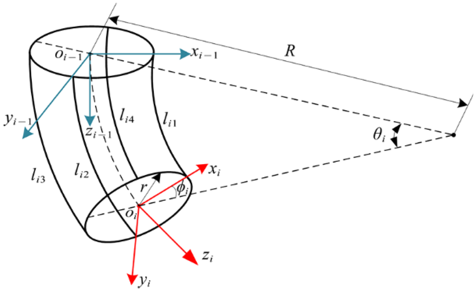
Schematic diagram of the mechanical arm segment in the kinematic model.

In Figure 2, the plane indicated by the broken line is a defined deflection plane, and deflection angle ${\varphi }_i$ is defined as the angle between the plane and the positive direction of the coordinate system x-axis. Curvature bending angle ${\theta }_i$ is defined as shown in Figure 2. Arc $\stackrel{\cap }{o_{i-1}{o}_i}$ represents the centerline of the arm, r represents the radius of the arm segment, and R represents the curvature radius of the arm segment bend.

The kinematic model of the soft manipulator is developed under some assumptions, described below:

The manipulator segment is regarded as a rigid body, and internal elastic deformation is not considered during the movement. In the initial movement, lengths of the respective driving tendons are equal to the length of the manipulator centerline.

The frictional influence of driving-tendons is not considered when moving in via hole, and it is assumed that the driving-tendon does not have tensile deformation.

During the movement of an arm segment, the attitude of the arm is ignored, and only the relative position of the end effector is considered.

Under those assumptions, the motion change at the end of the manipulator can be seen as a process of transforming from coordinate system $o_{i-1}$ to coordinate system $o_i$ :

Coordinate system $o_{i-1}$ rotates ${\varphi }_i$ around the z-axis;

Coordinate system $o_{i-1}$ rotates $\frac{{\theta }_i}{2}$ around the transformed y-axis;

Coordinate system $o_{i-1}$ moves along with line $o_{i-1}{o}_i$ for a distance of $|o_{i-1}{o}_i|$ ;

Coordinate system $o_{i-1}$ rotates $-\frac{{\theta }_i}{2}$ around the transformed y-axis;

Coordinate system $o_{i-1}$ rotates $-{\varphi }_i$ around the transformed z-axis.

The coordinate transformation process, combined with the geometric relationship of arm parameters yields a transformation matrix from coordinate system $o_{i-1}$ to coordinate system $o_i$ of the manipulator segment, is given by

$${}_{i-1}^{i}T=\left[\begin{array}{c}{\mathit{R}}_{i-1}^i\\ 0\end{array}\begin{array}{c}{\mathit{P}}_{i-1}^i\\ 1\end{array}\right]$$

(1)

where ${\mathit{R}}_{i-1}^i$ can be given by

$${\mathit{R}}_{i-1}^i=\left[\begin{array}{c}{c}^2{\varphi }_i(c{\theta }_i-1)+1\\ s{\varphi }_{i}c{\varphi }_i(c{\theta }_i-1)\\ -c{\varphi }_{i}s{\theta }_i\end{array}\begin{array}{c}s{\varphi }_{i}c{\varphi }_i(c{\theta }_i-1)\\ s^2{\varphi }_i(c{\theta }_i-1)+1\\ -s{\varphi }_{i}s{\theta }_i\end{array}\begin{array}{c}c{\varphi }_{i}s{\theta }_i\\ s{\varphi }_{i}s{\theta }_i\\ c{\theta }_i\end{array}\right]$$

(2)

and ${\mathit{P}}_{i-1}^i$ can be given by

$${\mathit{P}}_{i-1}^i=\left[\begin{array}{c}||o(s)||\cdot c{\varphi }_i(1-c{\theta }_i)\\ ||o(s)||\cdot s{\varphi }_i(1-c{\theta }_i)\\ ||o(s)||\cdot s{\theta }_i\end{array}\right],$$

(3)

where $s(\cdot )$ represents the function $\sin (\cdot )$ , $c(\cdot )$ represents the function $\cos (\cdot )$ , $\Vert o(s)\Vert =\frac{2s}{{\theta }_i}\sin ({\theta }_i)$ , and s represents the length of a single segment of the arm.

Figure 3 illustrates the arm structure described in this paper. According to the kinematics “chain rule,” its kinematic model can be written as follows:

$${}_0^{3}T{=}_0^{1}T{\cdot }_1^{2}T{\cdot }_2^{3}T.$$

(4)

Figure 3.

Manipulator kinematics model diagram.

It is necessary to determine the mapping relationship between joint space and operating space of the mechanical arm after the kinematics model has been established. Considering tendon layout over the entire manipulator, combined with the geometric relationships illustrated in Figure 2, and based on the constant curvature assumption, a mapping between the tendon's length and manipulator's drive parameters can be derived as follows:

$$\{\begin{array}{c}{l}_{i1}={\theta }_i*l+\sum _{i=1}^3-r{\theta }_i\cos \left({\varphi }_i+(i-1){\displaystyle \frac{\pi }{6}}\right)\\ l_{i2}={\theta }_i*l-\sum _{i=1}^{3}r{\theta }_i\sin \left({\varphi }_i+(i-1){\displaystyle \frac{\pi }{6}}\right)\\ l_{i3}={\theta }_i*l-\sum _{i=1}^{3}r{\theta }_i\cos \left({\varphi }_i+(i-1){\displaystyle \frac{\pi }{6}}\right)\\ l_{i4}={\theta }_i*l+\sum _{i=1}^3-r{\theta }_i\sin \left({\varphi }_i+(i-1){\displaystyle \frac{\pi }{6}}\right)\end{array}$$

(5)

where $l_{ij}$ is the length of the j-th driving-tendon in the i-th arm segment. l is the length of the manipulator's centerline.

According to (3), solution ${\varphi }_i$ is generally not unique. In the actual simulation experiment, when $\mathrm{\Delta }{l}_1\ge 0,\mathrm{\Delta }{l}_2<0$ , ${\varphi }_i\in \left[0,\frac{\pi }{2}\right]$ ; when $\mathrm{\Delta }{l}_1\ge 0,\mathrm{\Delta }{l}_2\ge 0$ , ${\varphi }_i\in \left[\frac{\pi }{2},\pi \right]$ ; when $\mathrm{\Delta }{l}_1<0,\mathrm{\Delta }{l}_2<0$ , ${\varphi }_i\in \left[\pi ,\frac{3\pi }{2}\right]$ ; and when $\mathrm{\Delta }{l}_1<0,\mathrm{\Delta }{l}_2\ge 0,{\varphi }_i\in \left[\frac{3\pi }{2},2\pi \right]$ .

Backbone-based inverse kinematics solution

Modal backbone curve

The modal function backbone method was first proposed and used on a super-redundant rigid manipulator by Chirikjian and Burdick. ³⁶ The parameter expression for the backbone can be written as the form of expression:

$$X(s)=\underset{0}{\overset{s}{\int }}L\mathrm{u}(\sigma )d\sigma$$

(6)

where $s\in [0,1]$ is the length parameter of the curve, $u(\sigma )$ is the unit tangent vector of the curve at $\sigma$ , and L is the length of the curve.

Equation (6) can be extended to obtain:

$$\mathit{X}(s)=\left[\begin{array}{c}\underset{0}{\overset{s}{\int }}L\sin K(\sigma )\cos T(\sigma )d\sigma \\ \underset{0}{\overset{s}{\int }}L\cos K(\sigma )\cos T(\sigma )d\sigma \\ \underset{0}{\overset{s}{\int }}L\sin T(\sigma )d\sigma \end{array}\right],$$

(7)

where $K(\sigma )$ and $T(\sigma )$ are expressed as linear combinations of linearly independent basis functions, as follows:

$$\begin{array}{c}K(\sigma )=\sum _{i=1}^{n_1}{a}_i{f}_i(s)+\sum _{i=1}^2{b}_{i\varphi }{g}_i(s)\mu (\sigma )\\ T(\sigma )=\sum _{i=n_1+1}^{n_2}{a}_i{f}_i(s)+\sum _{i=1}^2{b}_{i\psi }{g}_i(s),\end{array}$$

(8)

here $\{f_i(s)\}$ is the selected modal shape function, $n_1$ is the number of modal shapes $K(\sigma )$ , $n_2$ is the total number of modal shapes $\mu (\sigma )$ , $\{g_i(s)\}$ , and $\{b_{i\phi },b_{i\mu }\}$ are used to specify the orientation of the backbone curve, and $a_i$ is the coefficient of the modal function, which determines the shape of the entire curve. In which, $K(\sigma )=$ $a_1\sin (2\pi \sigma )+a_2(1-\cos (2\pi \sigma ))$ , $\mu (\sigma )=a_3(1-\cos (2\pi \sigma ))$ $\sigma \in [0,1]$ . The $a_i$ is determined by iterative calculation.

Modified backbone inverse kinematics

In practice, a space inverse kinematic backbone or path often comprises a complex multi-curvature, multi-torsion spatial curve. However, the implementation of a multi-curvature backbone in an actual soft manipulator poses challenges. Typically, existing soft manipulator arms is designed with no more than 10 mechanical arm segments, ³⁷ while many referenced soft manipulators feature no more than three arm segments, thereby restricting the adaptable path curvatures. Given this context, this paper introduces the “virtual path point” method for addressing the inverse kinematics of a soft manipulator.

The comparison and conceptual illustration is presented in Figure 4. Figure 4(a) shows the determined spatial backbone curve with 10 different curvatures. Figure 4(b) shows the traditional backbone fitting method,^36,38,39 which must find a backbone curve similar to the n-segments soft manipulators. When the manipulator only has three arm segments just like the arm in this research, which is the most common structure type of the soft manipulator, it is difficult to determine a matching spatial backbone curve. Obviously, when the number of soft manipulator segments is changed, the backbone must be redefined.

Figure 4.

Spatial backbone diagram.

Figure 4(c) shows the modified fitting method. The red thick line represents the fitted arm segments, while the reddish-brown dotted line indicates an alternative posture of the manipulator segments. The manipulator is designed with only three segments, each with distinct curvature, so the backbone does not need to be redefined. This method increases the tolerance of the backbone configuration for soft manipulators.

First, the backbone curve is determined based on the position of the end-effector. Since the backbone curve is a multi-curvature curve, and the curvature of the soft manipulator is limited, the “virtual path point” method is employed to address the “curvature singularity” issue for a manipulator with three constant curvature segments.

The modified method has the following two aspects of improvement:

A three-segment soft manipulator adapts to a multi-curvature backbone curve. This approach avoids the need to select a backbone curve with identical curvature to that of the manipulator, thereby reducing computational complexity.

By selecting different “virtual path points,” the manipulator can achieve various postures at the same end-effector position.

As shown in Figure 5, the black thin line represents the determined spatial backbone, and the red thick line indicates the fitted arm. During the fitting process, the first and last node positions of an arm segment are determined as follows:

$$|p_{\mathit{i}1}{p}_{\mathit{i}3}|=2\times {\displaystyle \frac{S}{\theta }\sin {\displaystyle \frac{\theta }{2},}}$$

(9)

where S represents the length of a single segment of the arm and $\theta$ represents the motion curvature angle of the manipulator, $\theta \in [-\pi /2,\pi /2]$ . Furthermore, $|p_{\mathit{i}1}{p}_{\mathit{i}3}|\in [0.9S,S]$ can be found, where $p_{ij}$ represent the j-th node of the i-th arm.

Figure 5.

Schematic diagram of arm segment fitting.

To ensure that each segment of the mechanical arm is accurately fitted to the specified path, the vector pointing from the end of the arm and the tangent vector of the path are calculated. An appropriate angle is chosen to minimize deviation errors during fitting and to determine the direction vector of the end effector.

The backbone vector for each point is

$$\mathit{s}=\left[\begin{array}{c}\sin \phi (\sigma )\cos \mu (\sigma )\\ \cos \phi (\sigma )\cos \mu (\sigma )\\ \sin \mu (\sigma )\end{array}\right],$$

(10)

where $\phi (\sigma )$ and $\mu (\sigma )$ are combinations of nonlinearly related mode functions.

The fitting of the arm segment, because of its constant curvature, can be expressed by the following functions:

$$\{\begin{array}{c}x=C_x+R(\widetilde{u_x}\cos \theta +\widetilde{v_x}\sin \theta )\\ y=C_y+R(\widetilde{u_y}\cos \theta +\widetilde{v_y}\sin \theta )\\ z=C_z+R(\widetilde{u_z}\cos \theta +\widetilde{v_z}\sin \theta )\end{array}$$

(11)

where $u=[u_x,u_y,u_z{]}^T$ is a vector of the plane of the arm segment, $n=[n_x,n_y,n_z{]}^T$ is the normal vector of the plane of the arm segment, $v=n\times u$ , and $\tilde{u}=[{\tilde{u}}_x,{\tilde{u}}_y,{\tilde{u}}_z{]}^T$ and $\tilde{v}=[{\tilde{v}}_x,{\tilde{v}}_y,{\tilde{v}}_z{]}^T$ are the unit vectors of vectors $\mathit{u}$ and $\mathit{v}$ . Angle $\theta$ is the angle of curvature of the arm. $[C_x,C_y,C_z]$ is the center coordinates in the global coordinate system, and it can be solved in algorithm 1.

Thus, the tangent vector of the arm segment at any point can be expressed as follows:

$$\mathit{a}=\left[\begin{array}{c}{\displaystyle \frac{dx}{d\theta }}\\ {\displaystyle \frac{dy}{d\theta }}\\ {\displaystyle \frac{dz}{d\theta }}\end{array}\right]$$

(12)

In the fitting arm segment, its angle with the vector of the path is given by:

$$\delta =\arccos (\mathrm{Unitization}(\mathit{s})\cdot \mathrm{Unitization}(\mathit{a})).$$

(13)

In the inverse kinematics solution, the arm segment should be as consistent as possible or minimized as the vector direction of the path.

In the process of fitting, the length and curvature can be adjusted by parameter $|p_{i1}{p}_{i3}|$ , which has a default value of $|p_{i1}{p}_{i3}|=0.9S$ . To obtain a reasonable length of the equivalent arm segment, parameter $|p_{i1}{p}_{i3}|$ is determined iteratively.

After the endpoints on both sides and the arc length are determined, virtual path point $p_{i2}$ is determined to completely constrain the arm segment on a defined plane.

Taking the first arm segment as an example, point $p_{12}(x_1^{{}^{\mathrm{\prime }}},y_1^{{}^{\mathrm{\prime }}},z_1^{{}^{\mathrm{\prime }}})$ is the “virtual path point” of the first arm segment, which is constrained to the plane determined by the three points $p_{11}(x_1,y_1,z_1)$ , $p_{r\left(\frac{i}{2}\right)}\left(x_{\frac{i}{2}},y_{\frac{i}{2}},z_{\frac{i}{2}}\right)$ , and $p_{13}(x_i,y_i,z_i)$ , and if i is an odd number, $\frac{i}{2}$ is rounded down. The aim is to satisfy the following equations:

$$A(x_1^{{}^{\mathrm{\prime }}}-x_i)+B(y_1^{{}^{\mathrm{\prime }}}-y_i)+C(z_1^{{}^{\mathrm{\prime }}}-z_i)=0,$$

(14)

where $A=\left(y_{\frac{i}{2}}-y_1\right)(z_i-z_1)-\left(z_{\frac{i}{2}}-z_1\right)(y_i-y_1)$ $B=\left(z_{\frac{i}{2}}-z_1\right)(x_i-x_1)-\left(x_{\frac{i}{2}}-x_1\right)(z_i-z_1)$ $C=\left(x_{\frac{i}{2}}-x_1\right)(y_i-y_1)-\left(y_{\frac{i}{2}}-y_1\right)(x_i-x_1).$

Simultaneously, according to the bending characteristics of the arm segment, the midpoint of each mechanical arm segment must always coincide with the midpoint of the fitted curved arc. Therefore, the following equations must be satisfied:

$$\begin{array}{c}A(x_1^{{}^{\mathrm{\prime }}}-x_i)+B(y_1^{{}^{\mathrm{\prime }}}-y_i)+C(z_1^{{}^{\mathrm{\prime }}}-z_i)=0\\ \sqrt{{(x_1^{{}^{\mathrm{\prime }}}-x_1)}^2+{(y_1^{{}^{\mathrm{\prime }}}-y_1)}^2+{(z_1^{{}^{\mathrm{\prime }}}-z_1)}^2}=L\\ \sqrt{{(x_i-x_1^{{}^{\mathrm{\prime }}})}^2+{(y_i-y_1^{{}^{\mathrm{\prime }}})}^2+{(z_i-z_1^{{}^{\mathrm{\prime }}})}^2}=L,\end{array}$$

(15)

where $L=\frac{|p_{11}{p}_{13}|}{2\sin \theta }$ .

Algorithm 1:

Mechanical arm segment fitting.

Input : $[x_1,y_1,z_1;x_1^{\mathrm{\prime }},y_1^{\mathrm{\prime }},z_1^{\mathrm{\prime }};x_i,y_i,z_i]$

1 p1← $[x_1,y_1,z_1]$

2 p2← $[x_1^{\mathrm{\prime }},y_1^{\mathrm{\prime }},z_1^{\mathrm{\prime }}]$

3 p3 ← $[x_i,y_i,z_i]$

4 u1 ←Unitization(p1-p2)

5 u2 ←Unitization(p2-p3)

6 n1 ←(Cross(p1-p2,p2-p3))

7 n2 ←Unitization(Cross(n1,u2))

8 m1 ←(p1 + p2)/2

9 m2 ←(p2 + p3)/2

10 d2 ←Vector Mode(p2-p3)

11 Long ← (Point Multiply(m1,u1)-Point Multiply (m2,u1))/Point Multiply (n2,u1))

12 R ←sqrt(Square(Long) + 1/4 × Square(d2))

13 C ←m2 + Long × n2

14 θ ←S/R

By solving the above equations, the required virtual path points can be solved. Finally, there will be two sets of solutions corresponding to the arm segments with curvature angle $\theta$ and curvature angle $-\theta$ , where $\theta$ is generally determined according to the specific spatial backbone line. In this example, the angle of curvature is $\theta \ge 0$ . The virtual path points of other arm segments are calculated similarly to those of the first segment.

Once the three fitting points are determined, the mechanical arm segment on this path is uniquely defined. The fitting process is shown in Algorithm 1.

Through this algorithm, the center coordinates, radius, and curvature angle of the arm segment can be accurately determined on the backbone. The fitting process for the second and third segments is the same as that for the first segment.

As described in the kinematic model, the deflection of the arm is also a key factor in determining whether the manipulator can achieve complex motions.

Deflection angle ${\varphi }_i$ of an arm segment is given by:

$${\varphi }_i=\arccos (\mathrm{Unitization}((p_{i1}-p_{i2})\times (p_{i2}-p_{i3}))\cdot \overrightarrow{e_1}),$$

(16)

where $\overrightarrow{e_1}$ indicates that the root of the manipulator is pointing.

By combining the curvature angle and deflection angle of the arm segment obtained from Algorithm 1 with equation (5), the change in length of each drive tendon can be computed.

Details of the simulation environment illustrated in Figure 6 are as follows: intel(R) Core i7-8700 @ 3.20 GHz, RAM: 16G, target points: (0.4 m, 0.3 m, 0.4 m), (0.4 m, 0.3 m, 0.3 m), and (0.4 m, 0.3 m, 0.2 m). The average computation time is 6.028 s.

Figure 6.

Three segments of the mechanical arm fitted in MATLAB.

A head traction path-following algorithm

In practical applications, the control strategies for the soft manipulator may vary depending on the operating environment, especially when dealing with complex environments such as space and spacecraft. Accurate control of the soft manipulator's attitude and position can be challenging. To address this, this section proposes a path-following algorithm, termed the “head traction” algorithm, derived from the crawling method of snakes. This algorithm leverages the inherent configuration flexibility of a soft manipulator and, when combined with the backbone inverse kinematics method, it facilitates the determination of the control parameters for the soft manipulator along with complex spatial paths. This method is suitable for hyper-redundant flexible manipulators with a large number of joints such as the manipulator in this study, soft manipulators with complex kinematics and dynamics models, or compliant control mechanisms operating at low speeds. ⁷ The “head traction approach” is a serial control method in which the front arm segment detects the spatial state of each point on the path through a sensor. The rear segment of the arm only needs to follow the movement of the front segment, and the following motion of the arbitrary path can be completed. It is distinguished by its focus on the independent path detection and movement of the leading segment (or head) of the manipulator, with the rest of the segments following the head's path. This offers greater adaptability and efficiency in complex environments compared to the “follow the leader” approach, where each segment must precisely replicate the path of its predecessor, potentially leading to increased rigidity and computational complexity.

The path-following process of the robot can be summarized as follows for each reference point. Using the reference point, the inverse solution can be determined by the aforementioned backbone inverse kinematics method. Taking the soft manipulator as an example, the path-following process is illustrated in Figure 7, where states A and D represent the beginning and end of the process, respectively, and the other states represent arbitrary intermediate points during the process. The four key states are described as follows:

The endpoint of the third arm segment coincides with the first discrete point on the path, indicating the beginning of the path-following process. At this point, the third arm segment undergoes a configuration change while the other segments retain their initial configuration, only adjusting their position.

The endpoint of the second arm segment coincides with the first discrete point on the path, by which time the third arm segment has fully entered the path. The second arm segment adopts the same configuration as the third segment, meaning its parameters match those of the third segment at the same position.

The endpoint of the first arm segment coincides with the first discrete point on the path, by which time both the second and third arm segments have fully entered the path. The first arm segment then follows the same process as described in point 2.

The arm's end effector reaches the target position, completing the fitting process.

Figure 7.

Mechanical arm path-following schematic.

In other intermediate state during the process, the configuration parameters of the latter arm segment are always the same as those of the previous segment. In short, only two kinematic parameters need to be solved, which can greatly reduce the time spent on the path-fitting process. This approach also improves the mechanical arm's adaptability to complex paths.

Algorithm 2:

Path following.

1 if Lpath ≤ S3 then

2   θ3 = Get Invkinematics(discrete point)

3    ${\varphi }_3=\arccos (Unitzation((p_{31}-p_{32})\times (p_{32}-p_{33}))\cdot {\overrightarrow{e}}_1)$

4    ${\theta }_1={\varphi }_1={\theta }_2={\varphi }_2=0$

5 end if

6 if S3 < Lpath ≤ S3 + S2 then

7    ${\theta }_3=GetInvkinematics(discretepoint)$

8    ${\varphi }_3=\arccos (Unitization((p_{31}-p_{32})\times (p_{32}-p_{33}))\cdot {\overrightarrow{e}}_1)$

9    ${\theta }_2=Get{\theta }_{3}ofsameposition$

10    ${\varphi }_2=Get{\varphi }_{3}ofsameposition$

11    ${\theta }_1={\varphi }_1=0$

12 end if

13 if S2 + S3 < Lpath ≤ S then

14    ${\theta }_3=GetInvkinematics(discretepoint)$

15    ${\varphi }_3=\arccos (Unitization((p_{31}-p_{32})\times (p_{32}-p_{33}))\cdot {\overrightarrow{e}}_1)$

16    ${\theta }_2=Get{\theta }_{3}ofsameposition$

17    ${\varphi }_2=Get{\varphi }_{3}ofsameposition$

18    ${\theta }_1=Get{\theta }_{2}ofsameposition$

19    ${\varphi }_1=Get{\varphi }_{2}ofsameposition$

20: end if

The pseudo-code in Algorithm 2 presents the execution of the path-following algorithm. Where $L_{\mathrm{Path}}$ means the length of determined path, $S_i(i=1,2,3)$ means the length of $i\mathrm{th}$ segment of manipulator, and S means the length of the soft manipulator. The algorithm is not limited to a three-segment soft manipulator, but can be easily applied to a multi-segment soft manipulator or a multi-joint hyper-redundant manipulator.

Simulation and experiment

Inverse kinematics simulation of a straight-line path

In the first simulation task, the initial point of the selected arm movement is $P_0=[0.1m,0.37m,0.4m]$ , the endpoint is $P_1=[0.2m,0.28m,0.4m]$ , and a linear motion simulation of the arm was performed.

The speeds of the arm at the starting and ending points were set to 0. The trajectory of the arm was planned by polynomial interpolation. The simulation of the arm motion is shown in Figure 8.

Figure 8.

Manipulator inverse kinematics simulation on linear motion.

Inverse kinematics simulation of a curved path

In this simulation task, we set the starting point of the arc path to $P_0=[0.12m,0.0325m,0.400m]$ , arc radius to $r=0.3m$ , center coordinate to $0(0.25,0.325,0.4)$ , and arc center angle to 180°.

The speeds of the arm at the starting and ending points were set to 0. The trajectory of the arm was planned by polynomial interpolation. The simulation of the arm motion is shown in Figure 9.

Figure 9.

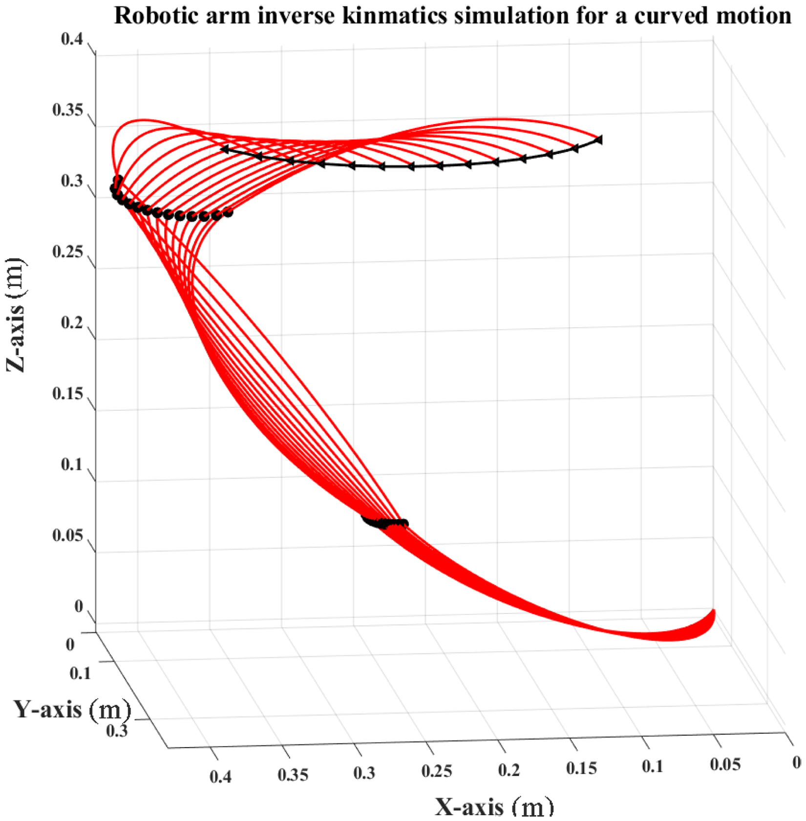
Manipulator inverse kinematics simulation for a curved motion.

Experiment of narrow pipeline crossing

To assess the efficacy of the path-following algorithm integrated with the backbone inverse kinematics as proposed in this study, an experimental setup featuring a narrow environment was devised. The performance of the proposed algorithm was validated through the manipulation of the robotic arm along with a predetermined path. A cable-driven soft manipulator system with over 15 degrees of freedom was developed to validate the proposed methodology. This manipulator encompasses four active degrees of freedom driven by motors and more than nine degrees of freedom resulting from its inherent structural flexibility.

The experimental setup, depicted in Figure 10, comprises a PC, a narrow environment simulation framework (NESF), a slide guide, and the manipulator system. The NESF is affixed to the slide guide. As the slide guide initiates movement, relative motion between the NESF and the manipulator system is enabled.

Figure 10.

The experiment system.

The soft manipulator's design can be divided into two main components. The first is flexible and primarily composed of silicon rubber that can be 3D printed. The second component is driven by motors, which control the length of each driving wire precisely through a screw guide mechanism. The 3D-printed main body is driven by power transmission elements. Considering the advantages outlined in the introduction, our design opted for a cable-driven mechanism. To enhance flexibility, the 3D-printed body features serrated structures on all four sides. Each of these structures has a through-hole for cable connection. Our design allows the cables to pass through these through-holes, thereby constraining them and enabling their shape to closely approximate that of the 3D-printed body. These four cables exhibit central symmetry, providing two degrees of freedom. Additionally, these cables are made of Dyneema, each capable of withstanding a weight exceeding 400 N. Moreover, Dyneema cables are not as sharp as metallic ones, reducing the risk of cutting into the 3D-printed body. Figure 11 represents the three-dimensional model of the soft manipulator.

Figure 11.

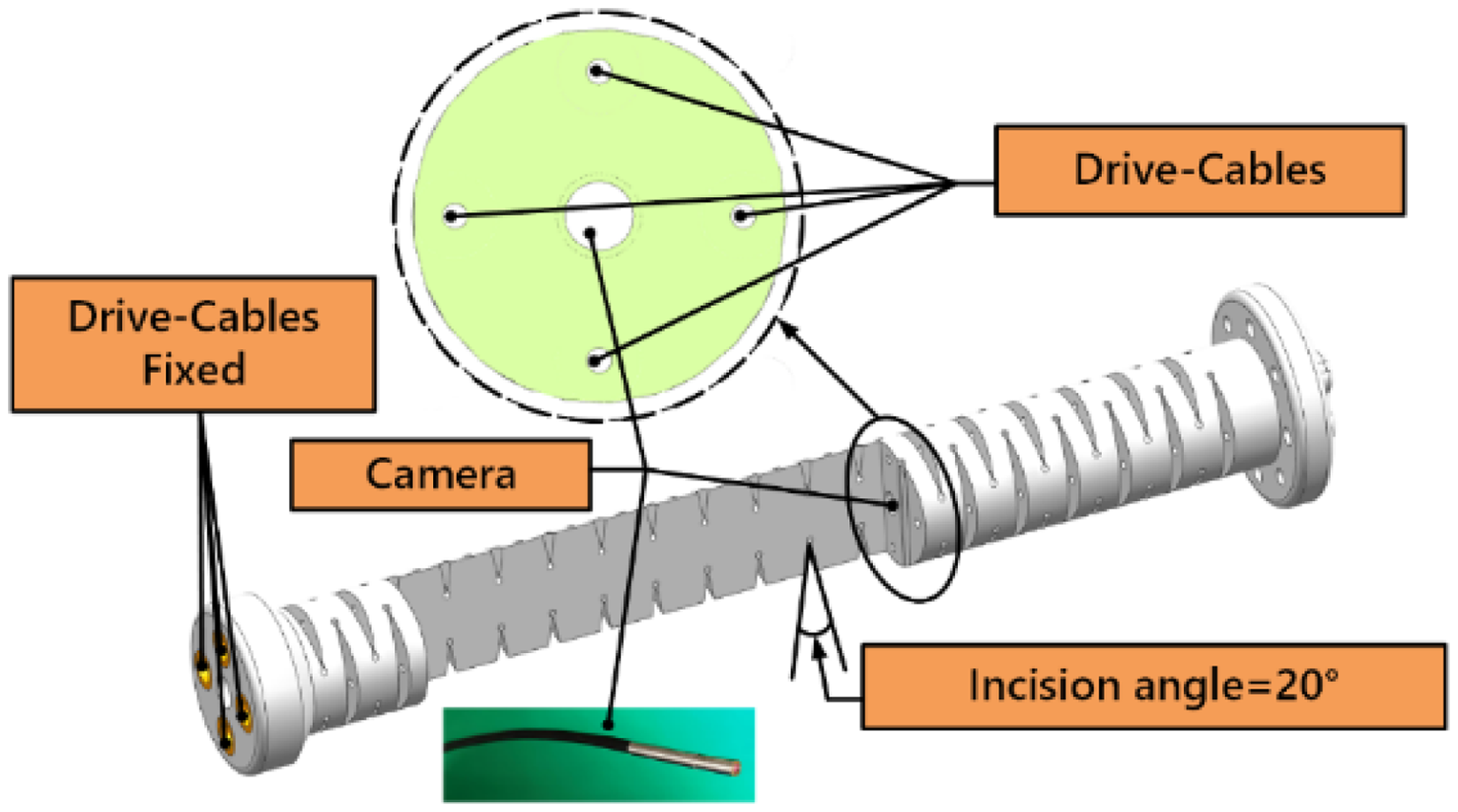
The three-dimensional model of the soft manipulator.

Figure 12 shows the experimental process. The manipulator enters the NESF through a 30-mm diameter round hole, and the camera at the end of manipulator can acquire the internal image information of NESF. Figure 13 reveals the final pose of manipulator. It is crucial for rescue and inspection tasks in narrow environments such as the aircraft fuel tank inspection or maintenance station space.

Figure 12.

Process of experiment.

Figure 13.

Final pose of manipulator.

The experiment results show that the proposed algorithm can meet the control requirements of the soft manipulator. It also reflects the extremely narrow space-crossing capability of the soft manipulator.

Conclusion

This paper introduces a novel algorithm to solve the inverse kinematics of a tendon-driven soft manipulator and a head traction path-following method based on the improved backbone inverse kinematics. Through simulation and experimentation, it was demonstrated that point-to-point inverse kinematics can be calculated within the manipulator's workspace using the improved backbone method, and the motion and driving parameters of the manipulator can also be determined. The head traction path-following algorithm enables complex path-following for soft or hyper-redundant manipulators. The arm presented in this paper, combined with the head traction algorithm, offers enhanced flexibility in applications such as space-based capture tasks. In future work, the head traction path-following algorithm, due to its lower computational complexity, will be considered in combination with real-time path-planning algorithms to achieve online target trajectory tracking.