Sage Journals: Discover world-class research

Abstract

The model predictive control trajectory planner is a popular and effective robot local motion planner. However, it is challenging to satisfy real-time requirements and implement them on embedded platforms due to their high complexity of solving and reliance on optimization solvers. This letter reports a lightweight and efficient two-stage solving algorithm for the model predictive control planner. Firstly, the general form of the model predictive control local planning problem was specified and simplified by the motion primitives. Then, a two-stage solving method of multi-layer perceptron pre-solving and particle swarm optimization re-optimizing is developed after splitting the cost function into two pieces. An multi-layer perceptron neural network was designed and trained offline to learn the solution of the model predictive control local planner without considering obstacles after selecting the inputs and outputs. Next, to accomplish obstacle avoidance, the particle swarm optimization algorithm re-optimizes the trajectory based on the outputs of the neural network. The experiment results demonstrate that the multi-layer perceptron-particle swarm optimization algorithm can quickly and accurately solve local planning problems, guiding robots to complete global paths with the same efficiency as expert solvers. The average solving time has been reduced by over 90%, enabling the robot to increase its control frequency or adopt higher-quality complex motion primitives. The multi-layer perceptron-particle swarm optimization algorithm can also be used for various robots and motion primitives, with a wide range of potential applications.

Keywords

Optimization algorithm model predictive control local planner motion planning multi-layer perceptron particle swarm optimization

Introduction

Motion planning is an important part of the robot system, bridging the gap between task execution and attitude control, which can be divided into global and local motion planning.¹ Local motion planning is responsible for guiding the robot to follow the global path efficiently and stably in shifting environments with a detailed kino-dynamics model.

Optimal-based methods, one type of commonly used method, transform the problem into a high-dimensional constrained optimization problem, such as the time elastic band (TEB),² model predictive control (MPC),¹ polynomial curve method,³ Bézier curve method,⁴ etc. In recent years, MPC local planner has been studied intensively and applied successfully on robots such as unicycles,⁵ unmanned aerial,^6,7 ground,^8,9 and ships¹⁰ vehicles. The forward prediction module enhances the completeness of trajectories and the stability of robots’ attitudes, while rolling optimization permits the planner to adapt to environmental changes and correct numerous errors, resulting in high-quality trajectories and an improvement in the robot’s stability and robustness. However, the MPC trajectory problem of robots is frequently a nonlinear optimization problem with multiple constraints, making it challenging to satisfy the real-time operation requirements. Incorporating the high-dimensional dynamic model and extending the predicted horizon can further enhance the planners’ performance, improving fast-moving⁸ and obstacle avoidance¹¹ abilities, even achieving aggressive driving in hard field environments,⁹ but increasing the solving complexity. Linearization is a commonly used technique to reduce optimization complexity but at the expense of solution quality.^8,11 The model predictive path integral (MPPI) method gets the optimal trajectory by parallel sampling calculation but puts requirements on hardware such as graph processing unit (GPU).⁹ Obstacle avoidance makes optimization more challenging to meet the real-time requirement. Hard constraint methods, such as the corridor method,⁷ add more constraints, while soft constraint methods complicate the optimization gradient.³ Nonlinear optimization problems usually require professional solving libraries such as IPOPT,¹² CasADi,¹³ and Acados,¹⁴ which are difficult to deploy on embedded platforms or lightweight operating systems. At the same time, the volume of high-performance computers is not conducive to the miniaturization of robots.

Sampling-based motion is another type of local planner that has good real-time performance at the expense of optimality. Some relevant technologies have been introduced to expedite the solving of the MPC local planner. First, motion primitive¹ uses a few parameters to encode long trajectories, to construct an efficient search tree to find the optimal trajectory.^15–17 The designated motion primitives generate the mapping between state and action space. Robot models were taken into account to assure trajectory implementability when designing motion primitives. Some researchers have used optimization techniques to find the optimal trajectory in the motion primitive space.¹⁸ Low space dimension enables quick optimization solutions, but multiple times solving the boundary value problem (BVP)^19,15,16 which converts motion primitives into trajectories, incurs additional time consumption. The second technique is the pre-solving dataset and look-up method.^20,21 Sample and solve to construct a trajectory dataset offline at first. In actual operation, the best trajectory can be quickly sought in the table. However, this method has two disadvantages: the solution quality is limited by the sampling precision. Reducing the sampling interval may increase the consumption of storage space and the difficulty of searching.²² Neural networks and imitation learning technologies have the potential to solve these issues. Using trajectory datasets as a guide, neural networks are capable of learning trajectory planning abilities due to their ability to match any nonlinear function. Currently, researchers have used neural networks to generate trajectories of robots with starting and ending points²³ or get the planning skills from human manipulation datasets.²⁴

The environment in which robots are located is continually changing, posing challenges to the input of environmental data into neural networks to accomplish obstacle avoidance. Some scholars use deep neural networks to process images²⁵ and point cloud²⁶ information to avoid obstacles, but they often need human teaching²⁴ or reinforcement learning.²⁶ Worse, the sampling and training are difficult and have no advantage in solving time. To accomplish obstacle avoidance, we adopted a re-optimization to construct a two-stage solution, which can simplify complex problems by focusing on different aspects during different stages of the solution,²⁷ producing effective solving.

The innovations of this letter can be summed up as follows: ① For the model prediction trajectory planner, a lightweight fast-solving algorithm called multi-layer perceptron and particle swarm optimization (MLP-PSO) is proposed with two stages: pre-solving and re-optimization, which does not require the complex code library and can be implemented on lightweight processors. ② An multi-layer perceptron (MLP) network was designed and trained to imitate the solvers without considering obstacles to achieve fast and accurate optimization. ③ Experiments have demonstrated that this algorithm can precisely solve MPC motion planning problems while reducing average optimization time by at least 90%, enabling the robot to increase its control frequency or adopt higher-quality complex motion primitives. Moreover, this algorithm is suitable for various robots and motion primitives.

The rest of the article is organized as follows. The “MPC local planner with motion primitive” section introduces the system framework and the construction of the MPC local planner with motion primitive. A detailed description of the MLP-PSO algorithm is presented in the ‘‘MLP-PSO algorithm” section. In the “Implementation and experimental robots” section, the implementation of the algorithm and experimental robots are represented. The experiments and results can be found in the “Results” section. The “Conclusion” section is the conclusion and future work of this article.

MPC local planner with motion primitive

This section begins with an overview of the mobile robot’s planning and control system. Then, establish and simplify the MPC local planning problem with motion primitives.

System framework

As depicted in Figure 1(a), the planning and control system of mobile robots often utilizes a hierarchical control structure. The global planner is responsible for finding feasible paths between the current location and the terminal. Based on the global path and the local cost map, the MPC local planner generates smooth trajectories and motion commands, avoiding time-varying obstacles. The motion controller executes commands and eliminates interference.

Figure 1.

(a) The whole framework of robot planning and control system (b) The framework of MPC local planner with MLP-PSO algorithm. MPC: model predictive control; MLP-PSO: multi-layer perceptron and particle swarm optimization.

Figure 1(b) shows the structure of the MPC local planner. After obtaining global path $p_{r e f}$ , local cost map, and robot state information from sensors and observers, the planner provides the optimal trajectory and control sequence through forward prediction and rolling optimization.

Motion primitive

The robot can be described by the following model:

\begin{aligned} \dot{x} = f (x, u) {h (x, u) = 0, \hat{h} (x, u) \leq 0, x \notin O} \end{aligned}

(1)

where

x \in X

represents the robot’s state and

u \in U

denotes its input. The

h

and

\hat{h}

represent the collection of state and input constraints, respectively. The last equation is the collision-free constraint, where

O

is the obstacle set.

If the robots’ inputs are generated according to specific rules of the motion primitive, the entire input sequence can be reproduced by solving the BVP problem with initial and terminal states. Then, the robot’s state sequence can be predicted by the kino-dynamic model. Therefore, there is a one-to-one correspondence between the trajectory and terminal system states.^1,6 Using terminal state as a motion primitive $ξ$ , we can build the mapping between $ξ$ and trajectories

S : ⟨ x_{0}, ξ ⟩ \to ⟨ \hat{u} (t), \hat{x} (t), {\hat{t}}_{f} ⟩

(2)

Model predictive local planning

The model predictive local planning problem can be expressed in the following general form of the MPC problem:

min_{x (t), u (t), t_{f}} J = Φ (x (t_{f})) + \int_{t_{0}}^{t_{f}} L (x (t), u (t), t_{f}) d t

(3)

By introducing the motion primitive, the complexity of the MPC problem can be reduced significantly by decreasing the number of optimization variables

min_{ξ} J = \bar{Φ} (ξ) + \int_{t_{0}}^{t_{f}} \bar{L} (ξ) d t

(4)

The cost function is determined by the purposes of the MPC problem. In general, the local planner ensures the robot can track global paths with reference speed, minimum energy, stable attitude, and collision-free. In practical use, the MPC problem needs to be expressed in a discrete form. The model predictive local planning problem is defined as follows:

\begin{aligned} min_{ξ (\cdot)} J (\cdot) = & \sum_{i = 1}^{N} {\bar{X}}_{i}^{'}^{T} H_{1} {\bar{X}}_{i}^{'} + {Δ ξ^{'}}^{T} H_{2} Δ ξ^{'} + H_{3} \sum_{i = 1}^{N} M A P_{X (i | k)} \end{aligned}

(5)

\begin{aligned} s.t. & X = (x, y, φ, v, \dot{v}, \ddot{v}, \dots, ω, \dot{ω}, \ddot{ω}, \dots)^{T}; X (0 | k) = {\hat{X}}_{k} \\ X^{'} = (x, y, φ)^{T}; {\bar{X}}_{i}^{'} = X^{'} (i | k) - {X^{'}}_{r e f} (i | k) \\ ξ = (v_{t e r}, ω_{t e r})^{T} \\ Δ ξ^{'} = (v_{t e r} (k), ω_{t e r} (k)) - (v_{m a x} (k), ω_{t e r} (k - 1)) \\ X (i | k) \in [X_{m i n}, X_{m a x}]; ξ \in [ξ_{m i n}, ξ_{m a x}] \\ G (X (i | k), ξ) = 0; F (X (i | k), ξ) < 0 \end{aligned}

Where

N

is the predicted horizon,

H_{1}, H_{2}, and H_{3}

is the cost coefficient matrix, and

M A P_{X (i | k)}

is the grid value of

(x, y)

on the local cost map. To assure the smoothness of the trajectory, the robot’s state vector should include velocity

v

, angular velocity

ω

, and their higher derivatives

(\dot{v}, \ddot{v}, \dots, \dot{ω}, \ddot{ω}, \dots)

in addition to the position vector

(x, y, φ)

. To concisely express the trajectory, the terminal velocity

v_{t e r}

and angular velocity

ω_{t e r}

are chosen as the motion primitives, while their higher-order derivatives default to 0 and can be disregarded.

Focus on the cost function, the first item enables the robot to follow the global path, while the second item enables the robot to drive at the reference speed with minimal turning consumption. Finally, the local cost map created and renewed by signed distance field (SDF) technology is introduced to implement gentle constraints for obstacle avoidance. The local cost map rasterizes the environment, resulting in the lower the grid value, the further it is to the obstacle. So minimizing this item can guide the robot away from obstacles. The difference between grids generates gradients for optimization.

MLP-PSO algorithm

In this section, the overview of the MLP-PSO algorithm is described first, followed by the details of each module.

Algorithm overview

The cost function of MPC local planner can be divided into two parts as follows:

J_{1} (\cdot) = \sum_{i = 1}^{N} {\bar{X}}_{i}^{'}^{T} H_{1} {\bar{X}}_{i}^{'} + {Δ ξ^{'}}^{T} H_{2} Δ ξ^{'}

(6)

J_{2} (\cdot) = H_{3} \sum_{i = 1}^{N} M A P_{X (i | k)}

(7)

J_{1} (\cdot)

ensures the robot can track the global path with a stable attitude, which is only related to robot states. While

J_{2} (\cdot)

lets the robot avoid obstacles, changing by the environment.

M A P_{X (i | k)}

is the cost value of

X (i | k)

in the local cost map. Figure 2 shows that the value of the whole cost function is the superposition of two parts.

Figure 2.

The cost function value of one real problem. The whole cost (under) is the superposition of states cost $J_{1} (\cdot)$ (upper left) and obstacles cost $J_{2} (\cdot)$ (upper right). The x and y axes represent $v_{t e r}$ and $ω_{t e r}$ in $ξ$ , respectively.

If the MPC problem is solved in an obstacle-free environment, the cost function degenerates into $J_{1} (\cdot)$ . And if the optimal trajectory exists in the obstacle-free area, $J_{2} (\cdot)$ can also be ignored. The MLP-PSO algorithm, as depicted in Figure 1(B) and Algorithm 1, is a two-stage approach for solving the MPC planning problem. An MLP neural network is introduced for the pre-solving stage, while the re-optimization stage is finished by the PSO algorithm.

MLP pre-solving stage: Mathematically, the optimal result of the MPC motion planner is a high-dimensional nonlinear function involving the system states, objective states, last motion primitive, and environment information. Since neural networks are capable of fitting any nonlinear function, they can be utilized to fit the result function. Inspired by imitation learning, an MLP neural network was trained to fit the control policy by treating the traditional planner as a ”teacher.” Ignoring the environment and concentrating on the $J_{1} (\cdot)$ , which is in a fixed state space, reduces the input dimension, training difficulty, and sampling complexity of the MLP network. We offline-trained an MLP network to learn the optimization result function of the $J_{1} (\cdot)$ under constraints, achieving fast, accurate, and space-efficient solving. The MLP neural network can provide motion primitives directly by taking the current state and target state of the robot as inputs.

PSO re-optimization: As Figure 2, the cost of obstacles provides new gradients for optimization, which can be optimized by the PSO. The particles are arbitrarily initialized near the MLP outcomes and converge to the global optimal solution of the whole function, relying on obstacle gradients. PSO is a discrete optimization technique that does not require cost functions to have continuous derivatives. Therefore, it has been used to optimize motion planning problems directly on the cost map,^6,28 avoiding the computational burden of converting the map into a continuous form.

The MLP-PSO algorithm solves local planning problems as shown in Algorithm 1. Firstly, we execute a forward traversal along the global path for a certain look-ahead distance from the present position of the robot to get the goal point (line 1). This look-ahead distance is determined by the robot’s maximum velocity and predictive horizon. Then, acquire the pre-solution by the MLP network (line 2). The MLP result is used for forward simulation to acquire predicted trajectories (line 3). If the trajectories are obstacle-free on the local cost map, the MLP result can be output directly to the control module (lines 4 and 5), and the optimization is finished. If not, the PSO algorithm is used for re-optimization to avoid obstacles (lines 7–23).

After obtaining the optimal motion primitive, the optimal control sequence is obtained by solving the BVP problem. Subsequently, the predicted trajectory is generated by applying this control sequence to the robot’s dynamic model, facilitating tasks such as collision detection and output visualization. If the predicted trajectory indicates a potential collision, the control sequence will not be sent to the motion controller, and an emergency stop command will be issued instead.

The MLP network and PSO algorithm can be decomposed into algebraic operations without the need for complex code libraries. Therefore, the MLP-PSO algorithm can be deployed on multiple platforms, including some lightweight processors.

Problem simplification

In this subsection, the MPC local planning problem is transformed into a simpler form.

First, according to the $S E (2)$ transformation of current position $(^{w} x_{c u r},^{w} y_{c u r})$ and attitude $^{w} R$ in world frame $W$ , the reference global path $(^{w} x_{r e f},^{w} y_{r e f})$ can be changed to local frame $L$ . The position of the robot in the local frame $^{l} X^{'} (k)$ is $(0, 0, 0)^{T}$ , which can be ignored in sampling.

\begin{matrix} [\begin{matrix} ^{l} x_{r e f} \\ ^{l} y_{r e f} \\ ^{l} φ_{r e f} \end{matrix}] = [\begin{matrix} \cos^{w} φ_{c u r} & \sin^{w} φ_{c u r} & 0 \\ - \sin^{w} φ_{c u r} & \cos^{w} φ_{c u r} & 0 \\ 0 & 0 & 1 \end{matrix}] [\begin{matrix} ^{w} x_{r e f} -^{w} x_{c u r} \\ ^{w} y_{r e f} -^{w} y_{c u r} \\ ^{w} φ_{r e f} -^{w} φ_{c u r} \end{matrix}] \end{matrix}

(8)

Second, the most critical task of the local planner is generating a trajectory along the global path. The look-ahead method is prevalent and efficient. According to Paden et al.,²⁹ Svec et al.,³⁰ and Mora and Tornero,³¹ robots can complete the path by tracking a point on the global path at a certain distance in front of them. This method significantly decreases the input dimension of the planner, enables the use of neural networks to plan, and simplifies sampling and training. Moreover, this method reduces constraints on trajectories and increases the optimization’s degree of freedom to generate better trajectories while decreasing the influence of poor-quality global paths.

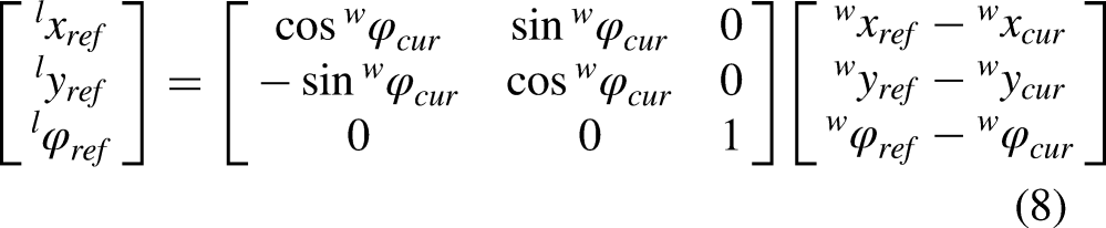
Thus, after two steps, the robot tracks a target point $^{l} {X^{'}}_{g o a l} = (^{l} x_{g o a l},^{l} y_{g o a l},^{l} φ_{g o a l})^{T}$ obtained from the global path to complete the global path in the local frame $L$ , as shown by the arrows in Figure 3(a). The $J_{1} (\cdot)$ cost function can be simplified as follows:

J_{1} (\cdot) =^{l} {\bar{X}}_{g o a l}^{' T} H_{1}^{l} {\bar{X}}_{g o a l}^{'} + {Δ ξ^{'}}^{T} H_{2} Δ ξ^{'}

(9)

\begin{aligned} ^{l} {\bar{X}}_{g o a l}^{'} =^{l} {X^{'}}_{g o a l} (k) -^{l} X^{'} (N | k) X^{'} = (x, y, φ)^{T} \end{aligned}

Figure 3.

Related figures about MLP-PSO algorithm: (a) The reachable position of the robot on a certain predicted horizon. Each arrow represents a goal $^{l} {\bar{X}}^{'}_{g o a l}$ . (b) The inputs, outputs, and structure of the MLP neural network. (c) The re-optimization process of the PSO algorithm for obstacle avoidance. The number represents the optimal trajectory found in the sequence. The shaded region denotes the extension of the obstacle. MLP: multi-layer perceptron; MLP-PSO: multi-layer perceptron and particle swarm optimization; PSO: particle swarm optimization.

MLP neural network

The global optimal solution for optimization problems is a function of the inputs and parameters. The existence of variable constraints, nonlinear links, and generation rules of motion primitives makes the analytical function of optimization problems either nonexistent or challenging to find and express. Thanks to imitation learning, the neural networks can directly adapt the result function and learn control policy from the result dataset, cloning the solution procedure. An MLP network was designed in this study.

Figure 3(b) depicts the structure of the MLP neural network, which has nine inputs and two outputs. The inputs are goal position $(^{l} x_{g o a l},^{l} y_{g o a l},^{l} φ_{g o a l})$ (Goal Pos, $3 \times 1$ ), reference velocity by setting ( $v_{r e f}$ , $1 \times 1$ ), last terminal angular velocity (Last $ω_{t e r}$ , $1 \times 1$ ), start velocity and acceleration (Start $(v, \dot{v})$ , $2 \times 1$ ), start angular velocity and angular acceleration (Start $(ω, \dot{ω})$ , $2 \times 1$ ). Start $(v, \dot{v})$ and $(ω, \dot{ω})$ are current states of robot. The outputs are the motion primitive composed of terminal velocity ( $v_{t e r}$ , $1 \times 1$ ) and terminal angular velocity ( $ω_{t e r}$ , $1 \times 1$ ). After determining the inputs and outputs of the neural network, hidden layers are added to form a complete structure. Based on the common expansion-contraction rule, after multiple tests, the established MLP neural network has six layers with a structure of 9-48-16-8-4-2. The activation function of the hidden layer is $R e L U$ , while $S i g m o i d$ is used for the output layer.

Algorithm 1:

MLP-PSO algorithm.

Input: robot states $\hat{X} (k)$ , global path, local cost map
Parameter: kino-dynamic model, cost function parameters
Output: terminal target states $ξ (k)$ , local trajectory $X (i \| k)$
1:	Obtain the goal ${X^{'}}_{g o a l}$ from the global path.
2:	Put $\hat{X} (k)$ and ${X^{'}}_{g o a l}$ into MLP to get result $ξ_{p r e} (k)$ .
3:	Obtain $X (i \| k)$ by using $ξ_{p r e} (k)$ for forward prediction.
4:	if predicted trajectory $X (i \| k)$ is collision-free then
5:	$ξ (k) = ξ_{p r e} (k)$ , return $ξ (k)$ , $X (i \| k)$
6:	else
7:	$ξ^{} = ξ_{p r e} (k), c^{} = J (X (i \| k), {X^{'}}_{g o a l}, ξ^{*}, M A P)$
8:	$Ξ \leftarrow$ Particles initialization nearby $ξ_{p r e} (k)$ .
9:	$ξ_{n}^{} \leftarrow ξ_{n}, c_{n}^{} \leftarrow \infty, δ_{n} \leftarrow r a n d, \forall n \in [1, s i z e (Ξ)]$
10:	for t = 1 to ITERS do
11:	for $ξ \in Ξ$ do
12:	Obtain trajectory $X (i \| k)$ by putting $ξ_{n}$ into robots' model for forward prediction.
13:	$c_{n} = J (X (i \| k), {X^{'}}_{g o a l}, ξ_{n}, M A P)$
14:	if $c_{n} < c_{n}^{*}$ then
15:	$c_{n}^{} = c_{n}, ξ_{n}^{} = ξ_{n}$
16:	end if
17:	if $c_{n} < c^{*}$ then
18:	$c^{} = c_{n}, ξ^{} = ξ_{n}$
19:	end if
20:	$δ_{n} = δ_{n} + k_{1} \cdot r a n d \cdot (ξ_{n}^{} - ξ_{n}) + k_{2} \cdot r a n d \cdot (ξ^{} - ξ_{n})$
21:	$ξ_{n} = ξ_{n} + δ_{n}$
22:	end for
23:	end for
24:	Obtain $X (i \| k)$ by using $ξ^{*}$ for forward prediction.
25:	$ξ (k) = ξ^{*}$ , return $ξ (k)$ , $X (i \| k)$
26:	end if

To satisfy the calculation of the MLP network, the inputs and outputs are normalized to $[0, 1]$ by the boundaries, which are determined by different methods. The boundary of the robot’s states (such as $v, ω$ ) can be obtained through theoretical analysis based on the capabilities of actuators such as motors. The pre-experiments find the coefficients of the cost function and the boundary of Goal Pos. As shown in Figure 3(a), for a certain predicted horizon, the reachable position of the robot should be a sector. The MAX look-ahead distance is determined by the MAX $v$ and $a$ of the robot, whereas the MAX angle the robot can rotate within a given time is limited by the MAX $ω$ .

Compared to traditional look-up methods, the MLP neural network’s result is continuous on state space, producing more accurate results by fitting for non-sampled points. And the MLP method only requires the storage of the network’s parameters (hundreds of floating-point numbers) without the need to store complex search trees or look-up tables, thereby saving a significant amount of space. The computation cost of forward propagation is also superior to that of searching in complex trees.

Sampling and training

The sampling space is a nine-dimensional space composed of neural network inputs. The sampling only needs to be carried out within the boundary, and points outside the sampling place can be normalized to the boundary. The sampling can be divided into two steps: first, uniform sampling to assure coverage, followed by adding white noise with a standard deviation as a sampling interval to points to improve randomness. Each sampling point can be converted into an MPC problem and solved by mature solvers such as IPOPT¹² to get the result.

The dataset can be divided into a training set and a testing set with a ratio of 7:3. The MLP neural network is trained with a weighted mean-square error (WMSE) loss on velocity and angular velocity based on backpropagation and batch training algorithms. The batch size was set to 200, and the training cycle was 1000. The lossfunction of training is

L o s s = w_{v} \cdot ‖ v_{d} - v_{n} ‖^{2} + w_{ω} \cdot ‖ ω_{d} - ω_{n} ‖^{2}

(10)

where

v_{d}

and

ω_{d}

are the command data in the training set, while

v_{n}

and

ω_{n}

are the outputs of the network. To maintain the stability of the robot’s orientation, we pay more attention to the

ω

error by setting the weighs

w_{v}

and

w_{ω}

as 1 and 2.

The MLP network employs the dataset as a teacher to imitate the solver. The trained MLP network can be regarded as a solver for a specific optimization problem.

PSO algorithm

PSO is an intelligent search technique that optimizes the cost function by utilizing the motion of particles. The discrete cost function can be optimized directly due to the direction of particles, which only depends on the values of the previous and subsequent iterations. The PSO algorithm suits the forward prediction-rolling optimization scheme of the MPC and has been widely used for solving nonlinear MPC problems.^28,32

The particle swarm is initialized randomly near the result of the MLP network, which is also the initial global optimal result (lines 7–9). Then, the optimal solution is searched through iteration. In each iteration, for each particle, the BVP problem is solved to get the full input sequence of the robot (line 12). Then, utilize the prediction model and cost function $J (\cdot)$ to get the cost (line 13). Through the comparison of costs, each particle’s and global optimal result are updated (lines 14–19). The optimization is stopped when the cost falls below the set value or hits the iteration limit. The optimal result is output to the control module for execution (line 25).

The process of a re-optimization is shown in Figure 3(c). It can be seen that as the optimization goes on, the robot’s trajectory moves away from obstacles, getting the optimal result considering obstacles. Because the MLP network produces approximations, the PSO algorithm can get the optimal result much more quickly than optimizing directly.

Implementation and experimental robots

In this section, we first outline the deployment steps of the MLP-PSO method onto the robot, followed by the presentation of the car-like robot and spherical robot used for testing.

Implementation

For any robot, the deployment of the MLPPSO method involves the following steps:

Establishing the robot model and selecting appropriate motion primitives based on the model.

Formulating the model predictive trajectory planning problem and simplifying it by motion primitives.

Determining system state boundaries and sampling rules to create multiple planning problems, solving them by mature solvers to obtain planning results and form the complete dataset.

Partitioning the dataset into training and testing sets for training the MLP neural network.

Deploying the trained MLP neural network and PSO algorithm on the robot platform.

By forming the new dataset, and adjusting the MLP network’s inputs and outputs, adaptation to more robots can be achieved, such as quadcopters in

S E (3)

space.

Car-like robot

The car-like robot is one of the most common unmanned ground vehicles (UGVs), which achieves free motion on the X-Y plane by changing the steering angle of the front wheels, as shown in Figure 4(a). To ensure the smoothness of the trajectory, Jerk limited trajectory (JLT)^33,34 is introduced as the motion primitive, and the terminal constraints of its BVP problem are the terminal velocity $v_{t e r}$ and angular speed $ω_{t e r}$ . Then, the kino-dynamic model of the robot can be expressed as follows:⁶

\begin{matrix} \dot{x} = v \cos φ, \dot{y} = v \sin φ, \dot{φ} = ω = v \cdot \sin δ / l \\ \dot{v} = α, \dot{α} = j, \dot{ω} = β, \dot{β} = j^{ω} \end{matrix}

(11)

\begin{aligned} v \in [v_{m i n}, v_{m a x}], α \in [α_{m i n}, α_{m a x}], j \in {0, j_{m i n}, j_{m a x}} \\ ω \in [ω_{m i n}, ω_{m a x}], β \in [β_{m i n}, β_{m a x}], j^{ω} \in {0, j_{m i n}^{ω}, j_{m a x}^{ω}} \end{aligned}

The state vector of the robot is

[x, y, φ, v, α, j, ω, β, j^{ω}]

. And the

v

α

, and

j

curves of a JLT trajectory are shown in Figure 4(b). The values of the jerk are

{m a x, m i n, 0}

. After integration, the

α

is continuous, and the

v

is continuous and smooth. When both

v

and

w

satisfy the constraints of JLT, the robot’s trajectories are very smooth. By introducing the requirement of minimum state transition time, acceleration and velocity trajectories can be efficiently computed using forward simulation,³⁴ avoiding the complexity of solving the BVP. After incorporating JLT into the MPC local planner, the PSO algorithm is utilized to solve optimization problems, similar to the application by Lai et al.⁶

Figure 4.

(a) The motion diagram of the car-like robot. (b) The $v$ , $α$ , and $j$ curves of a Jerk limited trajectory (JLT) trajectory.

Spherical robot

The spherical robot is an innovative type of special operation robot with large application potential in field exploration, security patrol, planet exploration, etc.³⁵ As shown in Figure 5(a), our laboratory has developed a spherical robot driven by a 2-DOF pendulum. By adjusting the output torque of two motors to adjust the position of the pendulum, the spherical robot can achieve motion on the X–Y plane.

Figure 5.

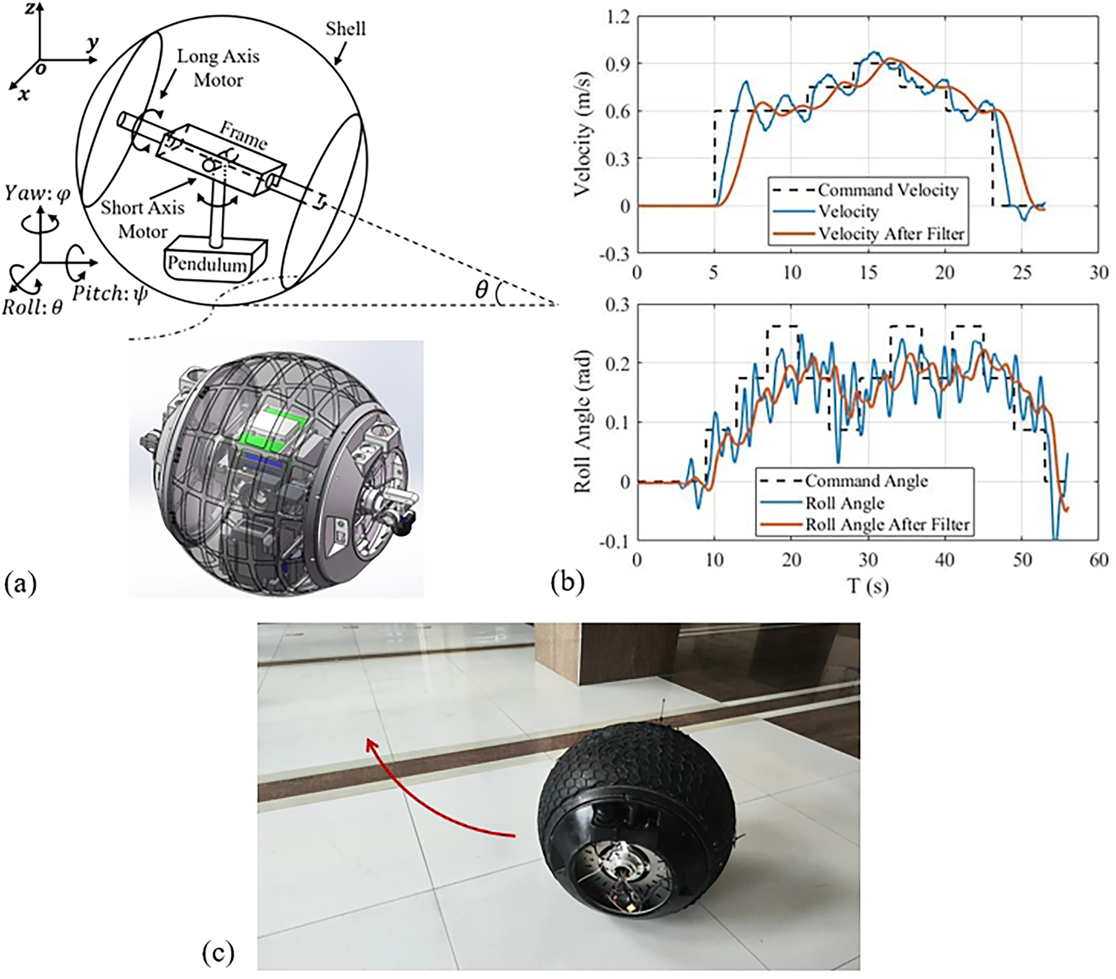
(a) The motion diagram and design drawing of the spherical robot. (b) The control effect of the attitude controller. (c) The physical drawing of the spherical robot and the real-world test scenario.

The characteristics of the spherical robot,^36,37 including strong nonlinearity, under-actuation, non-holonomic, and a high time latency, present challenges for the planning control system. It has been determined that the attitude controllers of velocity $v$ and roll angle $θ$ are necessary. As shown in Figure 5(b), even with the controllers, the attitude of the robot still has some fluctuations. Therefore, the robot’s dynamic model must be incorporated into the local motion planner. Due to the complexity of the controller and robot model, it is challenging to develop a theoretical model, which can’t be optimized in real time either. An ARX model is used to identify a simplified linear dynamic model of the cycle composed of the controller and robot, which is the control object of the motion planner. The complete kino-dynamic model is as follows:

\dot{x} = v \cos φ, \dot{y} = v \sin φ, \dot{φ} = ω = v \cdot \tan θ / r

(12)

\begin{aligned} \dot{x} = A \cdot x + B \cdot u, x = [v, \dot{v}, θ, \dot{θ}]^{T}, u = [v_{c m d}, θ_{c m d}]^{T} \\ x \in [x_{m i n}, x_{m a x}], u \in [u_{m i n}, u_{m a x}] \end{aligned}

where

A

and

B

are given by the system identification method.

θ

is the roll angle of the spherical robot. The whole state vector is

[x, y, φ, ω, v, \dot{v}, θ, \dot{θ}]

. The motion primitives are also the terminal velocity

v_{t e r}

and angle velocity

ω_{t e r}

. In which, the

ω_{t e r}

can be converted to

θ_{t e r}

through the formula

ω = v \cdot \tan θ / r

. The optimal control sequence is obtained by interpolating between the current states and motion primitive. The MPC local planning problem of the spherical robot is solved by IPOPT.¹² Obstacle avoidance is achieved by adding hard constraints to states.

Results

In this section, the details of the MLP training are presented first. Next, the solution accuracy of the MLP-PSO algorithm was evaluated using arbitrarily generated data. After deploying the algorithm to the car-like (in the simulator) and spherical robot (in the real world), the effect and time consumption of the MLP-PSO and traditional solvers (PSO for car and IPOPT for spherical) are compared experimentally. Two types of robots can verify the universality of the MLP-PSO algorithm, and the physical spherical robot experiment can verify the realistic feasibility. Subsequently, the spherical robot is used to evaluate the obstacle avoidance ability of the MLP-PSO algorithm.

Sampling, training, and testing all run in a single thread on a mini PC with an Intel i7-8559U CPU (2.70 GHz, quad-core 64-bit) and 32G RAM.

The MPC local planner runs at a frequency of 10 Hz on robots, which is a commonly used frequency of the local planner.^6,8,10 The frequency of the global planner is 1 Hz, so there might be multiple global paths in the resulting figure.

MLP training results

The predictive horizon of the MPC local planner is set to 2 s. After the offline sampling and generation of the dataset based on the pre-experiment parameters, two pre-solving MLP networks are trained for selected motion primitives of the car-like and spherical robot. Table 1 displays the dataset size, time consumption, and training error.

Table 1.

The details of MLP training.

Robot	Samples number			Time consumption $(s)$			Error on $v (m / s)$		Error on $ω (rad / s)$
Robot	Training set	Test set	All	Sampling	Training	All	RMSE	MAX	RMSE	MAX
Car-like robot	329275	141118	470393	14126.94	7537.43	21664.37	0.00401	0.01907	0.01448	0.09724
Spherical robot	167991	71996	239987	4718.75	3811.49	8530.24	0.00145	0.00570	0.01076	0.05676

MLP: multi-layer perceptron; RMSE: root mean square error.

After 1000 cycles of training, the root mean square error (RMSE) of velocity $v$ and angular velocity $ω$ on the test set are < 0.005 and 0.015. In comparison to the robot’s $v$ range $[0, 1]$ m/s and $ω$ range $[- 0.6, 0.6]$ rad/s, the error ratios are 0.5% and 1.25%, which are negligible. While the MAX error can reach 2% and 8% on $v$ and $ω$ . Because the MAX error occurs by accident, it is acceptable in applications. The total time consumption for sampling and training is about 6 and 2.5 hours, respectively, not high and meeting application requirements. As the car-like robot shows, when the model and motion primitives are more complex, more detailed sampling is required, and training time also increases.

Solution accuracy

In this section, 1000 random samples are generated in environments with and without obstacles to compare the MLP-PSO algorithm and traditional solvers (PSO or IPOPT, as mentioned above). The results are shown in Table 2. The results given by traditional solvers are regarded as ground truth.

Table 2.

The solution accuracy of multi-layer perceptron and particle swarm optimization (MLP-PSO) algorithm.

Robot	Scenario	Error on $v (m / s)$		Error on $ω (rad / s)$
Robot	Scenario	Average $^{a}$	MAX	Average	MAX
Car-like	Clear	0.00538	0.01875	0.01140	0.08426
Car-like	Obstacle	0.00457	0.00618	0.00330	0.03571
Spherical	Clear	0.00150	0.00452	0.00891	0.02648
Spherical	Obstacle	0.00013	0.00031	0.00502	0.01400

$*^{a}$ All average results were calculated from 1000 samples.

The obstacle-free scenario only requires the application of the MLP network, whereas the obstacle environment necessitates re-optimization with the PSO algorithm.

No matter what the robot is or whether there are obstacles in the environment, the average errors of velocity $v$ and angular velocity $ω$ are < 1% of the value range. The $v$ error is smaller, $0.5 %$ for the UGV and 0.1% for the spherical robot. The magnitude of the average error shows that the MLP-PSO solver achieves accuracy comparable to traditional solvers, meeting the required precision. Considering rare extreme situations, the MAX $v$ error is 2% of the value range, while for $ω$ is 7%, which is acceptable as MAX error occurs by chance. The interference of obstacles can be effectively resolved by PSO re-optimization, which can also decrease fitting errors of MLP, reducing the average errors. It can be seen that the complex motion primitives of car-like robots present greater challenges to the MLP-PSO, resulting in bigger errors. Such extreme errors occur sporadically and are acceptable in practical use, as even traditional solvers can exhibit the same level deviations.

Overall, accuracy tests demonstrate that the MLP-PSO algorithm satisfies the accuracy requirements necessary for practical implementation and can be implemented on robots for further testing.

Car-like robot experiment

The car-like robot completes multiple curved paths in a complex corridor environment by the simulator.

The reference velocity $v_{r e f}$ varies. The robot tries to complete the straight path at 1 m/s and achieve small radius non-skid turns at 0.8 m/s or even 0.6 m/s. Five experiments were conducted to eradicate randomness. The statistics that evaluate path completion, solving time, and the function running count are presented in Table 3 as the mean $\pm$ standard deviation. Figure 6(a) depicts the robot’s driving result, velocity, and angular velocity curve.

Figure 6.

(a) The diving result (blue line: global paths; red line: driving path), velocity curve, and angular velocity curve of the car-like robot with two different solvers. (b) The diving result (blue line: global paths; red line: driving path), velocity curve, and roll angle curve of the spherical robot with two different solvers.

Table 3.

The results of experiments.

Robot	Solver	Execution	Running	Average $ω$	Range of $ω$ or $θ$	Range of
Robot	Solver	time (s)	distance (m)	(rad/s)	(rad/s or $\circ$ )	solving time (ms)
Car-like	PSO	83.54 $\pm$ 2.54	94.25 $\pm$ 3.68	0.171 $\pm$ 0.011	[ $-$ 0.528, 0.571]	[8.394, 94.058]
Robot	MLP-PSO	81.64 $\pm$ 1.36	90.20 $\pm$ 1.32	0.166 $\pm$ 0.004	[ $-$ 0.518, 0.572]	[0.091, 7.763]
Spherical	IPOPT	56.91 $\pm$ 0.50	65.84 $\pm$ 1.10	0.185 $\pm$ 0.006	[ $-$ 17.86, 18.35]	[10.65, 82.91]
Robot	MLP-PSO	55.71 $\pm$ 0.23	64.63 $\pm$ 0.62	0.180 $\pm$ 0.002	[ $-$ 16.19, 20.29]	[0.063, 4.915]

Robot	Solver	Average solving time (ms)			Function runting count $^{a}$
Robot	Solver	All	MLP	MLP-PSO	All	MLP	MLP-PSO
Car-like	PSO	20.51 $\pm$ 6.961	–	–	4607	–	–
Robot	MLP-PSO	1.388 $\pm$ 1.370	0.142 $\pm$ 0.052	2.594 $\pm$ 0.920	4460	2193	2267
Spherical	IPOPT	15.89 $\pm$ 3.602	–	–	3104	–	–
Robot	MLP-PSO	0.272 $\pm$ 0.673	0.107 $\pm$ 0.037	2.827 $\pm$ 0.703	3047	2862	185

PSO: particle swarm optimization; MLP-PSO: multi-layer perceptron and particle swarm optimization; IPOPT: Interior Point OPTimizer, pronounced IP-Opt; MLP: multi-layer perceptron.

$*^{a}$ The function running counts come from all five time experiments that were conducted to eradicate randomness.

It can be seen from the results that the MLP-PSO algorithm can drive the robot along the global path with the same performance as the traditional solver, with no significant differences in statistics (errors < 5%) and curves. The curves demonstrate that the robot’s $v$ and $ω$ are continuous and smooth, satisfying the JLT constraints. As shown, the robot’s trajectory tends to move away from obstacles, proving that PSO re-optimization has achieved the designed function.

As for time consumption, the MLP-PSO algorithm is clearly superior. In total implementation time, the MLP-PSO algorithm is 93.2% less than traditional methods. The obstacle-free scenario only requires the MLP network, with an average solving time of 0.142 ms, which can be negligible. In obstacle scenarios, re-optimization is required, with an average total solving time of 2.594 ms, which is also 87.4% faster than traditional methods. Based on the function running count, it is evident that scenarios with and without obstacles are nearly equally represented. As a result, the final average solving time is approximately the mean of these two conditions. In extreme circumstances, the improvement is more obvious. Traditional methods may require around 95 ms maximum and can only plan at 10 Hz. While the MLP-PSO algorithm requires < 8 ms, enabling the local planner’s operating frequency to be increased to 20 Hz, 50 Hz, or even higher. This also allows for the use of more complex motion primitives to meet higher control demands.

From the trajectory, it can be observed that the complexity of the robot traversed areas varies, with both wide and narrow areas. The small solving time variance result indicates that complex environments with multiple obstacles do not significantly increase the solving time. The soft constraint obstacle avoidance method makes multiple obstacles generate more optimization gradients on the map rather than imposing complex constraints, which has minimal impact on the solving complexity.

The car-like robot experiment demonstrated the MLP-PSO solver’s significant advantage in reducing solving time compared to traditional solvers. This reduction greatly alleviates the load on the robot’s controller. Furthermore, the experimental results further confirmed that the MLP-PSO algorithm meets the accuracy requirements.

Spherical robot experiment

The spherical robot, shown in Figure 5(a), was utilized to conduct real physical experiments, which was designed and developed by our laboratory. The test scenario is also shown in Figure 5(c).

The task is an 8-figure multi-point patrol with eleven waypoints. The $v_{r e f}$ setting is the same as the car-like robot. Since the turns of the spherical robot are accomplished by adjusting roll angle $θ$ , some statistics and curves are changed to $θ$ . The results are illustrated in Table 3 and Figure 6(b).

The results indicate that the IPOPT solver and MLP-PSO algorithm can both solve the local planning problem, guiding the spherical robot to complete the patrol task effectively and in a stable state. There is no significant difference between the two methods’ statistics and result trajectories. Under the commands given by the MLP-PSO algorithm, the non-holonomic, non-linear, under-actuated, and critically stable spherical robot can achieve smooth acceleration and deceleration based on the actual conditions in order to increase efficiency. The roll angle can also be adjusted on command to achieve turning without violent oscillation or divergence.

The average solving time for the MLP-PSO algorithm is 0.107 and 2.827 ms in obstacle-free and obstacle environments, which is 99.3% and 82.2% less than traditional methods. The benefits are readily apparent. From the count of function runs, it can be seen that there are fewer obstacles in the spherical robot experiment. Thus, the overall average solving time decreases substantially (around 98.3%). Furthermore, the maximum solving time is < 5 ms (a decrease of 94.1%), which is a significant improvement over the IPOPT solver (64.03 ms).

In conclusion, experiments on car-like and spherical robots demonstrate that the MLP-PSO algorithm can effectively solve the model-predictive trajectory planning problem to guide the robot running along the global path with the same performance as the traditional solver, reducing the solving time by more than 82% even in complex environments. The substantial reduction in solving time highlights the superiority of the MLP-PSO algorithm compared to traditional methods. Tests conducted on two different types of robots demonstrate the algorithm’s general applicability, while the real-world experiment with the spherical robot validates its practical feasibility and superiority.

Obstacle avoidance experiment

In the experiments, two kinds of robots successfully avoided obstacles, especially the car-like robot running in the narrow corridor. From Figure 6(a), it is evident that the global path (blue line) did not account for the width of the robot, which may guide the robot to turn very near to the obstacle and cause collisions. The PSO algorithm re-optimized the trajectory to guide the robot away from the obstacle when it reached the turning point. After moving away from obstacles, the robot returned to the global path quickly. In conclusion, the MLP-PSO algorithm can achieve obstacle avoidance, and the soft constraint scheme is effective.

Conclusion

This article proposes a two-stage solving method called MLP-PSO for model predictive trajectory planners, addressing the challenges posed by complex models and long predicted horizons. At first, to quickly solve the standard MPC planning problem, an MLP neural network was trained on an offline dataset to imitate the solver without considering obstacles. Then, the obstacle avoidance task is accomplished by the PSO algorithm employed for re-optimization. Experiments have demonstrated that the solving quality of the MLP-PSO algorithm is identical to that of traditional solvers. Guided by the commands from the MLP-PSO algorithm, robots can effectively complete global paths while satisfying the predetermined requirements of the local planner. The MLP-PSO algorithm has a significant advantage in solving complexity and time consumption than the traditional method, reducing the average solving time by > 90%. The maximum solving time is < 10 ms, making it possible to improve moving performance by increasing the planning frequency to 20 Hz and higher or adopting higher-quality complex motion primitives.

Moreover, the MLP-PSO algorithm is suited for various robots and motion primitives. As for application, the MLP-PSO algorithm has a notable advantage in that it does not rely on code libraries, allowing MPC local planners to be deployed on low-performance processors and embedded platforms. This helps to achieve lightweight, miniaturization, and cost reduction of robots.

MLP-PSO offers a potential optimization method for complex MPC planning problems that cannot be solved in real time on robot platforms. We will try this application in the future. In addition, the application field of the MLP-PSO algorithm can be broadened by increasing the prediction horizon, adding robot and motion primitive types, and integrating dynamic models and constraints.

Footnotes

Declaration of conflicting interests

The author(s) declared no potential conflicts of interest with respect to the research, authorship, and/or publication of this article.

Funding

The author(s) disclosed receipt of the following financial support for the research, authorship, and/or publication of this article: This work is supported by the Rotunbot (Hangzhou) Technology Co., Ltd fund and the Zhejiang University Global Partnership Fund.

ORCID iDs

Xiaoqing Guan

Ziang Zhang

Yixu Wang

References

Howard

Pivtoraiko

Knepper

, et al. Model-predictive motion planning: Several key developments for autonomous mobile robots. IEEE Robot Autom Maga 2014; 21: 64–73.

Rsmann

Hoffmann

Bertram

. Kinodynamic trajectory optimization and control for car-like robots. In: 2017 IEEE/RSJ international conference on intelligent robots and systems (IROS).

Yang

Wang

, et al. Whole-body real-time motion planning for multicopters. In: 2021 IEEE international conference on robotics and automation (ICRA). IEEE, pp.9197–9203.

Yang

Sukkarieh

. An analytical continuous-curvature path-smoothing algorithm. IEEE Trans Robot 2010; 26: 561–568.

Ulrich

Borenstein

. VFH+: reliable obstacle avoidance for fast mobile robots. In: Proceedings. 1998 IEEE international conference on robotics and automation (Cat. No.98CH36146), pp.1572–1577 vol.2. DOI:10.1109/ROBOT.1998.677362.

Lai

Lan

Chen

. Model predictive local motion planning with boundary state constrained primitives. IEEE Robot Autom Lett 2019; 4: 3577–3584.

Zhou

, et al. Cmpcc: corridor-based model predictive contouring control for aggressive drone flight. In: International symposium on experimental robotics (ISER 2020). ISBN 978-3-030-71150-4, pp.37–46. DOI:10.1007/978-3-030-71151-1_4.

Fnadi

Plumet

Benamar

. Model predictive control based dynamic path tracking of a four-wheel steering mobile robot. In: 2019 IEEE/RSJ international conference on intelligent robots and systems (IROS). pp.4518–4523. DOI:10.1109/IROS40897.2019.8967627.

Williams

Drews

Goldfain

, et al. Aggressive driving with model predictive path integral control. In: 2016 IEEE international conference on robotics and automation (ICRA). pp.1433–1440. DOI:10.1109/ICRA.2016.7487277.

10.

Zhu

Gan

, et al. A hybrid control strategy of 7000 m-human occupied vehicle tracking control. IEEE Trans Intell Vehicles 2020; 5: 251–264.

11.

Lindqvist

Mansouri

Agha-mohammadi

, et al. Nonlinear MPC for collision avoidance and control of UAVs with dynamic obstacles. IEEE Robot Autom Lett 2020; 5: 6001–6008.

12.

Wächter

Biegler

. On the implementation of an interior-point filter line-search algorithm for large-scale nonlinear programming. Math Program 2006; 106: 25–57.

13.

Andersson

JAE

Gillis

Horn

, et al. CasADi – a software framework for nonlinear optimization and optimal control. Math Program Comput 2019; 11: 1–36.

14.

Verschueren

Frison

Kouzoupis

, et al. acados – a modular open-source framework for fast embedded optimal control. Math Program Comput 2021. DOI: https://doi.org/10.1007/s12532-021-00208-8.

15.

Paranjape

Meier

Shi

, et al. Motion primitives and 3D path planning for fast flight through a forest. Int J Rob Res 2015; 34: 357–377.

16.

Lopez

How

. Aggressive 3-D collision avoidance for high-speed navigation. In: ICRA. pp.5759–5765.

17.

Schwesinger

Rufli

Furgale

, et al. A sampling-based partial motion planning framework for system-compliant navigation along a reference path. In: 2013 IEEE intelligent vehicles symposium (IV). IEEE, pp.391–396.

18.

Ferguson

Howard

Likhachev

. Motion planning in urban environments: Part I. In: 2008 IEEE/RSJ international conference on intelligent robots and systems. pp.1063–1069. DOI:10.1109/IROS.2008.4651120.

19.

Mueller

Hehn

D’Andrea

. A computationally efficient motion primitive for quadrocopter trajectory generation. IEEE Trans Robot 2015; 31: 1294–1310.

20.

Liniger

Domahidi

Morari

. Optimization-based autonomous racing of 1: 43 scale RC cars. Optim Contr Appl Method 2015; 36: 628–647.

21.

Yang

Sreenath

Michael

. A framework for efficient teleoperation via online adaptation. In: 2017 IEEE international conference on robotics and automation (ICRA). IEEE, pp. 5948–5953.

22.

Frazzoli

Dahleh

Feron

. Maneuver-based motion planning for nonlinear systems with symmetries. IEEE Trans Robot 2005; 21: 1077–1091.

23.

Lin

Wang

Gao

, et al. Flying through a narrow gap using neural network: an end-to-end planning and control approach. In: 2019 IEEE/RSJ international conference on intelligent robots and systems (IROS). IEEE, pp.3526–3533.

24.

Akhloufi

. Learning to drive by imitation: an overview of deep behavior cloning methods. IEEE Trans Intell Vehicles 2020; 6: 195–209.

25.

Saleh

Attia

Hossny

, et al. Local motion planning for ground mobile robots via deep imitation learning. In: 2018 IEEE international conference on systems, man, and cybernetics (SMC). IEEE, pp.4077–4082.

26.

Zhang

Kahn

Levine

, et al. Learning deep control policies for autonomous aerial vehicles with MPC-guided policy search. In: 2016 IEEE international conference on robotics and automation (ICRA). IEEE, pp.528–535.

27.

Eiras

Hawasly

Albrecht

, et al. A two-stage optimization-based motion planner for safe urban driving. IEEE Trans Robot 2021; 38: 822–834.

28.

Zuo

Yang

Zhang

, et al. Lane-associated MPC path planning for autonomous vehicles. In: 2019 Chinese control conference (CCC). pp.6627–6632. DOI:10.23919/ChiCC.2019.8866609.

29.

Paden

Cap

Yong

, et al. A survey of motion planning and control techniques for self-driving urban vehicles. IEEE Trans Intell Vehicles 2016; 1: 33–55.

30.

Svec

Schwartz

Thakur

, et al. Trajectory planning with look-ahead for unmanned sea surface vehicles to handle environmental disturbances. In: 2011 IEEE/RSJ international conference on intelligent robots and systems. pp.1154–1159. DOI:10.1109/IROS.2011.6095021.

31.

Mora

Tornero

. Predictive and multirate sensor-based planning under uncertainty. IEEE Trans Intell Transp Syst 2015; 16: 1493–1504.

32.

Chu

Guo

, et al. Cooperative adaptive cruise control strategy optimization for electric vehicles based on SA-PSO with model predictive control. IEEE Access 2020; 8: 225745.

33.

Erkorkmaz

Altintas

. High speed CNC system design. Part I: jerk limited trajectory generation and quintic spline interpolation. Int J Mach Tool Manuf 2001.

34.

Macfarlane

Croft

. Jerk-bounded manipulator trajectory planning: design for real-time applications. IEEE Trans Rob Autom 2003; 19: 42–52.

35.

Liu

Sun

Jia

. A family of spherical mobile robot: driving ahead motion control by feedback linearization. In: 2008 2nd international symposium on systems and control in aerospace and astronautics. pp.1–6. DOI:10.1109/ISSCAA.2008.4776275.

36.

Vrunda

Joshi , et al. Design and analysis of a spherical mobile robot. Mech Mach Theory 2010; 45: 130–136.

37.

Wang

Guan

, et al. Fuzzy PID controller based on yaw angle prediction of a spherical robot. In: 2021 IEEE/RSJ international conference on intelligent robots and systems (IROS). pp.3242–3247. DOI:10.1109/IROS51168.2021.9636425.

Multi-layer perceptron-particle swarm optimization: A lightweight optimization algorithm for the model predictive control local planner

Abstract

Keywords

Introduction

MPC local planner with motion primitive

System framework

Motion primitive

Model predictive local planning

MLP-PSO algorithm

Algorithm overview

Problem simplification

MLP neural network

Sampling and training

PSO algorithm

Implementation and experimental robots

Implementation

Car-like robot

Spherical robot

Results

MLP training results

Solution accuracy

Car-like robot experiment

Spherical robot experiment

Obstacle avoidance experiment

Conclusion

Footnotes

Declaration of conflicting interests

Funding

ORCID iDs

References