AUV path planning based on improved IFDS and deep reinforcement learning

Abstract

Existing autonomous underwater vehicle (AUV) path planning algorithms are rapidly developing and perform well in solving optimal paths. However, the performance of these algorithms in real environments is significantly worse than that in simulated environments due to the influence of currents in real marine environments. To this end, this paper proposes an algorithm that improves the fusion of perturbed flow field and deep reinforcement learning and adds the influence of random currents to the environment, which further improves the overall accuracy of AUV obstacle avoidance in dynamic environments and enhances the AUV's adaptability to the real environment. This study also compares the results obtained using four fused deep reinforcement learning algorithms simulated in different scenarios, and the results show that the proposed algorithm can enable AUV to realize dynamic path planning in unknown environments.

Introduction

Autonomous underwater vehicles (AUVs) have been widely used in underwater rescue, unknown water exploration, and hydrological observation. ¹ With the continuous exploration of human beings into marine resources, AUVs have become the main tool for exploring the ocean. ² How to realize dynamic obstacle avoidance and calculate the optimal path of AUV in an unknown environment has become a hot research topic. ³ Currently, the main algorithms for path planning are Dijkstra's algorithm, A* algorithm, ⁴ ant colony algorithm, ⁵ genetic algorithm, particle swarm optimization algorithm, ⁶ artificial potential field method, ⁷ and reinforcement learning algorithm. ⁸

The origin of reinforcement learning algorithms can be traced back to 1911 when Thorndike proposed the Law of Effect: a behavior that makes an animal feel comfortable in a certain scenario enhances the association (reinforcement) with this scenario, and when this scenario is reproduced, this behavior of the animal is more likely to be reproduced; and the reverse is true. In 1956, Bellman ⁹ proposed the dynamic planning method. In 1977, Werbos ¹⁰ proposed adaptive dynamic planning methods. Until the late 1980s and early 1990s, artificial intelligence, machine learning, and other technologies began to be widely used, and reinforcement learning began to receive attention. In 1988, Sutton et al. ¹¹ proposed the temporal difference (TD) algorithm and in 1992 Watkins et al. ¹² proposed the Q-learning algorithm. Rummery et al. ¹³ proposed the SARAS algorithm in 1994, Bersakas et al. ¹⁴ proposed a neural dynamic programming method for solving optimal control in stochastic processes in 1995, Kocsis et al. ¹⁵ proposed the confidence upper tree algorithm in 2006, Lewis et al. ¹⁶ proposed the adaptive dynamic programming algorithm for feedback control in 2009, 2014 Silver et al. ¹⁷ proposed deterministic policy gradient (DPG) algorithm, 2016 Google DeepMind ¹⁸ proposed A3C method.

Deep learning is a type of neural network technology. Deep learning can perceive, but cannot make decisions; while reinforcement learning can make decisions, but cannot perceive. Deep learning is a type of artificial neural network that uses training samples as input to the network and solves problems through the network's own learning ability. Reinforcement learning is a kind of unsupervised algorithm, its main idea is to let the network through the environment of random action learn the strategy and finally get the optimal strategy, to solve the problem. The combination of the two has made great progress in theory, so deep learning and reinforcement learning are combined to generate a new type of learning algorithm, namely deep reinforcement learning, whose basic idea is to allow the network to randomly draw samples from the environment and train itself to solve a specific problem. It is a method for solving a series of decision-making problems by applying deep learning algorithms to reinforcement learning problems. Behnaz Hadi ¹⁹ proposed two new methods for end-to-end motion planning and control of AUVs using deep reinforcement learning algorithms with the help of actor-critic structure. Literature ²⁰ proposed a hierarchical deep Q-network (HDQN) approach for 3D path planning of AUVs and introduced the idea of an artificial potential field to improve the sparse reward problem.

For the avoidance of complex obstacles on the opposite side, literature ²¹ first proposed the interfered fluid dynamical system (IFDS) method, which is simple in modelling, small in computation, and easy to deal with complex terrain and different obstacles. In this paper, we combine the improved IFDS with a deep reinforcement learning algorithm and add the influence of ocean currents, hoping to improve the planning capability of AUV further. The structure of this paper is as follows: “Algorithm description” introduces the algorithms used in this study, “Experimental work and results” discusses the simulation results, and “Conclusion” concludes the paper.

The IIFDS-DRL algorithm proposed in this study combines an enhanced perturbation flow field model with deep reinforcement learning techniques to optimize AUV operations in random ocean currents. Its key contributions include:

Path Planning Optimization: The IIFDS-DRL algorithm efficiently plans paths in complex underwater environments and dynamically adjusts to changing flow conditions, thereby enhancing the efficiency and safety of mission operations.

Enhanced Autonomous Navigation: Leveraging deep reinforcement learning, the algorithm enables real-time learning and optimization of obstacle avoidance strategies, ensuring rapid responses to variable dynamic obstacles and maintaining operational safety and stability.

Improved Mission Efficiency: Compared to traditional methods such as A* algorithm, ant colony optimization, and rapidly-exploring random tree (RRT) algorithm, the IIFDS-DRL algorithm demonstrated superior efficiency and accuracy in path planning during experimental validations, effectively supporting various AUV mission operations in challenging underwater environments.

Practical Utility and Application Prospects: Beyond academic research, the algorithm offers innovative technical solutions for practical applications in fields such as marine science research and resource exploration, advancing the capabilities and applications of autonomous underwater robotics.

Algorithm description

Improved IFDS (IIFDS)

Algorithm flow

One way to depict obstacles is as standard convex bodies. ²² Buildings and hills are examples of topographical impediments that can be reduced to rectangles, cones, cylinders, hemispheres, or combinations of these shapes. Motion obstructions in the form of incursions can be visualized as balls. A barrier can be represented uniformly as:

$$\mathrm{\Gamma }(\xi )={\left({\displaystyle \frac{x-x_0}{a}}\right)}^{2d}+{\left({\displaystyle \frac{y-y_0}{b}}\right)}^{2e}+{\left({\displaystyle \frac{z-z_0}{c}}\right)}^{2f}$$

(1)

In the formula $\xi =(x,y,z)$ is the position of the intelligent body, and ${\xi }_0=(x_0,y_0,z_0)$ is the center of the obstacle, and $a,b,c$ is the length of the axis of the obstacle, and $d,e,f$ is the shape parameter. After modeling the environment, it is assumed that the target point is ${\xi }_d=(x_d,y_d,z_d)$ and the number of obstacles is K. $d=\sqrt{{(x-x_d)}^2+{(y-y_d)}^2+{(z-z_d)}^2}$ is the distance between the smart body and the target point.

Using a matrix $\overline{M}$ to represent the barrier's effect on the original fluid:

$$\overline{M}=\sum _{k=1}^K{\omega }_k{M}_k$$

(2)

Where ${\omega }_k$ is the weighting factor of the kth obstacle, and $M_k$ is the interference matrix of the kth obstacle.

$${\omega }_k=\{\begin{array}{cc}1& K=1\\ \prod _{i=1,i\ne k}^K{\displaystyle \frac{({\mathrm{\Gamma }}_i-1)}{({\mathrm{\Gamma }}_i-1)+({\mathrm{\Gamma }}_k-1)}}& K\ne 1\end{array}$$

(3)

$$M_k=I-{\displaystyle \frac{n_k{n}_k^T}{{|{\mathrm{\Gamma }}_k|}^{1/{\rho }_k}{|n_k|}^2}+{\displaystyle \frac{t_k{n}_k^T}{{|{\mathrm{\Gamma }}_k|}^{1/{\sigma }_k}|t_k||n_k|}}}$$

(4)

In the above equation ${\mathrm{\Gamma }}_k$ , the ${\mathrm{\Gamma }}_i$ is the barrier equation, and I is the attraction matrix, and $-n_k{n}_k^T/|{\mathrm{\Gamma }}_k{|}^{1/{\rho }_k}|n_k{|}^2$ is the repulsion matrix, and $t_k{n}_k^T/|{\mathrm{\Gamma }}_k{|}^{1/{\sigma }_k}|t_k||n_k|$ is the tangential matrix. ${\rho }_k$ is the repulsion coefficient, the ${\sigma }_k$ is the tangential coefficient, and $n_k=[\mathrm{\partial }{\mathrm{\Gamma }}_k/\mathrm{\partial }x,\mathrm{\partial }{\mathrm{\Gamma }}_k/\mathrm{\partial }y,\mathrm{\partial }{\mathrm{\Gamma }}_k/\mathrm{\partial }z{]}^T$ is the normal vector, and $t_k$ is the tangent vector. According to the following equation:

$$\{\begin{array}{c}{t}_{k,1}={\left[{\displaystyle \frac{\mathrm{\partial }{\mathrm{\Gamma }}_k}{\mathrm{\partial }y},-{\displaystyle \frac{\mathrm{\partial }{\mathrm{\Gamma }}_k}{\mathrm{\partial }x},0}}\right]}^T\\ t_{k,2}={\left[{\displaystyle \frac{\mathrm{\partial }{\mathrm{\Gamma }}_k}{\mathrm{\partial }x}{\displaystyle \frac{\mathrm{\partial }{\mathrm{\Gamma }}_k}{\mathrm{\partial }z},{\displaystyle \frac{\mathrm{\partial }{\mathrm{\Gamma }}_k}{\mathrm{\partial }y}{\displaystyle \frac{\mathrm{\partial }{\mathrm{\Gamma }}_k}{\mathrm{\partial }z},-{\left({\displaystyle \frac{\mathrm{\partial }{\mathrm{\Gamma }}_k}{\mathrm{\partial }x}}\right)}^2-{\left({\displaystyle \frac{\mathrm{\partial }{\mathrm{\Gamma }}_k}{\mathrm{\partial }y}}\right)}^2}}}}\right]}^T.\end{array}$$

(5)

Thus, any tangential vector can be expressed as:

$$t_k^{\mathrm{\prime }}=[\cos {\theta }_k,\sin {\theta }_k,0{]}^T$$

(6)

In the inertial system:

$$t_k={\mathrm{\Omega }}_T^I{t}_k^{\mathrm{\prime }}$$

(7)

Where ${\mathrm{\Omega }}_T^I$ is the coordinate transformation matrix from the tangent reference system to the inertial system.

Consider dynamic barriers to obtain the perturbed fluid velocity:

$$\overline{u}=\overline{M}(u-v)+v$$

(8)

$V$ is the total velocity of the obstacle, equation: ²³

$$V=\sum _{k=1}^K{\omega }_k\exp \left({\displaystyle \frac{-({\mathrm{\Gamma }}_k-1)}{{\lambda }_k}}\right)v_k$$

(9)

${\lambda }_k$ as a constant. Finally, the next planning point is obtained:

$$P_{t+1}=P_t+\overline{u}\cdot \mathrm{\Delta }T$$

(10)

$\mathrm{\Delta }T$ is the sampling time.

Improvement advantage

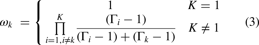
IFDS flows around an object often only in one plane, IIFDS adds a tangential matrix that can be varied by parameters to flow around the object in all directions. The improved rendering is shown in Figure 1.

Figure 1.

(a) IFDS and (b) IIFDS.

Deep reinforcement learning

The deep reinforcement learning algorithm used in this paper is combined with IIFDS to deep reinforcement learning algorithm to adapt to the environment in real time and automatically adjust the parameters of IIFDS. In this paper, four classical algorithms of deep reinforcement learning are used, which are DDPG, PPO, TD3, and SAC. The overall structure of the study is shown in Figure 2.

Figure 2.

Overall structure.

DDPG

The model consists of a four-layer neural network. ²⁴ Actor's current network is based on the agent's state $s_t$ to select the current behavior $a_t$ ，and the critic's current network is based on the current state $s_t$ , and the current action to compute the Q value. Similarly, the computational steps of the actor target network and critic target network are the same, the difference is that the network parameters are updated at different times, the parameters of the Actor target network and Critic target network are updated periodically, while the actor's current network and the critic's network are updated in real-time. The schematic diagram of the DDPG neural network combination update is shown in Figure 3.

Figure 3.

DDPG.

${\theta }^{\mu }$ is the actor's current network parameter, and the action selection formula is:

$$a_t=\mu (s_t|{\theta }^{\mu })$$

(11)

The Q-value of critic's current network is calculated using Bellman's equation:

$$Q^{\mu }(s_t,a_t)=E(r_t+\gamma Q^{\mu }(s_{t+1},\mu (s_{t+1})))$$

(12)

Once the values of the actor's current network and the critic's current network are known, the DDPG pair updates the parameters of the current network according to the target network. The current network is approximately better, the smaller the loss function. The loss function is calculated in the form of gradient descent with equation (13).

$$\mathrm{Loss}={\displaystyle \frac{1}{N}\sum _i(y_i-Q(s_i,a_i|{\sigma }^Q){)}^2}$$

(13)

Where $y_i$ is calculated from the objective function:

$$y_i=r_i+\gamma Q^{\mathrm{\prime }}(s_{i+1},{\mu }^{\mathrm{\prime }}(s_{i+1},|{\theta }^{{\mu }^{\mathrm{\prime }}})|{\theta }^{Q^{\mathrm{\prime }}})$$

(14)

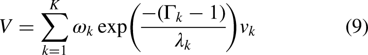
Use the U function to make a measure of the current network's strengths and weaknesses:

$$U_{\beta }(\mu )=\int {\rho }^{\beta }(s)Q^{\mu }(s,\mu (s))ds=E_{s\sim {\rho }^{\beta }}{Q}^{\mu }(s,\mu (s))$$

(15)

The gradient descent method is used to find the optimal parameters of the network with the expression as in equation (16):

$${}_{{\sigma }^{\mu }}{U}_{\beta }(\mu )E_{s\sim {\rho }^{\rho }}[{\begin{array}{c}Q(s,d|{\theta }^Q){|}_{a=\mu (s)}\end{array}}_{{\sigma }^{\mu }}\mu (s|{\theta }^{\mu })]$$

(16)

The updating formula for the target network parameters is shown in equations (17) and (18):

$${\theta }^{\mu }=\tau {\theta }^{\mu }+(1-\tau ){\theta }^{\mu }$$

(17)

$${\theta }^Q=\tau {\theta }^{\mu }+(1-\tau ){\theta }^Q$$

(18)

PPO

PPO is characterized by self-adaptation and good stability. ²⁵ It is a policy gradient algorithm. In practice, it is difficult to form an effective strategy because the difference between old and new strategies is too large. The method can iteratively update a small number of samples during multiple rounds of training, thus effectively solving the problems of difficulty in determining the step size and large update bias. The framework of the PPO algorithm is shown in Figure 4.

Figure 4.

PPO.

PPO algorithm critic network update method is not much different from the traditional actor–critic (AC) algorithm, the actor network uses a new method so that the number of training times can be reduced and can also achieve good results.

$$r_t(\theta )={\displaystyle \frac{{\pi }_{\theta }(a_t|s_t)}{\pi {\theta }_k(a_t|s_t)}}$$

(19)

The corresponding objective function is:

$$L^{\mathrm{CLIP}}(\theta )={\hat{E}}_t[\min (r_t(\theta ){\hat{A}}_t,\mathrm{clip}(r_t(\theta ),1-\epsilon ,1+\epsilon ){\hat{A}}_t)]$$

(20)

$r_t(\theta )$ is the ratio of the probability of occurrence of the old and new strategies, ${\hat{A}}_t$ is the dominance function at moment t, and ${\hat{E}}_t$ is the empirical expectation.

TD3

The framework of the TD3 algorithm is shown in Figure 5. The TD3 algorithm is based on the AC structure and improves the DDPG algorithm in the following three ways to address the problem of overestimation of Q by critic networks:

Two critic networks are used for Q-value estimation and the target critic networks are used for prediction, respectively. When updating, the smallest of the outputs of the two target networks is utilized to construct the TD error as shown in equation (21), thus avoiding the problem of overestimation:

Figure 5.

TD3.

$${\delta }^{\mathrm{TD}3}=r+\gamma \underset{i=1,2}{min}{Q}_i^{\mathrm{\prime }}(s^{\mathrm{\prime }},a^{\mathrm{\prime }})-Q(s,a)$$

(21)

The critic network uses a step-by-step update model, while the actor network uses delayed updates (updating the critic network multiple times before updating the actor network) to reduce variance and make the critic more stable;

In equation (21), a positively distributed noise as in equation (22) is added to the target action to enhance the robustness of the model and thus improve the prediction accuracy.

$$a^{\mathrm{\prime }}={\mu }_{{\theta }^{-}}(s^{\mathrm{\prime }})+\mathrm{clip}(\epsilon ,-c,c),\epsilon \sim N(0,\sigma )$$

(22)

SAC

The benefits of the SAC deep reinforcement learning algorithm include high stability and a large exploration space. It is based on the maximum entropy principle and the AC framework. The maximum entropy principle allows the agent to learn a stochastic policy that enables it to explore a greater number of behaviors in situations where there are multiple optimal or suboptimal behaviors. To explore more potential optimal paths, as shown by equations (23) and (24), the SAC algorithm differs from conventional algorithms by incorporating the entropy parameter H.

$${\pi }^{*}=\mathrm{argmax}\sum E_{{\rho }_{\pi }}\left[\sum _{l=k}^{\mathrm{\infty }}{\gamma }^{l-k}E\left[r(s_t,a_t)+\alpha H(\pi (\cdot |s_t))\right]\right]$$

(23)

$$H(\pi (\cdot |s_i))=-\log (\pi (\cdot |s_t))$$

(24)

Where $H(\pi (\cdot |s_{\iota }))$ is the entropy value of the strategy $\pi$ .

Experimental work and results

Basic settings

The experimental environment was set up with six kinds of dynamic obstacles as shown in Table 1. Randomly oriented and randomly sized currents were set up in the environment to simulate the underwater environment, and the size and direction of the currents were reset every time the environment was refreshed. The single dynamic obstacle motion schematic and multiple obstacle motion schematic are shown in Figure 6. We implemented four algorithms, IIFDS-DDPG, IIFDS-PPO, IIFDS-TD3, and IIFDS-SAC, as a comparison, and all algorithms were set with the same default parameters, and the parameter designs are shown in Table 2. The experiments were run on Python 3.8.

Figure 6.

The (a) single dynamic obstacle motion schematic and (b) multiple obstacle motion schematic.

Table 1.

Obstacle settings.

Dynamic obstacles	Starting position	Movement
Obstacle 1	[5, 5, 5]	Circular motion in the xy plane. The center moves on a circular path with velocity perpendicular to the path.
Obstacle 2	[9, 9, 5.5]	There is linear motion in the xy plane and sinusoidal oscillations in the z-direction. The center moves along a linear path and the velocity is a constant vector.
Obstacle 3	[5, 10, 5.5]	Linear motion in the yz plane with sinusoidal oscillations in the x direction. The center moves along a linear path and the velocity is a constant vector.
Obstacle 4, 5, 6	[6, 6, 5], [5, 8, 5], [5, 6, 5]	Elliptical motion in three-dimensional space. The center moves in an elliptical path and the velocity is a constant vector.
Obstacle 7	[10, 10, 5]	Linear motion in a plane. The center moves along a linear path and the velocity is a constant vector.
Obstacle 8	[3, 10, 5]	Elliptical motion in a plane, but stationary after a certain time threshold is reached. The center moves in an elliptical path and the velocity remains stationary after a specific time.

Table 2.

Parameter settings.

Parameter	Value
Observing the spatial dimension: obs_dim	9
Action Space Dimension: act_dim	3
Action space boundaries: action Bound	[0.1,3],[0.1,3],[0.1,3]
Maximum number of rounds: MAX_EPISODE	700
Maximum number of steps: MAX_STEP	500
Training batch size: batch_size	128
Update_every	50
Noise	0.3
Initial velocity: V0	1
Threshold	0.2
Step size	0.1
Lam	8
Observation radius: obsR	1.5
Start	[0,2,5]
Goal	[10,10,5.5]
Time log	0
Time step	0.1

We use the following two criteria to assess the planning path.

Step: The AUV chooses an action based on the policy at predetermined time steps. The state transition function is then used to determine the next location. The number of steps indicates how many interactions and how much time are involved.

Distances and reward values: This study employs uniform grid coordinates for ease of use and consistency. We measure the total path length and compute the grid distance between two adjacent points on the track. Additionally, we track any changes in the reward value during the training phase.

Validity

We utilize four algorithms to train learning on six dynamic obstacles, and Figure 7 records the experimental results. At the beginning AUV's action selection is randomized, it explores its surroundings and obtains reward values through random actions. In the previous rounds, the reward values are low, and as the number of training sessions increases, the reward values of AUV for various dynamic obstacles gradually increase. It is easy to see that the reward value of the IIFDS-DDPG algorithm increases but there is still a fluctuation of the reward value after learning, while the reward value of both IIFDS-PPO and IIFDS-TD3 algorithms tends to be stable (around 50). The overall stability of IIFDS-PPO is better than IIFDS-TD3, but the training time of IIFDS-TD3 is only a quarter of that of the IIFDS-PPO algorithm. The IIFDS-SAC algorithm can converge to a stabilization value, but the stabilization value is worse compared to the other three algorithms. Comparing the average rewards of the four algorithms for the six dynamic obstacles in each round is shown in Figure 8. It can be found that the IIFDS-PPO algorithm is faster and has the best overall stability, and the IIFDS-SAC algorithm stabilizes after finding an optimal solution, and the performance depends on the size of the optimal value found.

Figure 7.

Training of four algorithms on six obstacles.

Figure 8.

Average reward.

Results testing

Four dynamic obstacles are selected in the environment and the ocean currents are reset to simulate the four algorithms with the same parameters. The obstacle avoidance routes of the four algorithms are shown in Figure 9. All four algorithms can avoid obstacles and reach the target point accurately.

Figure 9.

The obstacle avoidance routes of the four algorithms.

The AUV travel distances in the four algorithms are shown in Table 3, where IIFDS-TD3 has the shortest distance in operation, followed by IIFDS-PPO.

Table 3.

Final distance.

Algorithms	Distance
IIFDS-DDPG	14.279740
IIFDS-PPO	13.861403
IIFDS-TD3	13.646766
IIFDS-SAC	14.592963

Variable speed multi-obstacle tests

In reality, the movement of underwater obstacles is usually variable speed and unpredictable. To address this unknown situation, a set of comparison experiments was included to test the feasibility of the algorithm by changing the speed of the dynamic obstacles from uniform to randomly refreshed at every step ranging from one-tenth of the AUV speed to three times the AUV speed, and keeping the rest of the experimental conditions the same as before. The test results are shown in Figure 10.

Figure 10.

Variable speed dynamic obstacle test results.

The results of the variable speed dynamic obstacle test are shown in Table 4. The overall performance of the algorithm decreases compared to the uniform speed dynamic obstacle, but the results show that the algorithm is still effective in the face of obstacles with unknown speeds. The test results also prove that PPO is more stable than the other three algorithms and has the ability to face different dynamic obstacle environments.

Table 4.

Final distance.

Algorithms	Distance
IIFDS-DDPG	14.471965
IIFDS-PPO	14.168130
IIFDS-TD3	14.369124
IIFDS-SAC	15.454519

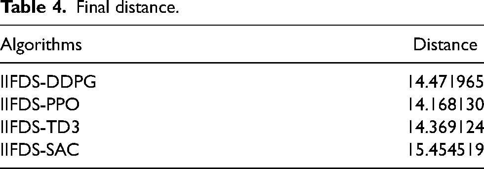
It can be seen that IIFDS-PPO is more stable than the other algorithms, and IIFDS-SAC is not as effective as the previous three algorithms in variable speed dynamic multi-obstacle environments, and the reason for this is that the SAC algorithm is not very good at the task of training the optimal near-edge actions.

Algorithmic advantages

To demonstrate that the IIFDS-DRL algorithm is indeed superior in path planning, we compare the algorithm with three traditional path planning algorithms. Traditional algorithms often fail to reach target points in the presence of unknown currents and dynamic obstacles. To compare their performance, various static obstacle environments were established. The IIFDS-DDPG algorithm was chosen as the variant of IIFDS-DRL with a larger discrete dispersion.

The experimental conditions were consistent across the four algorithms, with results displayed in Figure 11. The traditional methods selected for this study include the A* algorithm, ant colony optimization (ACO), and the RRT algorithm. The A* algorithm extends Dijkstra's approach to identify the least costly path between two vertices in a graph, allowing traversal through various connected nodes, each with an associated edge cost. The Ant Colony algorithm, introduced by Marco Dorigo in 1992 in his PhD thesis, is a probabilistic method that finds optimized paths by mimicking the behavior of ants searching for food. Ants preferentially select paths with higher pheromone levels, creating a positive feedback loop. Meanwhile, the RRT algorithm is widely utilized in robotic motion planning, focusing on generating viable paths by randomly sampling and effectively exploring the environment.

Figure 11.

Performance comparison between IIFDS and conventional algorithms.

The final distances of the four algorithms are shown in Table 5. The experimental comparisons clearly demonstrate that the algorithm proposed in this paper significantly outperforms traditional algorithms such as A*, RRT, and ACO in the domain of path planning. In various complex environments, the proposed algorithm in this paper consistently exhibits higher efficiency and superior path-planning capabilities.

Table 5.

Final distance.

Algorithms	Distance
A* algorithm	16.253243
Ant colony algorithm	29.712967
RRT algorithm	24.927685
IIFDS-DDPG	15.581810

Ocean current impact tests

Although ocean currents vary greatly in time and space across the vast ocean, their flow velocity and direction are relatively stable within certain specific sea areas. A stream function is defined to model non-circulating but time-varying ocean currents in these regions. ²⁶

$$\phi (\mathrm{x},\mathrm{y},\mathrm{t})=1\text{-}\tanh \left({\displaystyle \frac{\mathrm{y}\text{-}\mathrm{A}(\mathrm{t})\cos (\mathrm{k}(\mathrm{x}\text{-}\mathrm{ct}))}{{(1+{\lambda }^2\mathrm{A}(\mathrm{t}{)}^2{\sin }^2(\mathrm{k}(\mathrm{x}\text{-}\mathrm{ct})))}^{0.5}}}\right)$$

(25)

$$\mathrm{A}(\mathrm{t})={\mathrm{A}}_0+\alpha \cos ({\mathrm{w}}_0\mathrm{t}+\varphi )$$

(26)

Then the velocity of the ocean flow can be $(\text{-}\frac{\mathrm{\partial }\phi }{\mathrm{\partial }\mathrm{y}},\frac{\mathrm{\partial }\phi }{\mathrm{\partial }\mathrm{x}})$ , and the parameters are set as $\mathrm{k}=1,\mathrm{c}=0.12,\lambda =0.84,$ ${\mathrm{A}}_0=0.12,\alpha =0.3,{\mathrm{w}}_0=0.4$ . ²⁷

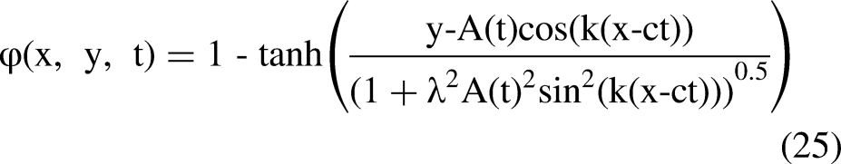
A spatial complex cyclic eddy is also established for path planning simulation studies. The current velocity in grid (x, y) is represented by $(\mathrm{u}(\mathrm{x},\mathrm{y}),\mathrm{v}(\mathrm{x},\mathrm{y}))$ described in equations (27) and (28).

$$\mathrm{u}(\mathrm{x},\mathrm{y})={\mathrm{U}}_{\mathrm{m}}\cos (\mathrm{x}\text{-}\phi )\sin (\mathrm{y}\text{-}\phi )$$

(27)

$$\mathrm{v}(\mathrm{x},\mathrm{y})=\text{-}{\mathrm{V}}_{\mathrm{m}}\sin (\mathrm{x}\text{-}\phi )\cos (\mathrm{y}\text{-}\phi )$$

(28)

Adding the modelled ocean currents to the multi-dynamic obstacle environment affects the AUV both horizontally and vertically. The IIFDS-PPO algorithm is used as an example to test the effect of ocean currents on the reward value. PPOC stands for the IIFDS-PPO algorithm with the influence of random ocean currents in the environment, and PPO stands for the IIFDS-PPO algorithm without the influence of ocean currents. The rest of the conditions of the two are the same except the ocean currents, and the results are shown in Figure 12. Influenced by the ocean currents on the motion, the IIFDS-PPO algorithm is never able to reach the next target point of the predetermined Q value in the previous rounds, which leads to a low reward value, and as the number of training times increases, the AUV gradually adapts to the environment of the random ocean currents, and the reward value is gradually recovered.

Figure 12.

Ocean current impact tests.

Conclusion

In this paper, we present IIFDS-DRL, an AUV path-planning method that incorporates the effects of stochastic currents. First, we build a simulated underwater environment containing dynamic obstacles and then test it using IIFDS combined with four common deep reinforcement learning algorithms. The results demonstrate the superiority of the method. The ocean current information gives the IIFDS-DRL algorithm intelligence, and the multiple training of deep reinforcement learning gives the algorithm stability, which makes the AUV reach the target point accurately and quickly. However, there are still some problems, regarding the energy consumption of the AUV and the more complex situations in the real world are still issues to be investigated and overcome.