Learning to drive as humans do: Reinforcement learning for autonomous navigation

Abstract

This article introduces an approach aimed at enabling self-driving cars to emulate human-learned driving behavior. We propose a method where the navigation challenge of autonomous vehicles, from starting to ending positions, is framed as a series of decision-making problems encountered in various states negating the requirement for high-precision maps and routing systems. Utilizing high-quality images and sensor-derived state information, we design rewards to guide an agent’s movement from the initial to the final destination. The soft actor-critic algorithm is employed to learn the optimal policy from the interaction between the agent and the environment, informed by these states and rewards. In an innovative approach, we apply the variational autoencoder technique to extract latent vectors from high-quality images, reconstructing a new state space with vehicle state vectors. This method reduces hardware requirements and enhances training efficiency and task success rates. Simulation tests conducted in the CARLA simulator demonstrate the superiority of our method over others. It enhances the intelligence of autonomous vehicles without the need for intermediate processes such as target detection, while concurrently reducing the hardware footprint, even though it may not perform as well as the currently available mature techniques.

Introduction

Autonomous driving ¹ has garnered significant interest from both the academic community and industry stakeholders, owing to its potential to transform mobility and transportation systems fundamentally. The SAEJ3016 standard ² categorizes motor vehicles into six levels of automation, ranging from Level 0 (L0) to Level 5 (L5), and defines the corresponding provisions for road motor vehicles as follows:

• L0:

No automation: The driver maintains full control of the vehicle while potentially receiving warnings or supplementary information.

L1:

Driver assistance: The vehicle performs closed-loop control for either steering or longitudinal acceleration/deceleration, with the driver managing other aspects.

L2:

Partial automation: The vehicle uses environmental perception data to execute closed-loop control over steering, acceleration, and deceleration, with the driver handling remaining tasks.

L3:

Conditional automation: The autonomous driving system assumes all driving operations, with human intervention only upon system request.

L4:

High automation: The motorized driving system performs all driving tasks, but within certain road and functional constraints.

L5:

Full automation: The autonomous driving system is capable of handling any driving conditions without human intervention.

Conventional autonomous driving planning and navigation methodologies are based on a modular data flow approach.^3–5 This approach comprises modules such as perception, positioning, planning and navigation control (PNC), remote control, and computer interaction. The data flow and communication between these modules are depicted in Figure 1. The PNC module is further divided into path planning, decision-making, motion planning, and motion control. While the modular approach simplifies the development of individual modules by breaking down complex driving tasks, it is prone to error propagation. For instance, in 2016, a Tesla vehicle’s perception module incorrectly identified a white tractor-trailer as a cloud, with tragic consequences. Moreover, the modular system’s demand for computational resources can lead to inadequate memory allocation for the PNC module, resulting in redundant computations and inefficient memory usage. These systems struggle with complex scenarios and often resort to discretization into finite-dimensional state machines, which may yield different decisions based on varying behavioral criteria. Overall, the majority of existing approaches concentrate on formal logic that delineates driving behavior within annotated three-dimensional geometric maps. This methodology can be challenging to scale effectively because it depends extensively on external mapping infrastructure, rather than primarily relying on an comprehension of the immediate surroundings.

Figure 1.

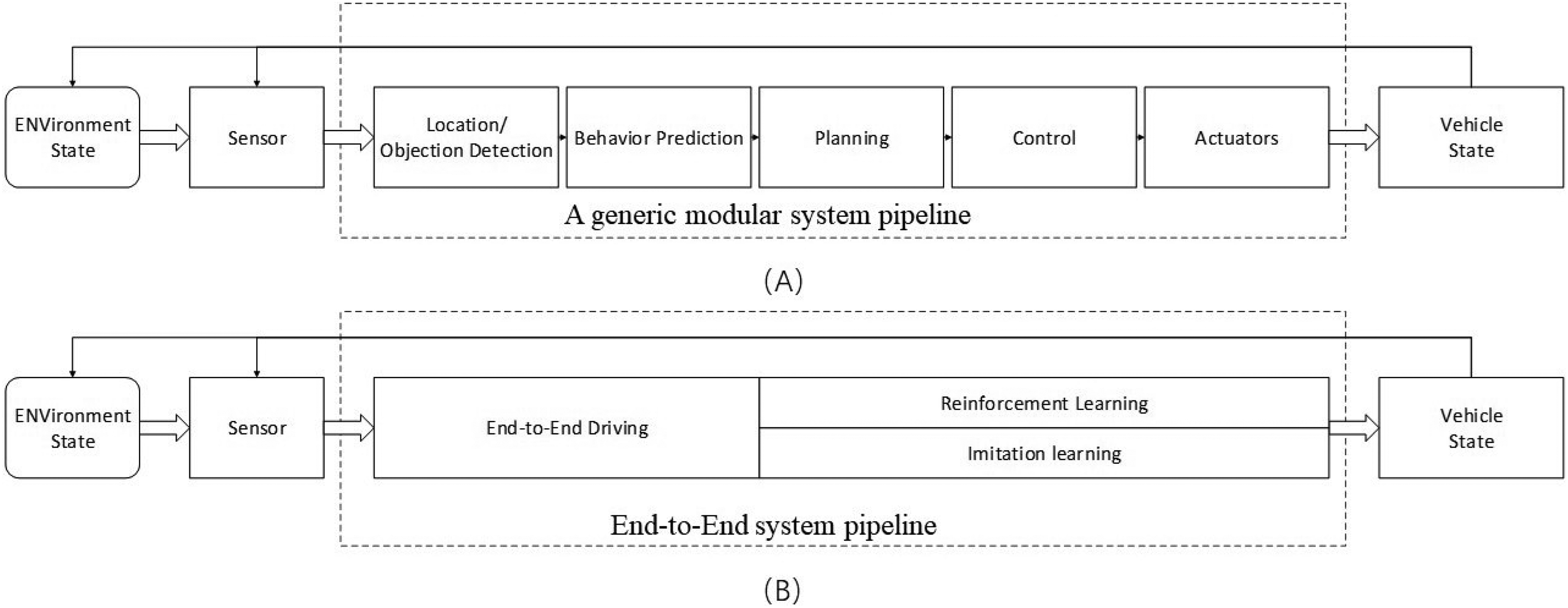
(A) A typical modular system pipeline, encompassing location or object detection, behavior prediction, planning, control, and actuators and (B) an end-to-end system pipeline focusing on reinforcement learning and imitation learning.

In reality, the scenarios encountered by autonomous vehicles are myriad and cannot be adequately captured by state machines. Encountering unforeseen situations can lead to confusion within autonomous driving systems. Furthermore, end-to-end systems offer an alternative approach to PNC, directly producing ego-motion from sensory inputs. Ego-motion can manifest as continuous actions of the steering wheel and throttle or as discrete actions such as acceleration or turning.

The end-to-end approach commences with data and learns behavior logic through imitation learning or self-learning, obviating the need for the vehicle’s dynamic model. The primary components of the end-to-end system include two learning methodologies: the imitation learning method based on supervised learning and the reinforcement learning method. Imitation learning extracts decision-making logic from expert data; however, its effectiveness is limited when faced with conditions not present in the expert dataset. Consequently, the behavioral logic of autonomous driving systems may not surpass the capabilities of human expert decision-making. Both traditional methods and imitation learning are constrained by human-centric thinking and are unable to transcend the bounds of human reasoning frameworks.

The autonomous driving system is conceptualized as an agent that employs reinforcement learning techniques. ⁶ The agent engages with the environment, garnering rewards in response to its actions. Its primary goal is to maximize cumulative rewards. By carefully designing incentives, we can align the objectives of autonomous driving with those learned through reinforcement learning, a process that mirrors human learning. Human drivers initially lack familiarity with a vehicle and learn through trial and error to identify the safest and most comfortable driving methods. They experience satisfaction upon mastering new skills or discovering new routes and guilt when causing accidents—these emotional responses are akin to the positive and negative rewards in reinforcement learning. The agent’s learning process, grounded in this concept, has the potential to exceed human learning capabilities. While driving, individuals can identify appropriate routes without depending on high-precision maps and navigation systems. In this article, we leverage reinforcement learning to facilitate autonomous driving navigation from the initial position to the termination point, negating the requirement for high-precision maps and routing systems.

This article introduces an approach aimed at enabling self-driving cars to learn to drive akin to human cognition. We implement the soft actor-critic (SAC) algorithm for planning and navigation from an initial to a termination position in autonomous driving negating the requirement for high-precision maps and routing systems. Our input is a multimodal state space, which includes high-quality images captured by cameras and state vectors comprising easily obtainable sensor data, such as speed and position. This multimodal state space provides the agent with a comprehensive understanding of the environment.

We leverage the variational autoencoder (VAE) algorithm to derive latent vectors from high-quality images, reusing them in place of the original images. This innovation addresses the drawbacks associated with the use of high-quality images, such as high memory usage, slow training speeds, and reduced training efficiency. Our method demonstrates superior performance in the CARLA simulation environment when compared to other approaches. Although it lags behind commercially available methods, it holds significant promise for autonomous learning and decision-making in autonomous driving. By utilizing high-quality images, we enhance the algorithm’s ability to garner information about the surroundings, facilitating migration from simulation to real-world environments.

The primary contribution of this research lies in proposing a novel method for autonomous driving planning and navigation negating the requirement for high-precision maps and routing systems that learns from scratch in a manner analogous to human drivers. This work establishes a foundational framework for the integration of true artificial intelligence in autonomous driving. By interpreting the planning and navigation task from a decision intelligence perspective, we enhance the autonomy of driving systems. However, our approach requires further development for application across all scenarios.

The remaining structure of this article is organized as follows: The “Related work” section on related work reviews the application and research status of reinforcement learning in autonomous driving and vehicle simulation environments. The “Deep reinforcement learning (DRL)” section details the principles of reinforcement learning algorithms, while the “Variational autoencoder (VAE)” section explains the VAE algorithm. In the “Components” section, we discuss the main components of reinforcement learning and VAE, along with their implementation. The “Experiments” section presents our method’s experimentation within the CARLA simulation environment and an analysis of the results. Finally, the “Conclusion” section summarizes the article and offers insights into potential future research directions.

Related works

In their 2021 paper published in Nature, Sutton and David Silver proposed that reinforcement learning could be applied in any domain where rewards are adequately designed. ⁷ While this perspective has sparked debate, primarily due to the complexity of reward design, it provides a theoretical basis for using reinforcement learning to achieve planning and navigation in autonomous driving systems that emulate human-like decision-making. Wayve, a UK-based startup, has focused on intensive learning for autonomous driving. In their 2020 study, ”Learn to Drive in a Day,” ⁸ they employed the deep deterministic policy gradient (DDPG) algorithm for autonomous lane-keeping. Initially, the authors used pre-trained agents within a simulator and later applied the pre-trained algorithms to physical vehicles for continued training on highways, using the distance traveled within a lane as a reward. The results indicated that the lane-keeping task could be achieved after approximately one hour of training on actual roads. Despite extensive research in reinforcement learning by scholars, there remains a scarcity of practitioners due to the challenges associated with convergence in the training process.

The process of continuous trial and error in practical training is scientifically unsound. This presents a significant challenge for researchers attempting to learn environmental models through offline reinforcement learning ⁹ and data collected from real-world vehicles. The discrepancy arises because the model is often a simulation environment derived from a constructor’s simulator, which can lead systems to equate the virtual world with the real environment.

To address this issue, the research community has adopted generative adversarial network theory, integrating an environmental discrimination process into the rendering phase to maximize the loss function between the real and rendered environments. In alignment with this principle, the Stanford team introduced the Gibson simulation environment in 2018,^10,11 primarily utilized in indoor mobile robotics. Additionally, Zhou et al. ¹² proposed the SMART simulation framework to simulate complex interactions among multiple autonomous vehicles, although it focuses on cooperative multi-agent interactions rather than providing detailed environmental information for individual agents, which is inadequate for our experimental requirements.

Although not tested on actual vehicles, we aimed for the highest possible accuracy in the virtual environment. We explored various simulation environments. The SMART simulator, ¹² developed by Huawei, emphasizes multi-intelligence collaborative training; the Gazebo simulation ¹³ is geared towards indoor robotics but lacks realism; the Gibson simulation, ¹⁰ designed by Stanford, is centered on indoor robotic interactions but does not represent an urban environment; likewise, the donkeycar simulation, ¹⁴ created by MIT, also does not simulate urban settings. The CARLA simulation environment ¹⁵ stands out by offering realistic urban conditions with a diverse fleet of car models, enabling Sim2Real transitions.

Despite advancements in simulation environments, preliminary research in reinforcement learning for PNC remains essential. ¹⁶ For instance, Chae et al. ¹⁷ employed the deep Q-network (DQN) algorithm to interpret sensor data for navigating complex obstacle scenarios, automatically assessing collision risks, and implementing autonomous braking for safe and comfortable driving. Isele et al. ¹⁸ used DRL to safely navigate through unsignaled intersections, outperforming traditional heuristic methods and demonstrating active obstacle avoidance.

Wang et al. ¹⁹ applied Q-learning to enable a vehicle agent to adapt its behavior for intelligent lane changing under various conditions. Sallab et al. ²⁰ utilized DQN and deep deterministic actor-critic to simulate lane-keeping in TORCS and to master autonomous maneuvering in complex curvature and interactive driving situations.

Current literature suggests that end-to-end planning and navigation modules in PNC research receive limited attention, primarily due to the novelty of reinforcement learning in autonomous driving and the scarcity of completed projects. An autonomous driving environment is significantly larger in scale compared to other agent simulations. To enhance the agent’s understanding of its surroundings, the state space incorporates both image data from cameras and a state vector containing vehicle speed, position, and other relevant data. We designed a reward function to facilitate autonomous navigation from an initial to a final destination negating the requirement for high-precision maps and routing systems.

Deep reinforcement learning

Reinforcement learning mimics one of the ways humans acquire knowledge and skills. DRL builds upon the principles of traditional reinforcement learning. ²¹ It leverages deep neural networks to approximate value functions and policy functions more effectively. Unlike traditional reinforcement learning methods that rely on linear functions and tabular representations to estimate these functions, as illustrated in Figure 2, DRL is particularly useful in scenarios such as autonomous driving, where the state space is too vast to be enumerated. In complex environments, the relationship between state and value spaces is inherently nonlinear, rendering simple linear approximations inadequate. Deep neural networks excel in capturing the underlying complexities of such relationships due to their high representational power.

Figure 2.

(A) The interaction between an agent and its environment and (B) the reinforcement learning process. The use of a neural network facilitates the approximation of the policy or value functions.

Deep Q-network

The DQN algorithm^22,23 represents a foundational value-based approach in which only the value function is employed to assess the quality of state-action pairs. It is an extension of Q-learning into continuous and high-dimensional spaces. In reinforcement learning, the state-action value $Q(s,a)$ denotes the expected cumulative discounted reward obtained from taking action a in state s until the terminal state is reached. $Q_{\pi }(s,a)$ refers to the value of following policy $\pi$ by taking action a in state s. The following equation formalizes this concept:

$$\begin{array}{rl}{Q}_{\pi }(s,a)& =\mathbb{E}[G_t|S_t=s,A_t=a]\\ & =\mathbb{E}\left[{\displaystyle \sum _{k=0}^{\mathrm{\infty }}{\gamma }^k{r}_{t+k+1}|S_t=s,A_t=a}\right]\end{array}$$

(1)

Here, $r(s_t,a_t)$ represents the reward obtained in state $s_t$ after performing action $a_t$ , and $\gamma$ is the discount factor. In traditional Q-learning, a Q-table maintains a one-to-one mapping between $Q(s,a)$ and $(s,a)$ pairs. When the transition probabilities and the value model are known, dynamic programming can be applied to calculate future rewards and subsequent states. However, in most cases, these probabilities and values are unknown, and the Bellman equation is used to estimate the state-action value at the next time step through bootstrapping, as shown in the following update rule:

$$Q(s,a)\leftarrow Q(s,a)+\alpha [r+\gamma \underset{a^{\prime }}{max}Q(s^{\prime },a^{\prime })-Q(s,a)]$$

(2)

This update rule is at the core of the DQN’s iterative improvement and its ability to learn effective policies in complex environments.

Where r represents the current reward, $\gamma$ is the discount factor, $s^{\prime }$ denotes the next state, and $a^{\prime }$ the subsequent action. In a finite-dimensional space, the table method serves adequately for estimating requirements. However, in the infinite-dimensional space pertinent to autonomous driving, we must resort to function approximation. Specifically, the construction of the function $Q_{\varphi }$ approximates the value function $Q_{\pi }$ , which we term value function approximation: $Q_{\varphi }\approx Q_{\pi }$ .

In value-based approaches, a critic assesses the efficacy of behaviors. The ultimate policy ${\pi }^{\prime }$ is derived by selecting actions according to ${\pi }^{\prime }(s)=\underset{a}{\arg max}{Q}_{\pi }(s,a)$ after fitting the Q-function. Consequently, the Q value informs the final policy. DQN employ a target network, where $Q_{\pi }(s_t,a_t)=r_t+\gamma Q_{\pi }(s_{t+1},a_{t+1})$ . To align the current policy with the target policy, DQN establishes a mean squared error (MSE) Bellman residual function.

In DQN, the policy is entirely contingent on the Q-function. For a given state, DQN iterates over all potential actions within the action space, selecting the one with the highest Q-value. These state-action pairs underpin DQN’s implicit deterministic policy. The $ϵ$ -greedy strategy addresses DQN’s exploration challenge, with a probability of $1-ϵ$ choosing actions based on the Q-function, while $ϵ$ allows for random exploration. Typically, $ϵ$ is set to a small value, such as $10\mathrm{\%}$ , ensuring that $90\mathrm{\%}$ of the time, actions are guided by the Q-function.

Experience replay mitigates data correlation by introducing a replay buffer. This buffer captures data through interactions with the environment under a specific policy $\pi$ . Subsequently, the stored data is used to update the Q-function, highlighting the off-policy nature of the algorithm; the policy being updated differs from the one used to collect the data.

Deep deterministic policy gradient

The DDPG algorithm, as described by Silver et al., ²⁴ concurrently learns the Q-function and the policy using off-policy data and the Bellman equation. It maintains consistency with the optimal action-value function, $a*=\underset{a}{\arg max}Q*(s,a)$ . In DDPG, a deterministic policy, $a_t=\mu (s_t)$ , is adopted, establishing a unique mapping between states and actions, typically represented by a policy function. This approach is particularly advantageous in environments with continuous action spaces.

For finite-dimensional discrete spaces, one can calculate and compare Q values for each action to determine the optimal policy. However, this enumeration is infeasible in infinite-dimensional continuous spaces. DDPG addresses this by optimizing the Q-function, which is differentiable with respect to the action space, thereby rendering the policy $\mu (s)$ differentiable with respect to the state. The Q-function’s gradient with respect to the state is expressed as $\underset{a}{max}Q(s,a)\approx Q(s,\mu (s))$ .

DDPG utilizes deep neural networks to construct the Q-function and employs a MSE loss function to approximate the current and target networks, thus refining the Q-function’s estimation. The neural network primarily consists of parameters $\theta$ , which are estimated to complete the network’s training. The network is updated using Polyak averaging, as represented by the update rule ${\theta }_{targ}\leftarrow \mathrm{polyak}{\theta }_{targ}+(1-\mathrm{polyak})\theta$ .

DDPG also employs neural networks for policy network estimation, as discussed by Sutton et al. ²⁵ The target policy network is instrumental in approximating the maximization problem associated with $Q_{targ}$ , and its parameters are subjected to Polyak averaging during the training process.

Twin delayed DDPG (TD3)

The DDPG algorithm is known for its sensitivity to hyperparameter tuning and can exhibit instability in its learning process. A common issue in DDPG is the Q-function’s tendency to overestimate Q-values, which can lead to the degradation of the learned policy. In contrast, TD3 addresses this by simultaneously learning two Q-functions, $Q_1$ and $Q_2$ , which minimize the mean squared Bellman error (MSBE). This approach is analogous to DDPG’s method of learning a single Q-function, with both Q-functions sharing a common objective. The target value is calculated using the smaller of the two Q-functions:

$$y(r,s^{\mathrm{\prime }})=r+\gamma \underset{i=1,2}{min}{Q}_{{\varphi }_{i,\text{targ}}}(s^{\mathrm{\prime }},a^{\mathrm{\prime }}(s^{\mathrm{\prime }}))$$

(3)

This strategy of targeting the smaller Q-value estimate helps prevent overestimation. In TD3, the Q functions are updated twice per iteration, while the policy function is updated only once. To further mitigate overestimation, TD3 introduces noise to the target action, making it more challenging for the policy to exploit the Q-function. This target policy smoothing acts as a regularizer that counters a specific failure mode in DDPG, where a Q-function’s sudden incorrect spike can lead to brittle or incorrect policy behavior.

The Q-learning target’s actions are derived from the target policy ${\mu }_{{\varphi }_{\text{targ}}}$ , with added clipped noise to each action dimension to smooth the Q-function across similar actions, which is the objective of policy smoothing. This noise is clipped to ensure the target action remains within the effective range of actions. TD3, like DDPG, trains deterministic policies in an off-policy manner, requiring agents to explore a sufficient variety of actions to discern valuable reward signals. This exploration is facilitated by adding uncorrelated Gaussian noise to the actions during training.

Soft actor-critic

SAC is an off-policy algorithm that optimizes stochastic policies. A key aspect of SAC is entropy regularization, which encourages the policy to balance the trade-off between expected returns and policy randomness, or entropy. This entropy term is closely tied to the exploration-exploitation trade-off: higher entropy promotes exploration, potentially accelerating learning, and helps prevent the policy from converging prematurely to suboptimal solutions.

The entropy H of a random variable x with probability mass or density function P is defined as follows:

$$H(P)=\underset{x\sim P}{\mathbb{E}}[-\log P(x)]$$

(4)

In SAC, the agent receives a reward that includes the policy’s entropy at each time step, altering the reinforcement learning problem to the following equation:

$${\pi }^{*}=\arg \underset{\pi }{max}\underset{\tau \sim \pi }{\mathbb{E}}\left[\sum _{t=0}^{\mathrm{\infty }}{\gamma }^t(r_t+\alpha H(\pi (\cdot |s_t)))\right]$$

(5)

Here, $\alpha >0$ is the temperature coefficient, which adjusts the relative importance of entropy in the optimization. Consequently, the action-value function $Q_{\pi }$ is redefined to incorporate this entropy term.

$$\begin{array}{rl}& Q^{\pi }(s,a)\\ & =\underset{\tau \sim \pi }{\mathbb{E}}[\sum _{t=0}^{\mathrm{\infty }}{\gamma }^t{r}_t+\alpha \sum _{t=1}^{\mathrm{\infty }}{\gamma }^{t}H(\pi (\cdot \mid s_t))\mid s_0=s,a_0=a]\end{array}$$

(6)

The recursive Bellman equation for the entropy-regularized $Q_{\pi }$ is as follows:

$$\begin{array}{rl}{Q}^{\pi }(s,a)& ={\mathbb{E}}_{s^{\mathrm{\prime }}\sim P,a^{\mathrm{\prime }}\sim \pi }[r+\gamma (Q^{\pi }(s^{\mathrm{\prime }},a^{\mathrm{\prime }})+\alpha H(\pi (.\mid s^{\mathrm{\prime }})))]\\ & ={\mathbb{E}}_{s^{\mathrm{\prime }}\sim P,a^{\mathrm{\prime }}\sim \pi }[r+\gamma (Q^{\pi }(s^{\mathrm{\prime }},a^{\mathrm{\prime }})-\alpha \log \pi (a^{\mathrm{\prime }}\mid s^{\mathrm{\prime }}))]\end{array}$$

(7)

The SAC algorithm simultaneously learns a policy ${\pi }_{\varphi }$ and two Q-functions $Q_{{\theta }_1}$ and $Q_{{\theta }_2}$ . Similar to TD3, it employs the clipped double-Q trick, where both Q-functions are trained by minimizing the MSBE:

$$\begin{array}{rl}L({\varphi }_i,\mathcal{D})& =\mathbb{E}\left[{(Q_{\theta }(s,a)-y(r,s^{\mathrm{\prime }},d))}^2\right]\\ y(r,s^{\mathrm{\prime }})& =r+\gamma (\underset{j=1,2}{min}{Q}_{{\theta }_{\text{target},j}}(s^{\mathrm{\prime }},{\hat{a}}^{\mathrm{\prime }})-\alpha \log {\pi }_{\varphi }({\hat{a}}^{\mathrm{\prime }}\mid s^{\mathrm{\prime }}))\\ {\hat{a}}^{\mathrm{\prime }}& \sim {\pi }_{\varphi }(.\mid s^{\mathrm{\prime }})\end{array}$$

(8)

Ultimately, the parameters across the networks are updated by backpropagating through the loss function, facilitating the learning of the policy from the collected data.

Variational autoencoder

The VAE^26,27 is fundamentally a method for density estimation based on latent variables. Although network design is not the primary focus in reinforcement learning, this article introduces an approach that utilizes high-quality images as inputs. High-quality images contain richer details compared to standard images commonly used in reinforcement learning tests. However, these images are larger in size, making them challenging for simple models to process. Moreover, it is impractical to input raw, high-resolution images directly into a system due to excessive memory requirements, which would limit the batch size during the training process of reinforcement learning algorithms. In this work, we employ a VAE to extract a latent vector from the original image, which is then used by the system to approximate the original image. The VAE estimates the parameters of a Gaussian mixture distribution using the expectation-maximization algorithm, with the primary objective being to maximize the probability $P(x)$ .

$$\begin{array}{rl}P(X)& =\frac{P(X,Z)}{P(Z|X)}\\ & \Rightarrow \log P(X)=\log P(X,Z)-\log P(Z|X)\\ & \Rightarrow \log P(X)=\log \frac{P(X,Z)}{q(Z)}-\log \frac{P(Z|X)}{q(Z)}\\ & \Rightarrow {\displaystyle \int q(Z)\log P(X)dZ}\\ & ={\displaystyle \int q(Z)\log \frac{P(X,Z)}{q(Z)}dZ-{\displaystyle \int q(Z)\log \frac{P(Z|X)}{q(Z)}dZ}}\\ & \Rightarrow \log P(X)\\ & ={\displaystyle \int q(Z)\log \frac{P(X,Z)}{q(Z)}dZ+{\displaystyle \int q(Z)\log \frac{P(Z|X)}{q(Z)}dZ}}\end{array}$$

(9)

Here, $P(X)$ denotes the probability distribution of the sample X, and $q(Z)$ represents a variational distribution. Consequently

$$\begin{array}{rl}\text{ELBO}& ={\displaystyle \int q(Z)\log \frac{P(X,Z)}{q(Z)}dZ}\\ KL(q(Z)\Vert P(Z|X))& ={\displaystyle \int q(Z)\log \frac{P(Z|X)}{q(Z)}dZ}\end{array}$$

(10)

The $\log P(X)$ can be decomposed into two components: the ELBO (evidence lower bound) and $KL(q(Z)\Vert P(Z|X))$ . If $q(Z)=P(Z|X)$ , then $KL(q(Z)\Vert P(Z|X))=0$ , and $\log P(X)=\text{ELBO}$ . Therefore, maximizing the ELBO is equivalent to maximizing $P(X)$ .

$$\begin{array}{rl}\text{ELBO}& ={\displaystyle \int q(Z)\log \frac{P(X,Z)}{q(Z)}dZ}\\ & ={\displaystyle \int q(Z)\log P(X,Z)dZ-{\displaystyle \int q(Z)\log q(Z)dZ}}\\ & ={\mathbb{E}}_{Z\sim q(Z)}[\log P(X,Z)]-{\displaystyle \int q(Z)\log q(Z)dZ}\end{array}$$

(11)

In this expression, $\int q(Z)\log q(Z)dZ$ is a constant term. Maximizing the expectation of $\log P(X,Z)$ is the objective. However, while $P(Z|X)$ is typically tractable, we cannot directly set $q(Z)=P(Z|X)$ to make $KL(q(Z)\Vert P(Z|X))=0$ . Variational inference is employed to approximate $q(Z)$ as $q(Z|X)$ :

$$\begin{array}{rl}\log P(X)& ={\displaystyle \int q(Z|X)\log \frac{P(X,Z)}{q(Z|X)}dZ}\\ & +{\displaystyle \int q(Z|X)\log \frac{P(Z|X)}{q(Z|X)}dZ}\\ \Rightarrow \log P(X)& ={\displaystyle \int q(Z|X)\log \frac{P(X|Z)P(Z)}{q(Z|X)}dZ}\\ & +KL(q(Z|X)\Vert P(Z|X))\\ \Rightarrow \log P(X)& ={\displaystyle \int q(Z|X)\log P(X|Z)dZ}\\ & +{\displaystyle \int q(Z|X)\log \frac{P(Z)}{q(Z|X)}dZ+KL(q(Z|X)\Vert P(Z|X))}\\ \text{with}\text{ELBO}& ={\displaystyle \int q(Z|X)\log P(X|Z)dZ}\\ & -{\displaystyle \int q(Z|X)\log q(Z|X)dZ+{\displaystyle \int q(Z|X)\log P(Z)dZ}}\\ \text{ELBO}& ={\displaystyle \int q(Z|X)\log P(X|Z)dZ-KL(q(Z|X)\Vert P(Z))}\end{array}$$

(12)

Upon optimizing the bundle of latent expected objectives (ELBO), the KL-divergence, $q(Z|X)\Vert P(Z|X)$ , is concurrently minimized. Presuming that a mixture of Gaussian distributions can adequately approximate any intricate probability function for continuous latent variables Z, the vector feature z is extracted from the input distribution by the VAE as a representation of the latent space.

Components

This section delineates the modular constituents integral to the reinforcement learning process within the context of autonomous driving navigation negating the requirement for high-precision maps and routing systems, including the state space, action space, and policy network. Furthermore, it elucidates the training procedures for both the VAE and the reinforcement learning algorithm.

Environment

The agent engages with the environment, where it acquires the current state $s_t$ and reward $r_t$ . It formulates decisions based on these parameters and executes the corresponding action $a_t$ . This action impacts the environment, leading to the generation of the subsequent state $s_{t+1}$ . OpenAI-Gym ²⁸ provides a generic framework for reinforcement learning environments, characterized by its reset and step functions. The reset function initializes the state, offering the agent an initial state $s_0$ , while the step function processes the agent’s action and yields a reward, the next state, and an indicator of termination, done.

In our research, the CARLA simulation environment is employed to emulate autonomous driving through urban landscapes. CARLA operates on a service-client architecture, necessitating the scripting of a client to facilitate network communication with the service and create a reinforcement learning environment. For our experiments, we utilize the TownHD10 map from CARLA, within which we establish a world with a physical town. We determine a starting point for the vehicle and a destination for navigation on the map. The objective is for the vehicle to autonomously traverse from the starting point to the designated destination negating the requirement for high-precision maps and routing systems.

As depicted in Figure 3, the Neolix autonomous logistics vehicle is equipped with a variety of sensors, including lidar, camera, collision sensors, an inertial measurement unit (IMU), and ultrasonic sensors. ²⁹ In our setup, we employ only a visual sensor—a camera with a 60-degree field of view—to perceive the vehicle’s surroundings. Additionally, we incorporate a collision sensor to detect any collisions. The vehicle operates freely within the town, receiving real-time decisions from the agent. Training rounds conclude upon collision, and navigation is considered successful when the vehicle’s position is within one meter of the target position, at which point the termination state done is set to true.

Figure 3.

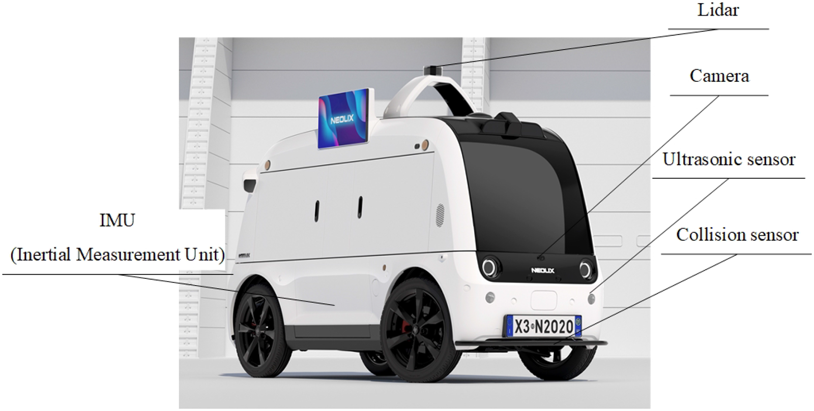
The Neolix unmanned logistics vehicle is fitted with sensors such as lidar, camera, collision sensors, inertial measurement unit (IMU), and ultrasonic sensors.

Reward design

In reinforcement learning, the reward serves as the sole feedback from the environment to the agent, assessing the quality of the current state. Compared to supervised learning, the limited information provided by the reward makes the training process of reinforcement learning more gradual and challenging. The design of the reward mechanism is crucial in guiding the agent towards decisions that align with the objectives of the task. A significant challenge in reinforcement learning is determining whether the reward design is sufficient to steer the agent’s behavior in accordance with the intended goals. The design of reward mechanisms is often shaped by our profound familiarity with a given domain. In order to enhance the agent’s experiential learning, a reward system that integrates both dense and discrete rewards is implemented, instead of the traditional terminal state reward at the end of each episode. This is a solitary, sparse reward granted upon success or failure. Many scholars argue that learning is made more arduous due, in part, to the paucity of rewards associated with effort. Often, the impact of such meager rewards is not immediately realized. For instance, in the game of Go, the reward is only bestowed upon the determination of a winner between two players at the end of the game, with negative feedback being the sole indicator of reward, its timing in player evaluation remaining ambiguous.

In reward system design, a distinction is drawn between sparse and dense rewards. Dense rewards are provided at every frame. Initially, to motivate the vehicle to proceed, we define $r_{distance}$ as the distance the vehicle has traversed. To deter the vehicle from moving backward, we employ the difference in distance between consecutive frames as the reward, as opposed to the raw distance. The potential energy reward is a function of the distance between the vehicle and the destination, with positive rewards for approaching the destination and negative otherwise—all of which are classified as dense rewards. Additionally, to hasten the vehicle’s arrival at the destination and ensure it maintains a speed above a specified threshold, we introduce $r_{velocity}=v-v_{set}$ , where v is the current speed of the vehicle and $v_{set}$ is the minimum required speed. The reward $r_{velocity}$ is positive if the vehicle exceeds this speed and negative if it falls below.

To prevent the vehicle from idling and generating an abundance of irrelevant data, we have implemented an additional dense reward, $r_{timeout}$ . If the vehicle’s speed remains at $0m/s$ for 100 steps, the episode is terminated and a negative reward of $-1$ is given. To avoid collisions, the environment inflicts a negative reward $rewar{d}_{collision}$ upon the agent when a collision is detected. Conversely, a positive reward $r_{success}$ is granted when the vehicle successfully reaches the target position.

Upon collision or successful arrival at the destination, the episode concludes, and the vehicle reverts to the starting point to initiate a new data collection cycle. While the agent is theoretically motivated to pursue positive rewards and avoid negative ones, empirical observations suggest that the reward values should be tightly controlled. Excessive positive rewards can lead to an overestimation of the value function. Hence, it is crucial to constrain rewards within a specific range to preclude outliers that could skew the learning process. The rewards are aggregated according to their weighted coefficients:

$$\begin{array}{rl}reward& =c_1{r}_{distance}+c_2{r}_{velocity}\\ & +c_3{r}_{timeout}+c_4{r}_{collision}+c_5{r}_{success}\end{array}$$

(13)

Here, $c_1\sim c_5$ represent the weighted coefficients for each reward type.

State space

The state is derived directly from the visual sensor of a camera, and policies are generated from the raw image data. In considering the image size, we opt for a lower resolution that is resource-efficient, such as 64 by 64 pixels. The capacity of humans to extract meaningful features from these small images is overlooked, despite the reduced resource consumption and accelerated training pace that they offer. Smaller images inherently result in the loss of certain features. While humans may discern between two images based on nuanced details, these may be irrelevant for our purposes.

For example, the orientation of a pedestrian’s palm at an intersection might indicate their intended direction of travel, yet such granular details are not always pertinent. Low-resolution images may fail to capture such nuances, making high-resolution images more suitable for training decision-making algorithms. Utilizing high-resolution images as states not only facilitates the translation of our algorithms to real-world applications but also aids in the sim2real transfer learning process.

Nonetheless, a significant challenge arises with the use of large images. These images not only consume substantial memory but also lengthen the time required for model updates, potentially compromising the algorithm’s effectiveness. To maintain the intricacies of high-resolution images while simultaneously minimizing their memory footprint, an asynchronous training approach is a promising method. In this scheme, Process 1 is tasked with data collection, while Process 2 is dedicated to model training. These processes communicate through dedicated pipes, facilitating concurrent interaction with the environment and agent updates. This reduces the update latency and enhances training efficiency. Concurrently, the collected data is stored offline on a hard drive, with each frame’s information archived independently. However, we found that while this strategy mitigates memory usage, it fails to address GPU memory consumption. An excessive $batch\mathrm{\_}size$ during training can lead to program termination and crashes. To address this, we employ a VAE ³⁰ to derive latent vectors from high-quality images, ensuring that the system perceives these vectors as consistent with the original images. These latent vectors serve as a proxy for the underlying state.

The VAE provides a simplified representation of the image, utilizing the vehicle’s state information to generate an autonomous state vector that includes data such as speed and distance. This data is derived from the vehicle’s internal sensors, such as the IMU and odometer. By integrating the image state matrix, which correlates with speed, with a state vector containing acceleration, we construct the agent’s state space.

Action space

Reinforcement learning algorithms such as DDPG, TD3, and SAC are commonly applied to action spaces with a potentially infinite number of dimensions. ³¹ In the context of autonomous driving, the actions under our control are limited to acceleration, braking, steering, and gear shifting. For simplicity, we exclude the shifting action, precluding the agent from reversing the vehicle. CARLA provides a control interface with $throttle,brakes\in [0,1]$ , and $steering\in [-1,1]$ . Since applying the brake and accelerator simultaneously is impractical, we merge the brake and throttle into a single dimension, where $brakeandthrottle\in [-1,1]$ . This allows for a more natural and efficient control scheme, with $[-1,0]$ representing deceleration and $[0,1]$ representing acceleration.

The selected actions mirror those taken by human drivers, resulting in a two-dimensional action space: $[-1,1]$ for the combined throttle and brake, and $[-1,1]$ for steering. Empirical observations suggest that extreme acceleration and steering angles are unnecessary. By adjusting the control parameters, such as the difference between the accelerator and the brake, we can align them more closely with the throttle range. This refinement not only accelerates training but also prevents the agent from fixating on the braking action, which could generate an abundance of superfluous data.

Replay buffer

To facilitate the interaction between the agent and the environment, a five-dimensional tuple $<s_t,a_t,r_t,s_{t+1},done>$ is recorded. Here, $s_t$ denotes the current state, $a_t$ the current action, $r_t$ the reward obtained by transitioning from the current state to the next via the current action, $s_{t+1}$ the subsequent state, and done a flag indicating whether the current state is terminal, encoded as true or false. Reinforcement learning employs a replay buffer mechanism ³² to decorrelate samples. This buffer stores the experienced tuples, and during training, random sampling is performed to reduce data similarity. While caching data in memory is expedient for basic experiments with limited data volume and dependencies, this approach is not always suitable for more complex experimental setups aimed at evaluating algorithmic performance.

To mitigate the challenge of excessive memory usage, we employed a dual-pronged approach. First, we established an offline localized replay buffer, as exemplified by Fu et al., ⁹ which serves as both the training and test datasets for the VAE. Specifically, we localized the data, storing each data tuple in the h5py format as an individual file. This method facilitates the creation of an offline localized replay buffer.

For the task of autonomous driving navigation, we selected an off-policy algorithm. The key difference between on-policy and off-policy algorithms lies in whether the policies employed for evaluation or improvement are identical to those generating the sampled data. This allows us to leverage offline data to refine and update the policy. However, during experimentation, we encountered a persistent issue of file corruption due to concurrent read-write operations over the same data file. Although our innovative use of the offline localized replay buffer effectively addressed the issue of large memory consumption, this approach was not fully compatible with the reinforcement learning training process. File locking could lead to process interlocks, resulting in a wait state that is inconsistent with the demands of parallel asynchronous training. Additionally, the import of large images could lead to excessive GPU memory usage, compromising training effectiveness and potentially causing crashes.

We redefine the state post-VAE processing of the original image as the latent state. Consequently, the original five-dimensional tuple $<s_t,a_t,r_t,s_{t+1},done>$ is reconstituted as $<\mathit{\text{latent}}{s}_t,a_t,r_t,\mathit{\text{latent}}{s}_{t+1},done>$ . We then reconstruct a novel replay buffer, termed the latent replay buffer, using this new tuple, effectively addressing the issue of large image memory occupation.

VAE training

We apply VAE to high-quality images to derive the corresponding latent vectors. This process allows us to reduce the dimensionality of the images while retaining their essential features. Utilizing a random policy to control the vehicle’s movement within the environment, we store the generated data from each frame in h5py files via offline localization. Each file contains a 5-tuple of data. The collected data is preserved within an offline localized replay buffer of size 32768, from which the VAE samples data to train its model.

As depicted in Figure 4, the VAE’s network structure comprises two sub-networks. The left sub-network is the Encoder, responsible for fitting $q(Z|X)$ , while the right sub-network is the decoder, which fits $P(X|Z)$ . We approximate these models using deep neural networks. The encoder consists of a convolutional neural network (CNN) and a multilayer perceptron. It takes a high-quality image input of 640 $\times$ 640 pixels. The CNN’s initial hidden layer applies 32 4 $\times$ 4 filters with a stride of 2, followed by a rectified linear unit. Successive hidden layers apply 64, 128, 256, and 32 filters, each with the same configuration and activation function. We flatten the output to pass through the bottleneck, which is divided into mean and variance networks, to obtain the latent vector. The decoder, a deconvolutional network, inverts the encoding process by upsampling the latent vector to match the size of the input image.

Figure 4.

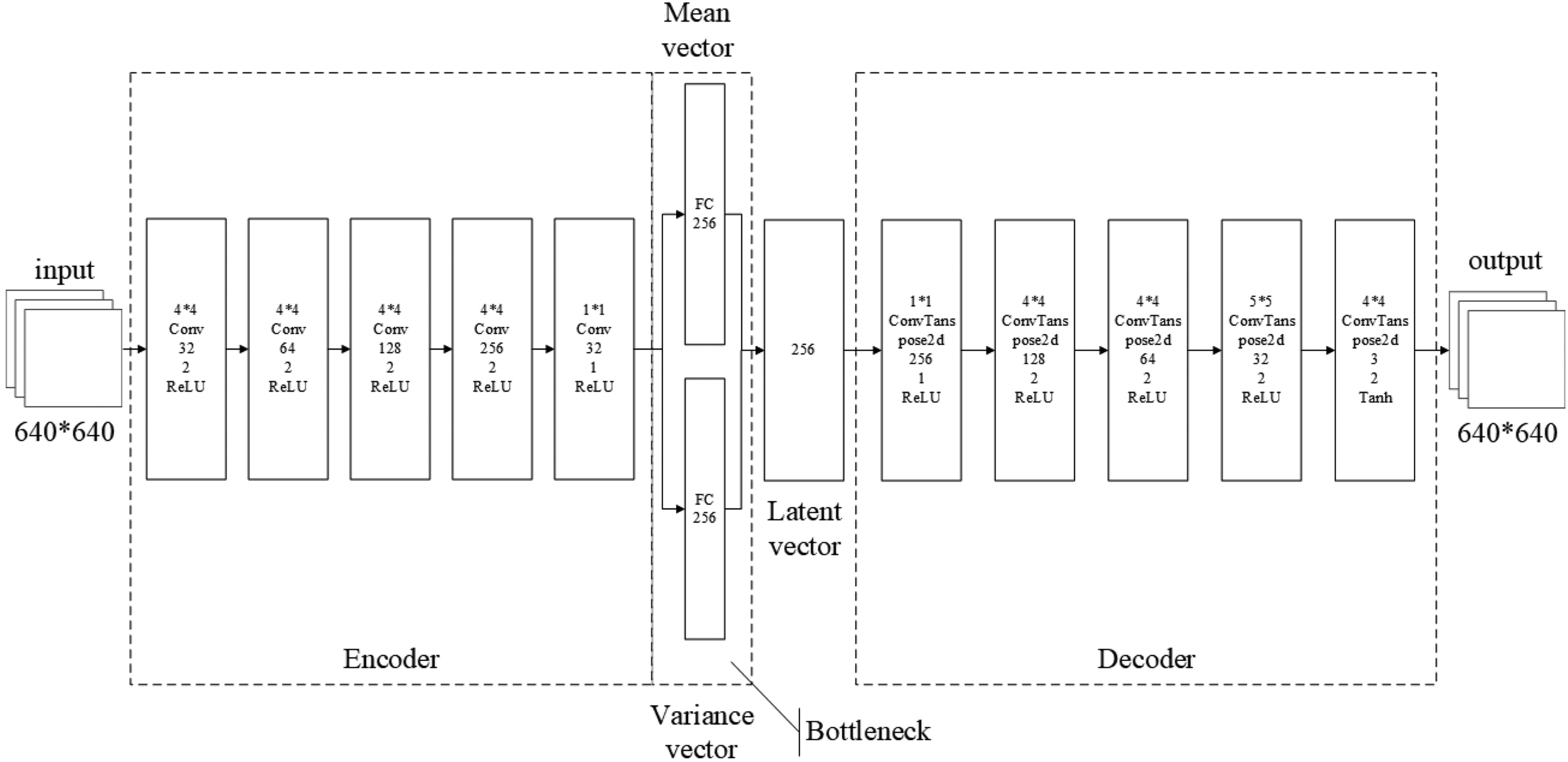
The architecture of the variational autoencoders (VAE) consists of two components: the encoder and the decoder. The mean and variance networks are employed to approximate the distribution of the latent vector.

We sampled a dataset $\{X_1,X_2,\dots ,X_n\}$ from the offline localization replay buffer. We computed the posterior probability $q(Z_n|X_n)$ of each sample with respect to the latent variable through the encoder. Subsequently, we randomly sampled a vector Z from the posterior distribution and fed it to the decoder to generate the reconstructed data $\{{\hat{X}}_1,{\hat{X}}_2,\dots ,{\hat{X}}_n\}$ . For training, we selected the visual state $s_t$ from the offline localized replay buffer, achieving the desired results after 500,000 training iterations, as depicted in Figure 5. Our objective was for $q(Z_n|X_n)$ to be better aligned with the distribution $P(Z)$ and for the reconstructed data $\{{\hat{X}}_1,{\hat{X}}_2,\dots ,{\hat{X}}_n\}$ to closely resemble the original dataset $\{X_1,X_2,\dots ,X_n\}$ within the VAE framework. We aimed to maximize the ELBO, which is equivalent to minimizing the negative ELBO:

$$-\text{ELBO}=-\int q(Z|X)\log P(X|Z)dZ+\text{KL}(q(Z|X)\Vert P(Z))$$

(14)

Figure 5.

(A) An image captured by a camera placed in the CARLA environment for autonomous driving and (B) The processed image by the encoder and decoder modules of the variational autoencoders (VAE).

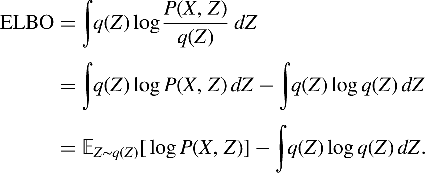
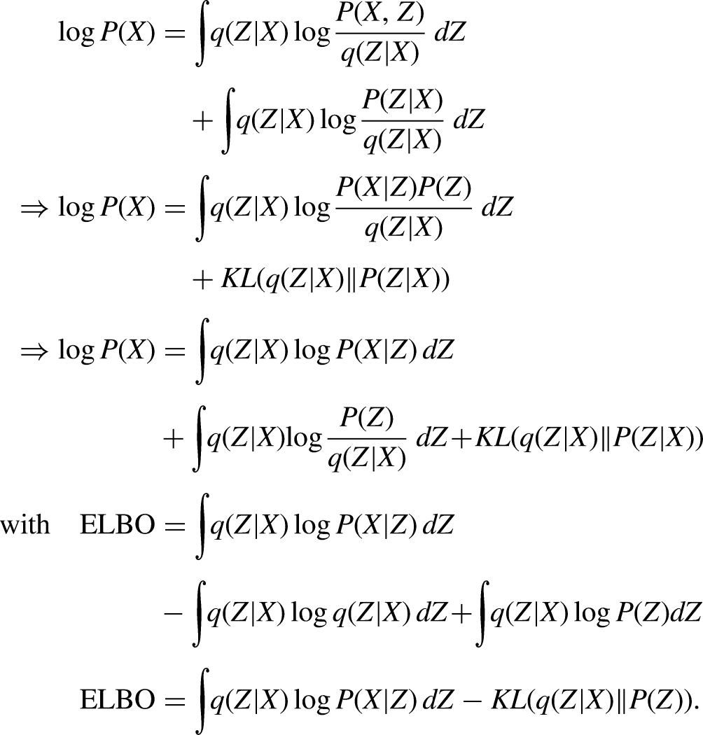
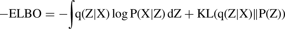
We decomposed the negative ELBO into two terms: the first term corresponds to the reconstruction loss, while the second represents the KL divergence. These serve as the loss functions for the encoder and decoder, respectively. We sought to minimize the sum of these two losses. Optimization was performed using stochastic gradient descent, with the network optimization process being equivalent to parameter estimation.

Reinforcement learning training

We developed an Agent to simulate vehicle driving within the CARLA environment. This Agent can represent either a human driver or an autonomous control system. The autonomous driving task was carried out in a town scenario simulated by CARLA, with the policy function $a={\mu }_{\theta }(s)$ and value function $q=Q_{\varphi }(s,a)$ being updated based on the observed state and reward. We approximated these functions using neural networks, given that DDPG, TD3, and SAC are similar off-policy reinforcement learning algorithms. The policy and value network frameworks were designed to be generalizable. The inclusion of the latent state significantly simplified the network structure.

To enhance the richness of the state representation, we adopted a multi-modal state space. This included the latent state processed by the VAE and a vector state comprising multiple intrinsic states. We processed each modality separately using MLPs to generate 128-dimensional tensor vectors. These vectors were concatenated to form a new 256-dimensional tensor, which constituted the feature extraction layer. The output from this layer was used as input for three subsequent fully connected layers, with ReLU activation functions applied between them. The fully connected layers contained 256, 32, and four neurons, respectively.

In reinforcement learning, the actor network, as depicted in Figure 7, refers to the policy network, while the critic network, as shown in Figure 6, corresponds to the value network. Although these networks share an identical architecture, their distinct input and output characteristics reflect their differing objectives. The critic network receives state and action pairs as inputs and outputs the corresponding Q-values. Conversely, the actor network takes the state as input and produces either the distribution over actions or the actions themselves. It is imperative to train both networks simultaneously to enhance the critic’s ability to assess the policy and to enable the actor to derive a superior policy. Consequently, the parameters of these networks diverge.

Figure 6.

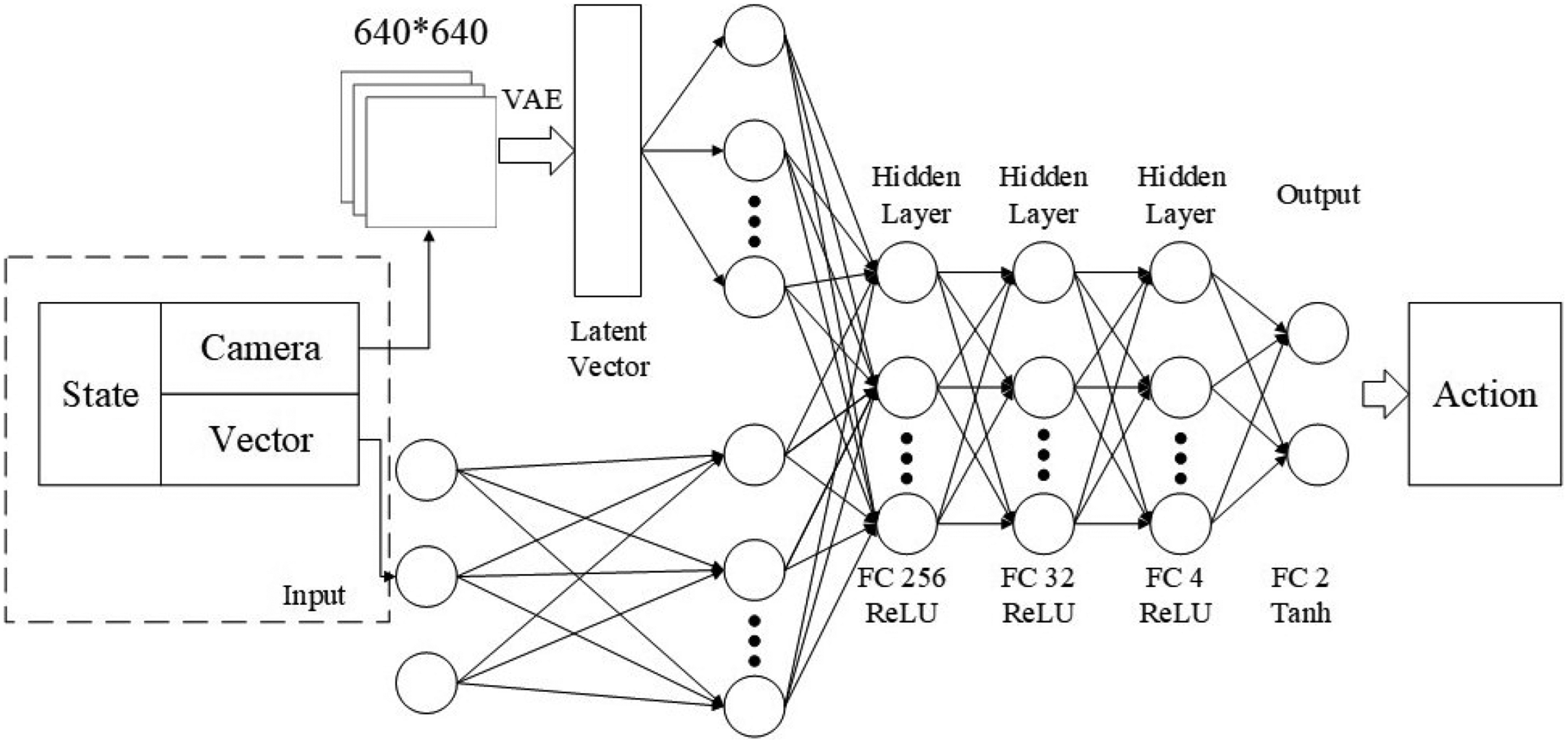
The actor-network: this network approximates the policy function using a neural network. It accepts states as inputs and yields actions or action distributions as outputs.

Figure 7.

The critic network: this network employs a neural network to approximate the value function. It takes state and action pairs as inputs and produces Q-values as outputs. These Q-values are used to evaluate the quality of the policy.

Experiments

Conducting experiments in a real-world setting presents significant challenges. Locating an appropriate experimental site for autonomous driving and equipping it with autonomous vehicles capable of autonomous navigation negating the requirement for high-precision maps and routing systems is a complex task. Autonomous vehicles rely on images and other sensors to collect data about their environment, amassing relevant information during their operations. This data encompasses sensor information and environmental rewards for autonomous behavior. The process of driving autonomously involves continually refining the policy through trial and error until the optimal policy is discovered, allowing the vehicle to execute its tasks effectively. Achieving the optimal policy requires numerous updates, which can span more than a day. Furthermore, reinitializing the autonomous vehicle to its starting position at the beginning of each episode demands considerable time and effort. The frequent failures during trial-and-error training are unnecessary and unreasonable in the context of autonomous driving.

To address these challenges, we replicate the experimental environment within a simulation platform, as described in the “Environment” section. We construct a simulation environment on the CARLA platform that mirrors the real-world environment, leveraging the unreal engine for rendering. This simulation closely approximates the real environment, both visually and in terms of the system’s interactions. By using a simulation, we eliminate concerns over labor costs and potential vehicle damage. The simulation platform is established on a server running Ubuntu 20.04, equipped with an NVIDIA RTX 3090 graphics card, which supports model training and image rendering with its 24 GB of memory. The simulation environment is configured as depicted in Figure 8(A). It simulates a cityscape, complete with residential and commercial buildings, wide roads, traffic signals, and vehicles. For the purposes of this experiment, we choose to disregard traffic signals and regulations. Figure 8 illustrates the overall map of the environment, with point A serving as the starting position and point B as the destination.

Figure 8.

(A) The TownHD10 scene within the CARLA environment in green, and (B) the corresponding map of TownHD10 in red.

We aim to enable autonomous vehicles to navigate from position A to position B negating the requirement for high-precision maps and routing systems. To this end, we employ the DDPG, TD3, and SAC algorithms for autonomous driving navigation. The experimental setting is based on the Town10HD map within the CARLA simulation environment. The weather conditions in this environment are characterized by clear skies, absence of wind, and represent a standard outdoor scenario. Comparative experiments were conducted in three stages. Initially, we ensured that all three algorithms utilized the same state input, and their image inputs were processed by an identical VAE model to obtain a consistent latent state representation.

Subsequently, each algorithm was subjected to the same number of update iterations and identical hyperparameters, as detailed in Table 1. This consistent setup facilitated a fair comparison among the algorithms.

Table 1.

Hyperparameters used in each algorithm for the experimental setup.

Hyperparameter	Value
buffer_size	65536
learn_rate	$1.00\times {10}^{-3}$
batch_size	100
Gamma	0.99
Tau	0.005

We evaluated the performance of the algorithms based on their success rate, mean episode length, and mean rewards, as presented in Figures 9 and Table 2. The success rate represents the proportion of successful episodes out of 200 trials. Mean episode length (mean_lens) denotes the average number of steps taken per episode, while mean_rewards indicates the average rewards accumulated over 200 episodes. “steps” refer to the number of training updates for the agent.

Figure 9.

Experimental result curves obtained by the three algorithms: (A) the mean_rewards curve for DDPG, TD3, and SAC algorithms; (B) the mean_lens curve; and (C) the success_rate curve. DDPG is represented by the red curve, SAC by the orange curve, and TD3 by the green curve. DDPG: deep deterministic policy gradient; TD3: twin delayed deep deterministic policy gradient; SAC: soft actor-critic.

Table 2.

Comparative results of the experiments for each algorithm, including DDPG, TD3, and four variations of SAC: SAC_1 trained at 1 million time steps, SAC_2 at 1.5 million, SAC_3 at 2 million, and SAC_4 with low-quality image state input. PNC refers to the traditional modular planning navigation method.

Algorithm	Training			Evaluation			Steps
	Mean reward	Success rate	Mean lens	Mean reward	Success rate	Mean lens
DDPG	9.893022537	0	200	−3.954	0	200	1.5M
TD3	20.76493263	0	200	−2.7314	0	200	1.5M
SAC_1	45.176	0.49	176	37.4948	0.726	183	1.0M
SAC_2	45.02	0.51	162	38.0278	0.746	178	1.5M
SAC_3	44.795	0.5	175	36.16	0.667	185	2M
SAC_4	21.986	0.01	196	0.371	0	200	1.5M
PNC	–	–	–	83	1	1113	–

DDPG: deep deterministic policy gradient; TD3: twin delayed deep deterministic policy gradient; SAC: soft actor-critic; PNC: perception, navigation, and control.

For the training process, DDPG, TD3, and SAC were all trained with the same hyperparameters as shown in Table 1. The red, green, and orange curves in Figure 9 represent the results of DDPG, TD3, and SAC, respectively.

In Figure 9(A), we compared the mean episode lengths of the three algorithms, which reflect the number of steps required to reach the end of each episode. We observed that DDPG and TD3 exhibited initial improvements, possibly due to a random policy at the early stages of the method selection. However, during the later stages of training, when faced with the same autonomous driving environment, these algorithms demonstrated similar performance. Their actions deviated in the later stages, often resulting in a loop of high-speed rotations and collisions, indicating a lack of effective policy learning.

Figure 9(B) reveals that the average rewards obtained by DDPG and TD3 tend to flatten out towards the end of training. In Figure 9(C), the success rates of the algorithms were compared, showing a success rate of zero for both DDPG and TD3. This indicates that these algorithms were unable to navigate from the initial to the final position in the designed environment.

From the comparisons in Figures 9(A) to (C), it is evident that the SAC algorithm significantly outperformed the others. The SAC algorithm appeared to successfully navigate from the starting point to the destination. SAC exhibited greater exploratory behavior than TD3 and DDPG. We identified biases in the action spaces of TD3 and DDPG and attempted to enhance their exploratory capabilities by adding random noise. However, these modifications did not overcome the significant deviations in training results, and the additional data collected did not contribute to improved policy learning.

In Table 2, the training phase is summarized through Figures 9 to 11. We have selected mean_rewards and success_rate as the key performance indicators for the algorithms.

Figure 10.

This figure presents the experimental result curves obtained from the application of three algorithms. We denote the soft actor-critic (SAC) algorithm trained for 1 million timesteps as SAC_1, depicted by the red curve; for 1.5 million timesteps as SAC_2, represented by the orange curve; and for 2 million timesteps as SAC_3, shown by the green curve: (A) the mean_lens curves for SAC_1, SAC_2, and SAC_3. (B) the mean_rewards curves, while (C) the success_rate curves for these algorithms.

Figure 11.

The depicted experimental result curves are the outcomes of two algorithms. SAC_1 represents the SAC algorithm with VAE, trained on high-quality images for 1 million timesteps, while SAC_4 signifies the SAC algorithm without VAE, trained on low-quality images for the same duration: (A) the mean lens curves for SAC_1 and SAC_4. (B) the mean rewards curves, and (C) the success rate curves for both algorithms. SAC: soft actor-critic; VAE: variational autoencoder.

We investigate how varying training durations might influence the experimental outcomes. As depicted in Figure 10, we employ three training durations: 1M, 1.5M, and 2M, which are denoted as SAC_1, SAC_2, and SAC_3, respectively. These algorithms are distinguished by the colors red, yellow, and green in the figure. We observe that training duration has a negligible impact on the mean_len and mean_rewards of the episodes shown in Figure 10(A) and (B). Figure 10(C) indicates that the success_rate was consistent in the initial stages of training and did not increase, but instead exhibited a sinusoidal pattern over time. Consequently, we conclude that extending the training duration is unlikely to enhance the success_rate.

In this study, we have consistently used high-quality images as inputs to extract a richer set of features. We employed VAEs to derive latent vectors from these images and construct a latent state space. We compared the efficacy of this state space with one utilizing $64\times 64$ low-quality images under the SAC algorithm. As depicted in Figure 11, the SAC method that uses the low-quality image input is labeled SAC_4 and represented by the blue curve. Figure 11(A) shows that the episode length for SAC_4 does not stabilize, suggesting that the autonomous vehicle is in a state of random exploration, potentially due to the limited information provided by the smaller image input. Despite having longer episode lengths, as shown in Figure 11(B), SAC_4 exhibits lower mean_rewards compared to SAC_1, indicating the significant advantage of high-quality images in enhancing algorithmic performance.

In the preceding paragraphs, we analyzed the algorithm by comparing training-phase parameter indicators. Subsequently, we evaluated the methods from the perspective of the evaluation phase, as presented in Table 2. Mean_rewards and success_rate were selected as algorithmic indicators. We employed the model saved after training for evaluation and testing purposes. In contrast to the training phase, the evaluation phase strategy is deterministic and lacks exploration. The model from the final training phase was tested 200 times to obtain mean_rewards and success_rate. Five rounds of testing were conducted to calculate an average. We observed that the success rate was significantly higher in the evaluation stage compared to the training stage when using SAC 1, SAC 2, and SAC 3. This is because, after model stabilization during training, the exploration process still introduces disturbances, increasing policy randomness. Furthermore, we found that SAC significantly outperformed both DDPG and TD3. The results indicate that increased training time does not necessarily lead to improved performance. The SAC algorithm with high-quality images as state input consistently outperformed its low-quality image counterpart in autonomous driving navigation tasks, demonstrating superior performance to DDPG and TD3. Our SAC algorithm successfully accomplishes autonomous driving navigation from start to finish in urban environments negating the requirement for high-precision maps and routing systems.

As depicted in the final row of Table 2, we have compared our proposed method with the traditional approach.

The traditional method, which is currently the most stability-deployed system in real vehicles (e.g. Dosovitskiy et al. ¹⁵ ), is referred to as planning navigation and control. According to the table, the PNC method exhibits the highest stability and success rate, which highlights the relative immaturity of our method. Additionally, the PNC method has the longest mean trajectory length, indicating that it requires the most time and that the trajectory planning module does not always generate the most optimal path. This underscores a limitation of the PNC approach, where errors in intermediate modules can affect the overall experimental outcomes.

Conclusion

We introduce a novel framework for autonomous driving planning and navigation, which endows autonomous vehicles with human-like driving capabilities. Our method utilizes reinforcement learning to enable autonomous navigation from initial to final destinations within urban settings negating the requirement for high-precision maps and routing systems, mimicking one of the ways humans learn to drive. Innovatively, we incorporate high-quality images and state vectors as multimodal inputs to learn policies from such imagery. Furthermore, we apply VAEs to address the memory-intensive requirements, low training efficiency, and complexity associated with high-quality images. Our method was tested in the CARLA simulation environment and demonstrated superior performance compared to other algorithms.

Although the success rate of our reinforcement learning-based autonomous navigation is lower than that of traditional methods, it is significant in the realm of autonomous learning and decision-making. The training process is particularly challenging due to the complexity of urban environments. Our approach relies solely on onboard cameras and sensors for environmental perception, eschewing the prior knowledge elements, such as lane markings and target recognition, used by traditional methods. This self-learning navigation technique has the potential to surpass human driving capabilities and is thus of profound importance.

In the context of autonomous driving agents, the current environment is complex, yet it remains straightforward for traditional methods and human drivers. This study establishes a foundation for future research, where we anticipate the application of reinforcement learning algorithms to achieve autonomous navigation in even more intricate settings. The existing reward function and state representation are not directly applicable to more complex environments. Therefore, we aim to enhance the generalizability and success rate of reinforcement learning algorithms in future research, primarily through improvements in reward design and state estimation.