
Abstract
In the multi-robot swarm control algorithm, the traditional rigid formation algorithm has low formation redundancy, and it is difficult to flexibly adapt to the external environment. In this study, centroidal Voronoi tessellation (CVT) was used to control a group of robots for forming the required flexible formations and increasing the structural redundancy and internal carrying capacity of the multi-robot system. When the CVT area is divided in a non-convex environment, the Voronoi and non-convex areas will overlap, which will cause the robot to collide with the obstacles and hinder the optimization of the cost function. In this study, constrained CVT was used to solve the problem of region overlap in non-convex environments. The proposed path planning algorithm ensured the safe movement of the robot and explored the applicability of the algorithm in different scenarios. Finally, the performance of the algorithm in the non-convex area was verified and discussed by analyzing the simulation and experimental results for the convex and non-convex environments. The results showed that the constrained CVT could control the robot to generate the formation as quickly as possible in the non-convex area, and it was easy to dynamically switch the formation according to the external environment.
Introduction
Swarm robotics has attracted wide attention in the field of intelligent control and has replaced humans in natural resource prospecting, forest fire monitoring, 1 spacecraft exploration, 2 multi-robot mapping, disaster relief, and other areas. Multi-robot formation control is an essential branch of multi-intelligent systems wherein multiple robots are required to maintain a particular formation and avoid collision during a mission. Over the years, extensive research results have been reported on multi-robot formation control and various formation control methods have been developed based on the leader–follower method, 3 behavior-based control method, 4 virtual structure method, 5 artificial potential field method, 6 and self-organizing coverage method based on gradient and grouping. 7 These formation methods have different advantages and disadvantages and are often used in combination to achieve the desired formation effect in various application scenarios. The advantage of the leader-following method is that the formation structure is simple and easy to implement, but the leader's mistake will be propagated through the entire system. The behavior- based method decomposes the robot motion into basic behaviors, but it cannot clearly define the overall behavior of the formation system, which is not conducive to the stability analysis of the system. The advantage of an artificial potential field is that it can enable the robot to avoid obstacles, but it can easily fall into local optimization. Nevertheless, it can reduce the system cost, improve the system's robustness and efficiency, and provide redundancy, reconfigurability, and structural decomposition for the system simultaneously.8,9
Formation control mostly aims for a fixed formation. All robots would implement their mission well even if they do not have to maintain the desired distance between them, provided they do not collide with each other. The centroidal Voronoi tessellation (CVT) algorithm used in this study ensures collision avoidance and facilitates the proper formation of multiple robots. 10 The CVT algorithm implements the distributed calculation to optimize the cost function by using a Voronoi partition. 11 Further, according to the properties of the Voronoi diagram, this method can ensure that the agents move only within their own Voronoi areas to avoid collisions. A careful review of the literature shows that most researchers have used this algorithm for dealing with robot swarm control in convex areas.12,13,14 Corte et al. 15 proposed a Voronoi partition and Lloyd's descent algorithms. It was assumed that the sensor moves according to the first-order dynamics. They proved that the sensor position converges to the Voronoi configuration of the center of mass, which is also the local optimal coverage for the cost function related to the sensing performance.
However, their algorithm cannot directly adapt to a non- convex environment with obstacles owing to the following two reasons. First, the sensing ability may be attenuated because of obstacles, thus invalidating the sensing model based on the Euclidean distance. Second, when the center of mass is outside the area, it cannot be guaranteed that the center of mass of the Voronoi area is set as the desired sensor target position.
In the case of robots with relatively simple functions in the swarm robot system, the limitations of computing power and communication load prevent them from adapting to a larger-scale complex task environment. Therefore, complex environments mainly have the following two challenges: how can swarm robots create a formation more flexibly and improve the internal robustness and flexibility to adapt to large-scale expansions? How can swarm robots adapt to a variety of non-convex environments of greater complexity to ensure the safety of the robots during their movements while maintaining their performance.
In response to the above challenges, this paper proposes a swarm control algorithm for a convex environment, and swarm control and path planning algorithms for a non-convex environment. It is ensured that the swarm robot system can adapt to a more complex non-convex environment while flexibly forming a swarm robot system. Simultaneously, it can optimize the cost function without reducing the performance of the swarm, and guarantee the safe movement and expansion ability of the swarm robots. The CVT-based swarm robot control can be applied to more practical scenes. These scenes are non-convex, it contains randomly distributed obstacles and holes.
The organization of this article is as follows. Section “State of the art” presents the state of the art. Section “CVT-based swarm control algorithm” presents the swarm control algorithm based on CVT. It then explains the difficulty in CVT tessellation in a non-convex environment, and describes the constrained CVT and path planning algorithm developed in this study. Subsequently, it presents the control law and related proofs. Section “Simulation of convex and non-convex areas” describes and analyzes the simulation experiments and results for different scenarios. Section “Swarm robotics experiment” presents the experimental results of this study. Finally, Section “Conclusion and future work” presents the conclusion and discusses the scope of future work.
State of the art
Most groundbreaking studies have considered only barrier-free environments. As is well known, the existing results for such an ideal environments are difficult to generalize to more complex obstacle areas. To overcome these limitations for a non-convex area, Boardman et al., 16 Prabowo1 et al., 17 and Collins et al. 18 solved the global coverage control problem of multirobots in a non-convex environment by combining the Voronoi tessellation and corresponding path planning algorithms. Among them, Prabowo et al. used the greedy best-first search algorithm to calculate the best center of mass outside the obstacle according to whether the center of mass is inside the obstacle to increase the coverage time performance. Although these methods are advantageous in terms of scalability and calculation time, they cannot guarantee the optimal trajectory of the robot, and the cost function converges slowly.
Stergiopoulos et al. 19 and Nair et al. 20 used the geodesic distance instead of the traditional Euclidean distance, allowing multiple robots to be deployed in a non-convex environment. However, it is difficult to avoid collisions when the center of mass and current position of the robot pass over obstacles. Finally, owing to the high cost of geodetic distance calculation, it is easy to cause the robot to fall into the extreme point owing to obstacles.
Aiming at the robot collision problem that may occur under the geodesic distance, Breitenmoser et al. 21 introduced the geodesic distance and combined the classic Lloyd algorithm with a local path planning algorithm, TangentBug, to calculate the robot's movement near obstacles and corners. The unreachable centroid is mapped to the reachable area, which proves the convergence and optimality of the algorithm. Palacios-Gasós et al. 22 realized the Voronoi tessellation in a non-convex area by utilizing the geodesic distance combined with the weighted Voronoi diagram. In addition, the coverage area scan of the non- convex area was realized through regional gridding and an online path planning algorithm.
Caicedo-Nunez et al. 23 and Xu et al. 24 mapped the connected regions in a class of non-convex environments to the convex regions through diffeomorphism and used the Lloyd algorithm to effectively solve the coverage problem in simple non-convex environments. However, this method is not effective in coverage problems under multiple obstacles or more complex non-convex environments.
Howard et al. et al. 25 proposed a combination of Voronoi tessellation and the potential field method. The robot is used as a virtual particle subject to make the robot and the obstacle repel each other so that multiple robots can cover the area to the greatest extent. On this basis, Renzaglia et al. 26 made the robot repel the obstacles while being attracted to the Voronoi centroid, thus completing the coverage of the robot in a non-convex environment.
Lu et al. 27 and Mahboubi et al. 28 defined a visibility- based Voronoi diagram based on the attenuation of sensor capabilities caused by boundary walls or obstacles. Among them, Lu et al. used the centroid projection method to solve the problem of the centroid lying outside the Voronoi region, and introduced smoothness constraints during the deployment process to avoid the phenomenon of sharp turns of the robot.
In addition, unmanned aerial vehicles (UAVs) are important in the research field of optimal coverage control. Some core features and control methods of UAVs and the related future work have been presented by Tahir et al. 29 Du et al. 30 reviewed the scheduling problem and expounded on the intelligent algorithm of the UAV swarm. They also discussed the constraints in various tasks. Chen et al. 31 applied swarm drones to agricultural applications such as spraying of pesticides. CVT was used to identify the best position of the drone during the spraying process, and its combination with the proposed intelligent health balance system extended the overall service life of the drone. In another research, Chen et al. 32 eliminated the toxic substance diffusion process through a set of statically connected grid sensor networks, which was modeled as a distributed parameter system controlled by parabolic partial differential equations. Govindaraju et al. 33 used drone swarming to monitor the forest and proposed a probabilistic sensor model to alleviate visibility degradation caused by vegetation. CVT was used to calculate the way points, and the linear combination of the terrain contour and vegetation cover was used as the density distribution function. By compromising on the average visibility, the strategy of pushing the observation points to dense vegetation areas can provide near-uniform visibility across the area. The strategy of pushing the observation points toward the local peak can provide higher average visibility across the entire area. CVT solved the problem of optimal planning of the movement trajectory of multiple UAVs in the air. However, the research was limited to the convex environment. As the areas in most practical application are non-convex, this largely limits the application of CVT-based swarm robots.
CVT-based swarm control algorithm
CVT swarm control
In the deffnition of the Voronoi tessellation algorithm, a region containing n generated points is partitioned into n cells. Each cell contains a generated point, and the other points in the cell are close to the generated point of that cell, thus ensuring that the cost function of the system reaches the minimum value. 34 CVT is a particular type of Voronoi tessellation, which sets the density function of the target region, and its generated point is the centroid of each Voronoi cell.
Suppose Q represents a convex polytope. A single robot in a multi-robot system has the position


CVT algorithm under constraints
According to the geometric shape, the task environment can be divided into convex and non-convex areas. If any two points in a certain area can be connected by a line segment that has no common point with the graph, then this area is called a convex area, as shown in Figure 1(a). The convex area is defined algebraically as shown below.

Task area classification. (a) Convex area. (b) Non-convex area.
In an area

In the Euclidean space, a convex set is a set of points in which the points on a straight line between every two points are included in the set of points. For convex areas, the controller based on the Lloyd algorithm can ensure that the generated points asymptotically converge to the centroid of their respective Voronoi areas, as shown in Figure 1(a). However, this result has some problems for non-convex areas. Figure 1(b) depicts the centroid position generated by the CVT algorithm at the initial time, but there is an obstacle (big black disk) between the robot (brown circle) and the target point (blue cross). This will lead to errors in the Euclidean distance calculation. Therefore, the CVT partition in a non-convex environment needs improvement.
To solve the problem of robot Voronoi tessellation in different areas under different density functions, the CVT algorithm calculates the position of the center of mass in each Voronoi cell. First, it is necessary to ensure that the Voronoi cells cannot contain obstacles inside the region.
Assuming that the Voronoi area corresponding to each robot in the swarm robotics is

After ensuring that each Voronoi cell is within the region, the resulting centroid position may appear outside the region,considering that the region is non-convex.Hence, the centroid position needs to be restricted.This is accomplished by strictly constraining the centroid of the Voronoi region within the Voronoi region, as shown in Eq. (11).

The target position and robot position relative to the obstacles are divided into the four cases shown in Figure 2.

Relationship between obstacles and paths.
The brown circle represents the current position of the robots, the blue cross represents the target position of the robots, the blue shaded area represents the obstacle, and the dotted line represents the safe path of the robots relative to the obstacle. The trajectory of the robot is marked with a red line. r is the radius of the obstacle, and
In Figure 2(a), the path between the robot and the target point does not pass through the obstacle, and the robot can directly track its target. At this time,
In Figure 2(b), the path between the robot and the target point is tangential to the obstacle; hence, the robot can still track the target directly, and
In Figure 2 (c), the straight path between the robot and the target point is blocked by the obstacle. The robot moves along the arc with radius R to avoid collision with the obstacle, and
In Figure 2 (d), the line between the robot and the target point passes through the center of the obstacle, that is,
Constrained CVT algorithm.

Proof of convergence
The robot control rate in CVT is expressed as


Simulation of convex and non-convex areas
Formation control in convex (obstacle-free) areas
The simulation experiments in this paper were performed on a MATLAB simulation platform with Windows OS. In MATLAB, the robot was assumed as a first-order dynamics model, and the specified area size was

Multi-robot square formation simulation. (a) Density function. (b) Square formation. (c) Position error. (d) Cost function value.

Multi-robot line formation simulation. (a1) Density function. (b) Square formation. (c) Position error. (d) Cost function value.

Initial positions of the robots in the multi-robot system.
The desired formation determined the value of the density function. For a square formation, the density function was initialized to a constant value of 1. As shown in Figure 3(a), when the initial density function in the region Q was constant, the region was partitioned using the Voronoi algorithm, and the robot tracked the location of the generated point to complete the square formation. The unit of each grid is 1 cm, and the lengths of the x-axis and y-axis are both 10 m. In Figure 3(b), the solid lines of different colors represent the robot's tracking trajectory.
In the initial phase of the experiment, the positions of the robots were randomly distributed near the origin, where the value of the cost function was the maximum. As the CVT algorithm was iterated, the generated point tended to move toward the centroid of each Voronoi cell, and the value of the cost function gradually decreased. When the generated points in the Voronoi cell reached their respective centroid positions, the cost function value was zero and the CVT algorithm converged, as shown in Figure 3(d). Figure 3(c) shows the position error between the robot and its corresponding centroid. At the beginning, the sum of the errors between the robots’ positions and the Voronoi generated points was the maximum. As the iterations of the CVT algorithm progressed, the error fluctuations gradually decreased owing to the PID controller, and the distance between the generated point and the centroid tended to the gradient descent. When the CVT algorithm converged, the error between the robots’ positions and the generated points eventually tended to zero.
Based on the density function as a constant, the line formation of the robots can be completed by adjusting the density function to a “V”-shaped function. The expression for the “V”-shaped function is shown in Eq. (10). The robots will remain in the high-density areas so that they can create the line formation. This density function distribution is shown in Figure 4(a), with a region size of 10 × 10 m2. The line formation is shown in Figure 4(b).
In the line formation process, the robots need to first complete the Voronoi partition under the constant density function distribution; hence, the cost function value at the initial moment is the maximum. During the iteration of the CVT algorithm, the controller overshoots due to integral saturation. The value of the cost function decreases significantly when the number of iterations is approximately 80. The optimal solution is reached again when the number of iterations is approximately 270, as shown in Figure 4(d). Figure 4(c) shows the position error between the robot and its corresponding centroid. As with the square formation, the robot's position error and the generated point are most significant during the initial stage of control. During the iteration of the CVT algorithm, the error fluctuation decreases gradually due to the gradient descent of the distance between the generated point and the centroid.
Non-convex (obstacle) swarm control
The task environment of swarm robotics usually contains irregular non-convex areas. For strictly convex areas, the Lloyd algorithm's controller can ensure that the generated points asymptotically converge to the centroid of their individual Voronoi cells. Unfortunately, this result is inapplicable to non-convex areas and convex areas with obstacles. As shown in Figure 6(a), ten points were randomly generated in a convex environment. Based on the Lloyd algorithm, the generated points finally converge to the centroid of their respective regions to obtain the distribution. It is assumed that there are circular obstacles in the environment and the area becomes non-convex. Under this condition, if the same method as in the convex environment is applied here, the center of mass will occur at the obstacle, as shown in Figure 6(b). This distribution method is unreasonable, as the robot can move only outside the obstacle, as shown in Figure 6(c).

Effect of obstacles on CVT. (a) Convex area. (b) CVT area over. (c) Non-convex area laps with obstacle.
To conclude, we consider that the following two fundamental issues must be satisfied to allow the use of swarm robotics in a non-convex environment:
(i) The divided Voronoi area cannot be within an obstacle; (ii) The center of mass of each Voronoi cell cannot be inside the obstacle.
Only by strictly limiting the position of the Voronoi cell and the center of mass can it be ensured that when the robot follows the corresponding center of mass to cover the environment, it remains inside the environment area.
A set of simulations was designed for the distribution of robots in a non-convex environment with different parameters. By adjusting the size, distribution, and number of obstacles, the influence of the obstacles on the value of the cost function was examined, and the effects of different parameters on the distribution efficiency of swarm robotics were observed to identify the most energy-efficient swarm control scheme. Furthermore, in order to determine the optimal number of robots, simulations were conducted with fixed obstacle sizes. By adjusting the number of robots, the impact of robot quantity on coverage rate and coverage efficiency was observed. The criterion for judging the stability of the swarm robotics is that the average value of the sum of errors between the position of each robot and its center of mass is less than 0.001, that is, the swarm reaches the target position.
Radius changes of obstacle
The time consumed, that is, the total iteration time, refers to the time required for the system to reach stability. In this study, the experiments were conducted with Microsoft Windows 10 operating system, Intel(R) Core (TM) i7-10750H, and 512 GB memory.
The sizes of the obstacles were changed to verify the performance of the algorithm proposed in this paper under obstacles of different sizes. The 10 × 10 environment was again used in this experiment. Figure 7(a), (b), (c), and (d) shows the final distributions of multiple robots for obstacles of different sizes when the obstacle center is at (5,5) and the radius r is 0, 1, 2, 3. The corresponding cost function is shown in Figure 8. The minimum values were obtained when the number of iterations was 124, 113, 82, and 102, respectively. It is considered that the swarm reached the stable state. The experimental data are shown in Table 2.

Different sizes of obstacles. (a) r = 0. (b) r = 1. (c) r = 2. (d) r = 3.
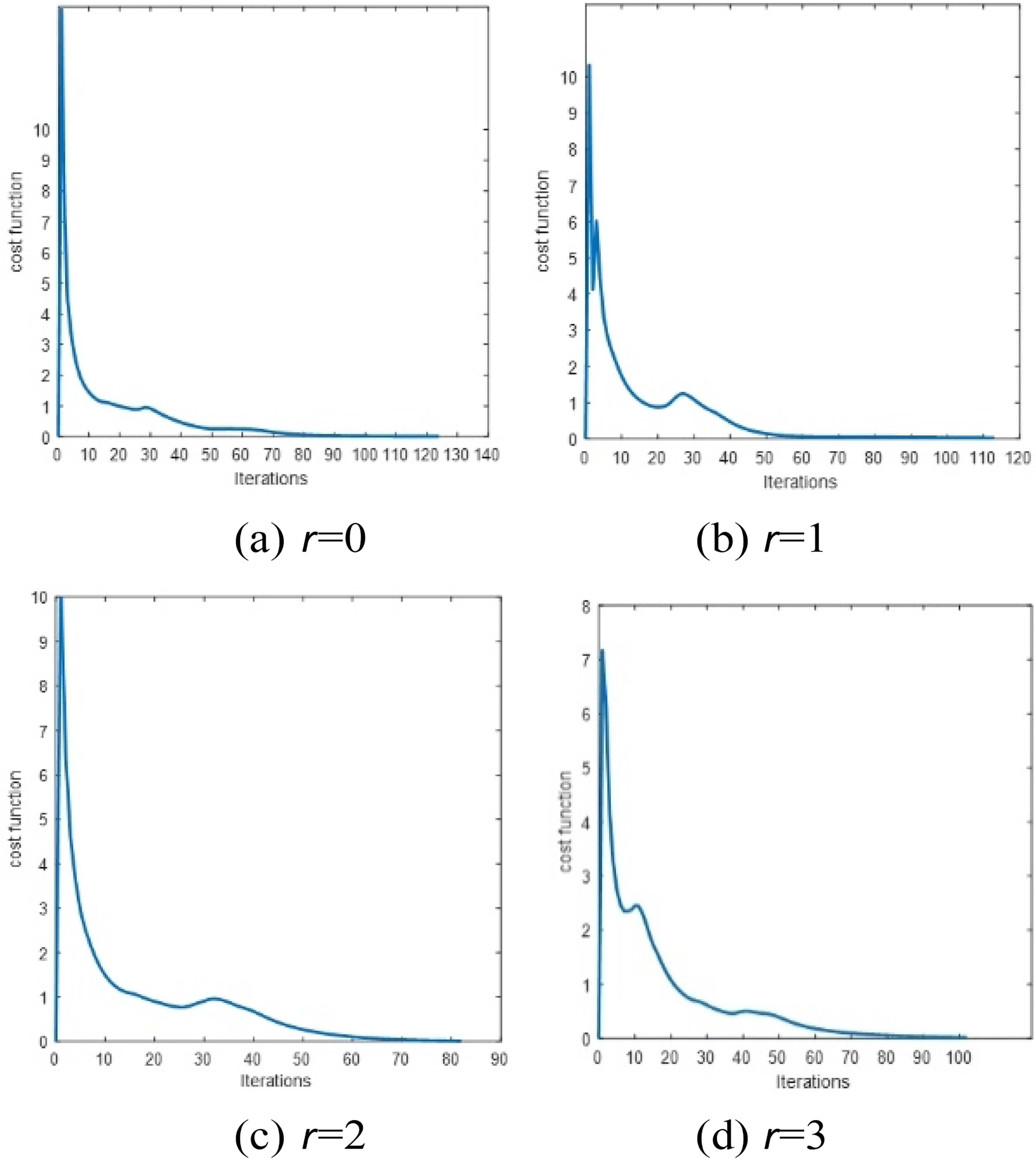
Cost function values for different sizes of obstacles. (a) r = 0. (b) r = 1. (c) r = 2. (d) r = 3.
Different size of obstacles.

From Figure 7 and Table 2, it can be seen that the size of the obstacle affects the degree of non-convexity of the environmental area. The algorithm can ensure a reasonable partition of the environment for obstacles of different sizes. However, a greater number of obstacles will increase the computation effort required for the algorithm. When the obstacle radius gradually increases, the area that the robot can effectively divide becomes increasingly smaller, which decreases the number of iterations and time in the steady state. When Different locations of obstacle
In the virtual environment, in addition to obstacles being of different sizes, their positions are usually random. The experiment reported here verified the effectiveness of the proposed algorithm when obstacles occur at different positions. The 10 × 10 environment was again used in this experiment. For

Different location of obstacles. (a) Position (3,3). (b) Position (5,5). (c) Position (7,7).

Cost function values for different obstacle locations. (a) Position (3,3). (b) Position (5,5). (c) Position (7,7).
Different location of obstacles.

Figure 9 and Table 3 show that the algorithm can ensure a reasonable partition of the area for different locations of an obstacle. Figure 10 shows the graphs of the cost function for different locations of the obstacle. The iterations were the smallest when the obstacle was located at the center of the area. When the obstacle was at (3,3), which was close to the robots, the partition conditions of the Voronoi cell were not maintained; hence, the algorithm recalculated the centroids of the Voronoi cell, which increased the computation cost. The robots moved in the opposite direction when the obstacle was at (7,7). The obstacle was encountered toward the end of the area. Therefore, the fluctuation was not apparent for a few iterations at the beginning. In the range of 20 to 30 iterations, the cost function fluctuated wildly but eventually stabilized. However, in these two cases, the robots overcame several situations where there were obstacles in the environment. When the obstacle was at (5,5), the iterations were smaller than in the other cases because the initial positions of the robots were significantly different from the desired locations. It can be seen that as the obstacle position moved closer to the center, the iteration time required was longer.
Different quantities of robots
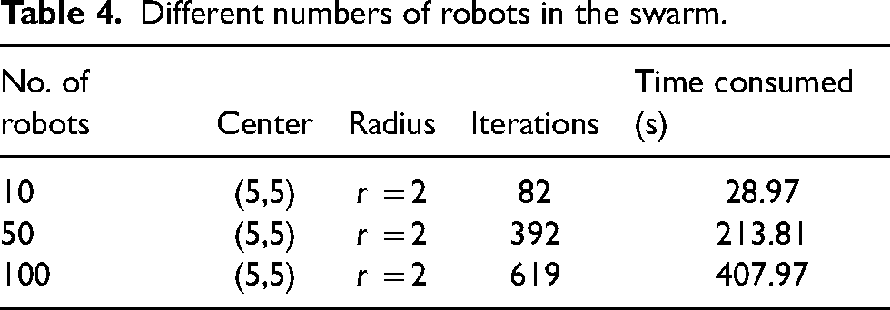
This section verifies the robustness of the algorithm to variation in the number of robots. Figure 11 shows a graph of the experimental results and Figure 12 shows the graphs of the cost function for different numbers of robots in the swarm. The minimum values were obtained when the number of iterations was 82, 392, and 619 for 10, 50, and 100 robots in the swarm, respectively.

CVT for different numbers of robots in the swarm. (a) n = 10. (b) n = 50. (c) n = 100.

Cost function value for different numbers of robots in the swarm. (a) n = 10. (b) n = 50. (c) n = 100.
Figure 11 and Table 4 show that the algorithm can ensure a profitable partition of the environment for different numbers of robots in the swarm. If the other parameters remain unchanged, as the number of robots increases, the amount of calculation inevitably increases, and the number of iterations required for system area stabilization will increase accordingly. It can be concluded that the greater the number of robots in the swarm, the greater will be the amount of calculation and iteration time.
Different quantities of obstacles
Different numbers of robots in the swarm.
It can be seen from Figure 13, Figure 14, and Table 5 that as the number of obstacles increased, the number of iterations for achieving the steady state increased. Figure 14(c) shows that for iterations from 1 to 90, owing to the obstacle position and the initial position of the swarm, the swarm robotics system repeatedly calculated the centroid positions in the lower right corner area, resulting in the robots staying in this area for a long time. Therefore, the cost function between 30 and 90 iterations was zero. When the 90th iteration recalculated the robot's Voronoi cell and the center of mass, the position of the center of mass was iterated again, resulting in a large error. The system stabilized at 188 iterations. The iteration time was the shortest in the presence of one obstacle, and increased as the number of obstacles increased.

CVT for different numbers of obstacles. (a) n = 10. (b) n = 50. (c) n = 100.
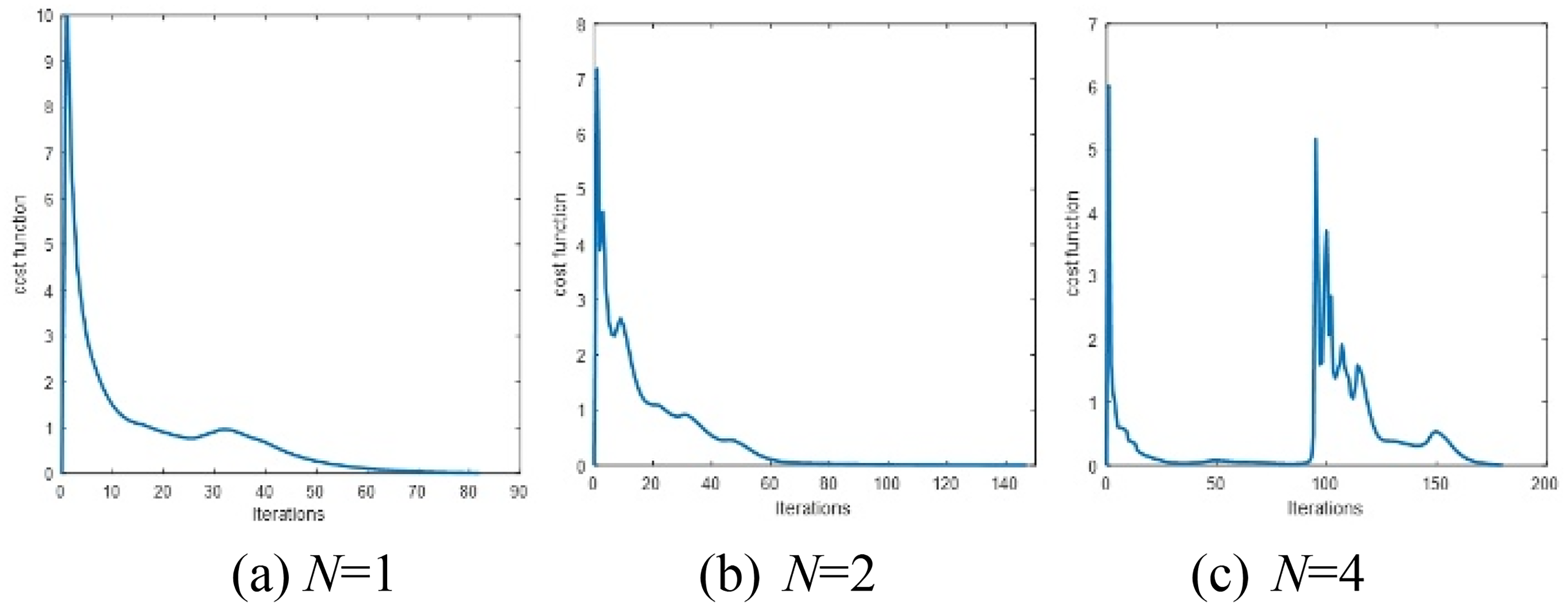
Cost function values for different numbers of obstacles. (a) N = 1. (b) N = 2. (c) N = 4.
Different numbers of obstacles.

The size, number, and distribution of the obstacles and the number of robots were varied in the above four simulations. In the non-convex area, the CVT algorithm has a good control effect on the swarm robotics, and its efficiency is not affected by the size of the obstacles. The position of the objects has little effect on the formation, and its efficiency is affected only by the number of robots. Thus, the constrained CVT algorithm can realize the formation control of swarm robotics.
Optimal Number of Robots
This section verifies how to determine the optimal number of robots given the size of the task area. If the number of robots is too small, it is difficult to achieve full coverage of the task area. Conversely, if the number of robots is too large, it will lead to resource wastage. Therefore, it is necessary to determine the optimal number of robots to achieve coverage of the entire target area.
Determining the initial number of robots
Firstly, consider the basic perception model of the robots, as illustrated in Figure 15. Here,
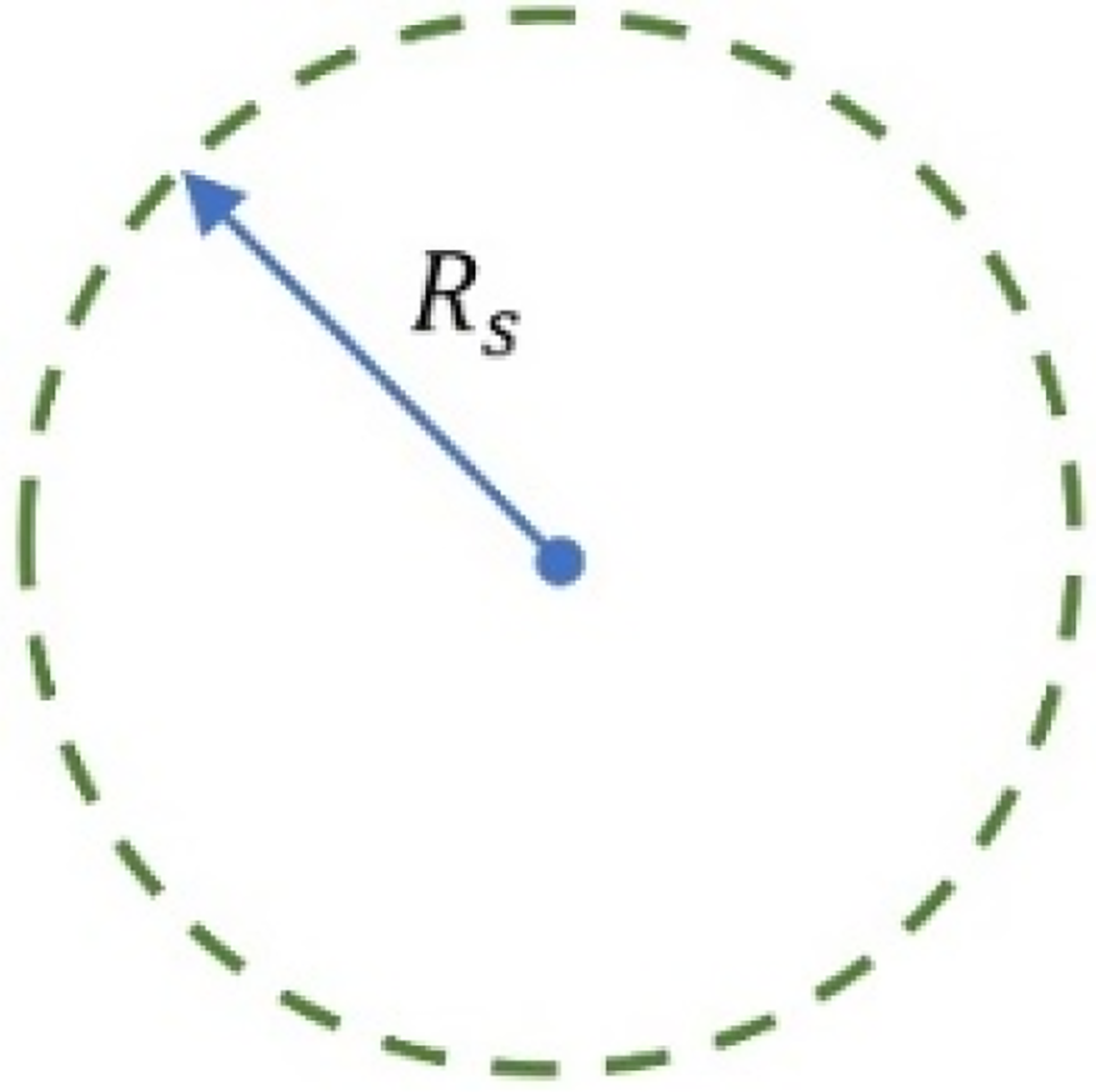
Perception mode.
Therefore, for any robot node 

Area coverage.
The communication diameter of a robot is defined as


Determining the optimal number of robots
Typically, the methods mentioned in the previous section are only used to determine the initial number of robots, while the specific optimal number of robots needs to be determined based on different task requirements and performance metrics. Two common coverage performance evaluation metrics are defined as follows:
Coverage rate Coverage efficiency
The node coverage rate is used to evaluate the extent to which robots cover the task area. It is determined by the ratio of the sum of the coverage areas of robot nodes to the total area of the task area, calculated as:
Robot node coverage efficiency is mainly used to measure the utilization rate of robot node coverage. A higher value indicates a higher utilization rate of robot node coverage. It is determined by the ratio of the sum of effective coverage areas of robot nodes to the sum of all robot perception range areas, calculated as:
Experimental parameter settings.
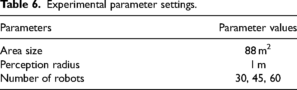
In this experiment, the quantities of robots selected are 30, 45, and 60 respectively, with the obstacle's central position set at (5,5). The experimental results are illustrated in Figure 17. Figure 18 presents the variations in the cost function for different numbers of robots. The cost function reaches its minimum values at iterations 128, 228, and 231 respectively. Experimental data are detailed in Table 7.

CVT for different numbers of robots. (a) n = 128. (b) n = 228. (c) n = 231.

Cost function value for different numbers of robots
Performance metrics under different numbers of robots.

According to Table 7 and Figure 17, it can be observed that as the number of robots continues to increase, the overall coverage efficiency decreases continuously.
However, based on the principle of robot coverage efficiency formula, it is understood that with a constant task area, a smaller number of robots ensures a smaller overlapped coverage area, resulting in higher node coverage efficiency. As the number of robots increases, the overlapped area grows, leading to a decrease in node coverage efficiency while the coverage rate of robots increases. Therefore, the selection of the optimal number of robots needs to be dynamically adjusted based on the requirements of the task. Starting from the initial number of robots obtained, a higher coverage rate requires an increase in the number of robots, while a higher coverage efficiency necessitates a reduction in the number of robots.
Swarm robotics experiment
ROS robot formation control
The experiments conducted in this study used the Turtlebot3 robot, which is a low cost, development friendly mobile robot platform based on the robot operating system (ROS). Each Turtlebot3 can independently build a local map of its surroundings through the mapping function package of ROS, which provides SLAM (simultaneous localization and mapping) for LiDAR and a grid-based 2D map based on the LiDAR input and attitude data. In the actual experiment, the robot's motion model is a second-order dynamics model. The lab map was selected as the designated area for the robot formation Q. The area was free of obstacles, as shown in Figure 19(a). Four Turtlebot3 robots were randomly placed on the map, and the robots used the SLAM technology to complete their positioning. The results of the experiment are shown in Figure 19(b). The experiments were set such that when the Voronoi cost function reached the optimal solution, the robots reached the position required for the desired formation under that density function, that is, they achieved the target formation. The difference between the simulation and actual experiment was that the density function was not initialized as a constant at the initial stage of the experiment, but rather, the target expected formation was determined before the commencement of the experiment.

Experimental environment for multi-robot formation. (a) Experimental. (b) SLAM map (RVIZ).
When the density function was set to a constant, the map was evenly divided into four generated points, as shown in Figure 20(a). Figure 20(c) shows the initial position of the robot. The CVT algorithm converged when the number of iterations was approximately 200, as shown in Figure 20(b), at which point the cost function reached its minimum value. The robots completed a square formation on the map, as shown in Figure 20(d).
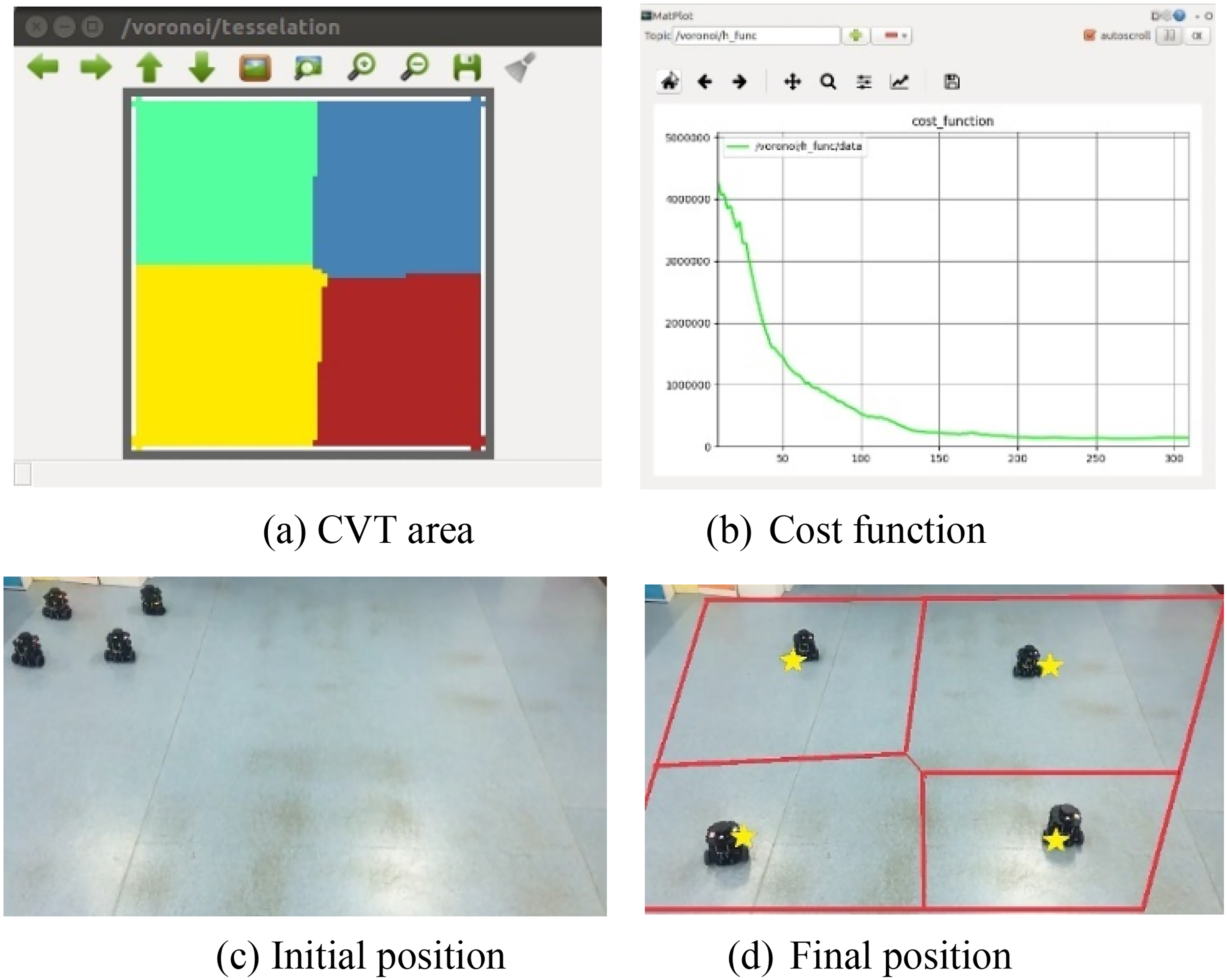
Square formation experiment. (a) CVT area. (b) Cost function. (c) Initial position. (d) Final position.
Figure 21(a) depicts the Voronoi partition under the “V”-shaped density function. The initial positions of therobots are shown in Figure 21(c). Figure 21(b) depicts the cost function for the “V”-shaped distribution of the density function. The initial value of the cost function was approximately 6.3 × 10⁴. When the CVT algorithm converged after approximately 120 iterations, the robots completed a straight formation, as shown in Figure 21(d).

Line formation experiment. (a) CVT area. (b) Cost function. (c) Initial position. (d) Final position.
The algorithm was also validated on the dynamic formations achieved with four Turtlebot3 robots. The experiments involved dynamic formations in the obstacle-free and random obstacle scenarios. The robots were initially positioned in the upper left corner of the map, marked by stars in Figure 22(a) and (b). The target point was located in the lower right corner of the map, marked by red flags in Figure 22(a) and (b), and the black line denotes the motion trajectory of the multi-robot system. We modified the map created by SLAM. The obstacles of irregular shapes in the original map were transformed into circular obstacles, as shown in Figure 22 (c). The modified map was used as the environmental information for the robots.

SLAM map. (a) Obstacle-free. (b) Random obstacles. (c) Circular obstacles.
Obstacle-free scene (convex)
As shown in Figure 23, the experimental scene can be regarded as a rectangle and there were no obstacles in the area, which represented a convex environment. The robots were in the upper left of the area at the instant t1. The Voronoi tessellation algorithm converged when the robots reached the centroid of each Voronoi cell, as shown is Figure 23(a). Figure 23(b) and (a) shows that the robots move to the target point at the instants t3 and t4, respectively. Finally, they reach the target at t4 as shown in Figure 23(d). In comparison with the traditional CVT, our improved CVT can divide the area in a non-convex environment as well, which allows the robots to move to the target point in a suitable formation.

Convex (obstacle-free) scene. (a) t1 = 0 s. (b) t2 = 64 s. (c) t3 = 75 s. (d) t4 = 120 s.
Randomly distributed obstacles scene (non-convex)
To verify the feasibility of the constrained CVT, we added obstacles to the scenario shown in Figure 23 to transform it to a non-convex environment, as shown in Figure 24 The robots were positioned in the upper left of the map at the instance t1. In Figure 24(a), all robots reached the centroid of each Voronoi cell. Then, the constrained area Q moved along the desired direction while obtaining the two- dimensional map information as the region density. For a non-zero threshold, we set the density value to zero so that the robots could avoid the obstacles, as shown in Figure 24(b) and (c). In Figure 24(d), the robots reached the desired position at t4. The experiment showed that the constrained CVT could separate the non-convex environment from the obstacles to ensure that the robots could bypass the obstacles and reach the target position. This proved the feasibility of the algorithm for a non-convex environment.
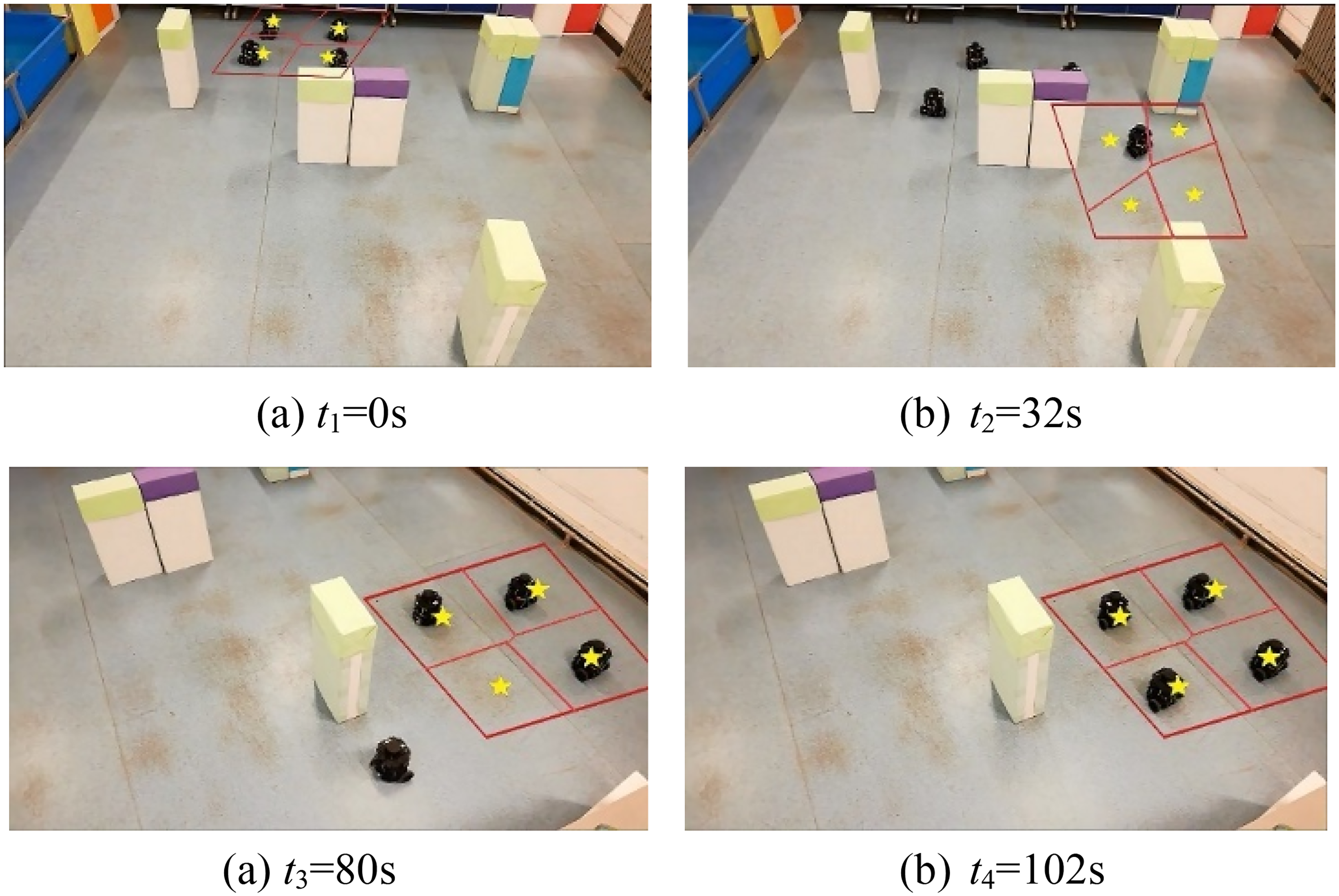
Random obstacles. (a) t1 = 0 s. (b) t2 = 32 s. (c) t3 = 80 s. (d) t4 = 102 s.
In summary, the experimental results showed that the constrained CVT algorithm could be applied to both convex and non-convex regions. The time consumed by the algorithm was 120 s for the experiment on the convex area and 102 s for the experiment on the non-convex area. The results are consistent with the simulation results in Section 4.2-A. It can be inferred from the experiments that for regions of the same size, obstacles in the non-convex region reduce the area that can be effectively divided as well as the number of iterations; hence, the process is less time consuming when compared with the convex region.
Conclusion and future work
This study successfully applied the CVT algorithm to the ROS, saving a lot of research work. Through the CVT algorithm, the central processing unit processes position information and sends particle information from the CVT partition to each robot as its target point, thereby achieving control over multiple robots. Compared to other multi-robot system designs, the CVT algorithm converges to the centroid of each Voronoi cell, and each robot moves within its Voronoi cell, which can minimize collisions. The performance of the algorithm was validated through 5 different simulations, and the results showed that the constrained CVT algorithm is not sensitive to the size and position of obstacles, but an increase in the number of robots will increase the total number of iterations. The optimal number of robots needs to be dynamically selected based on different performance indicators. The experimental results show that using the CVT algorithm can ensure that multiple robots form a formation according to the optimal distribution in the designated area, while increasing the redundancy and robustness of the system. Easy to dynamically switch formations based on external environment, improving the flexibility and scalability of formations. However, the current method assumes that all robots are in good condition and have the same power consumption, and future research will consider more practical scenarios, such as irregular and dynamic obstacle environments.
Footnotes
Acknowledgements
This study was co-supported by the funds of National Natural Science Foundation of China Youth Fund (62103315, 62303368); Key R & D Projects in Shaanxi Province (2022GY-238); Special Project for Guiding Technological Innovation in Shaanxi Province (2022QFY01-16, 2023-ZDLNY-61); Ministry of Education Key Laboratory of Information Fusion Technology Open Fund Project (Project No. 202312-IFTKFKT-007).
Declaration of conflicting interests
The authors declared no potential conflicts of interest with respect to the research, authorship, and/or publication of this article.
Funding
The authors disclosed receipt of the following financial support for the research, authorship, and/or publication of this article: This work was supported by the Key R & D Projects in Shaanxi Province, Ministry of Education Key Laboratory of Information Fusion Technology Open Fund Project, National Natural Science Foundation of China Youth Fund, Special Project for Guiding Technological Innovation in Shaanxi Province (grant numbers 2022GY-238, 202312-IFTKFKT-007, 62103315, 62303368, 2022QFY01-16, 2023-ZDLNY-61).