Sage Journals: Discover world-class research

Abstract

This article presents a novel learning-based optimal control approach for dynamic control of continuum robots. Working and interacting with a confined and unstructured environment, nonlinear coupling, and dynamic uncertainty are only some of the difficulties that make developing and implementing a continuum robot controller challenging. Due to the complexity of the control design process, a number of researchers have used simplified kinematics in the controller design. The nonlinear optimal control technique presented here is based on the state-dependent Riccati equation and developed with consideration of the dynamics of the continuum robot. To address the high computational demand of the state-dependent Riccati equation controller, the distilled neural technique is adopted to facilitate the real-time controller implementation. The efficiency of the control scheme with different neural networks is demonstrated using simulation results.

Keywords

Deep learning neural networks knowledge distillation SDRE control continuum robot control

Introduction

Continuum robotics has made considerable strides in recent years and currently encompasses a diverse variety of applications and technologies. In contrast to most traditional robots comprising rigid linkages, continuum robots (CRs) have flexible parts that enable them to deform continuously, making them ideal for applications requiring intricate motions, ranging from industrial maintenance to surgical operations and space deployment systems.^1

–7

CRs provide a number of benefits over rigid robots, that is, they can operate in restricted and congested environments and manipulate a variety of shapes and types of objects owing to their flexibility without excessive mechanical parts complexity.

Despite the benefits of CRs discussed above, modeling and control of CRs present difficult challenges due to the high level of dynamic complexity, coupling, and nonlinearity. In general, the deformation of CRs may be represented by a suitable kinematics model, which is also a focus of study in the literature; however, such models do not give insight into dynamic behavior. Furthermore, the high-speed movements and inertia decrease the robot’s kinematic model accuracy significantly. Therefore, for accurate control it is necessary to explore the CR dynamic model to analyze the relationship between driving force and bending deformation.⁸

In the literature, four approaches for dynamic modeling of CRs have been presented, including Lagrangian method,⁹ Cosserat rod theory,¹⁰ constant deformation,¹¹ and center of gravity.¹² The Lagrangian technique is used for dynamic modeling of the CR in this work, because of its computational efficiency and ease of real-time implementation.¹³ However, the Lagrangian approach described in He et al.⁹ lacked a general formulation and relied predominantly on Taylor series expansion and several curve fittings to simplify the CR equations. For these reasons, an appropriate technique (adapted from Samadikhoshkho et al.¹³) is required to handle CR modeling issues in the initial stage of designing the controller.

An effective dynamic control strategy is also required to deal with the system’s complicated behavior. Numerous prior publications have concentrated on the kinematic control of cable-driven CRs,¹⁴ with only a few addressing their dynamic control.^15
–17 The inherent difficulty in designing a controller for a dynamic model is the primary reason that a limited number of works exist on dynamically controlled CRs. More studies have been conducted on the dynamic modeling and control of pneumatically actuated robots^18
–20 than on cable-driven robots.^21
–23

Along with model-based control strategies for CRs, there are model-free control methods that utilize machine learning.²⁴ Machine learning research to control CRs often employs a supervised learning technique^25

–29 or reinforcement learning (RL).^30,31 Supervised learning approaches are predicated on having the correct answer to the issue available and attempting to learn from it. In Giorelli et al.,²⁵ a feed-forward neural network was trained to learn the inverse kinematics of a cable-driven CR. An experimental study with the same approach²⁵ was again conducted by Giorelli et al.²⁶ In Xu et al.,²⁸ the inverse kinematics of the robot was determined using three regression methods, including extreme learning machine, Gaussian mixture regression, and k-nearest neighbors regression. In Bern et al.,²⁹ a neural network was trained to learn the forward kinematics of a soft robot; and an optimal open-loop controller was designed using a gradient-based optimization method.

In RL, a learning agent is rewarded after each action; and this reward indicates how beneficial the activity was. The objective of RL is to discover an optimal policy that maximizes the agent’s cumulative reward over the course of an episode. A reinforcement approach based on a Q-learning algorithm was employed in You et al.³⁰ to control a soft manipulator in a 2D plane. In Liu et al.,³¹ proximal policy optimization algorithm was used for locomotion control of a soft snake robot.

RL has several drawbacks. For example, solving a problem with RL requires an appropriate reward function, which can be very challenging to formulate. In addition, every RL algorithm has several hyper-parameters, such as discount factor and time horizon, that significantly affect the solution and need to be carefully tuned. In the present work, a supervised approach is developed based on a specific type of nonlinear optimal control scheme, the state-dependent Riccati equation (SDRE) technique,³² to optimally control a CR’s dynamics. An optimal control strategy should leverage the flexibility of CRs to advance present applications and incorporate online application in congested, dynamic, and unstructured environments.³³

Although SDRE is a powerful control method that is a nonlinear generalization of the linear quadratic regulator controller, it has rarely been used in the past due to its high computational cost, particularly prior to the development of fast computers and learning approaches in recent years. For example, neural SDRE control of the dynamics of a satellite’s attitude³⁴ is a recently developed solution for real-time application of the SDRE method. The dynamics of a CR are more complex than those of a satellite, making SDRE control design and implementation for CRs more challenging. To the best of the authors’ knowledge, no optimal SDRE control strategy has yet been developed for CRs due to the complexity of their dynamics.

The purpose of this article is to introduce a novel end-to-end learning-based strategy for dynamic control of a cable-driven CR. Following the training of neural networks to replicate the SDRE controller, the knowledge distillation (KD) method³⁵ is used to train smaller networks on the basis of previously trained larger ones. Although KD has been mostly applied to classification issues, here it is modified for the regulation challenge. KD enables training smaller networks with fewer parameters while leveraging prior knowledge from larger networks. Additionally, it has a regularization impact that may help networks achieve greater generality. The impact of several network designs is investigated to determine the best effective architecture and learning technique for neural SDRE control of CRs.

Dynamic modeling

Dynamic modeling of a tendon-driven CR, shown in Figure 1, is provided in this section by adapting from Samadikhoshkho et al.¹³ and focusing exclusively on the CR described in that work.

Figure 1.

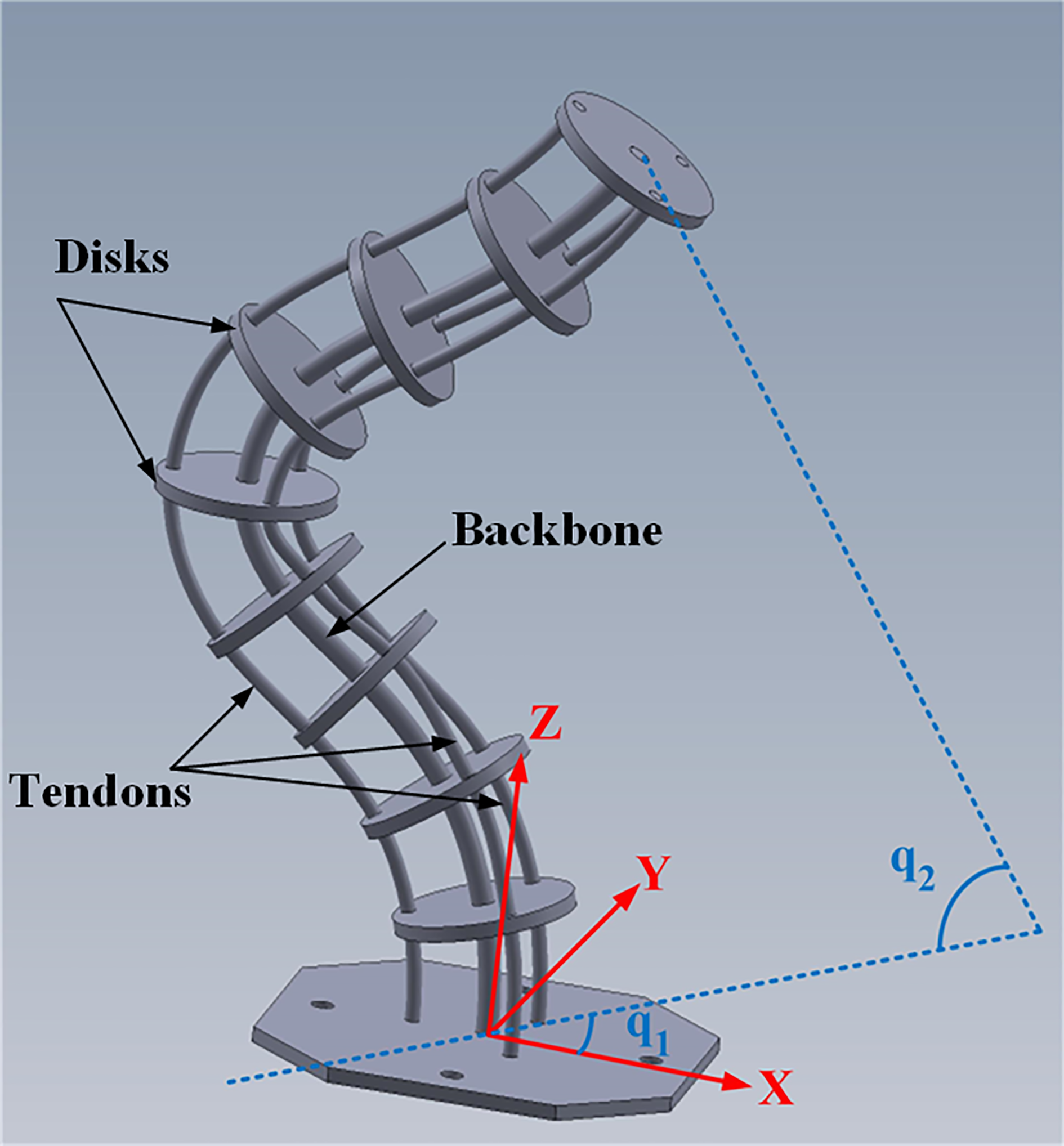
Continuum robot rendering of components and end-effector angles.

Controllable degrees of freedom for a tendon-driven CR are denoted by vector $q$ in equation (1), including two angles q ₁ and q ₂

q = {[\begin{matrix} q_{1} & q_{2} \end{matrix}]}^{T}

where q ₁ is the horizontal angle of the end-effector with respect to X-axis in the XY plane, and q ₂ is the vertical angle of the end-effector with respect to the Z-axis.

To model a flexible continuum arm, it is first necessary to consider a section of the CR and find its kinematics and energy functions. Then, by taking the integral along the length of the CR, the dynamics of the CR can be derived using Euler–Lagrange theory. The position of the end-effector can be determined by rotating the flexible arm coordinate (given by the flexible beam model⁹) about the Z-axis by the angle q ₁. In addition, the end-effector orientation (rotation matrix) can be found by performing three rotations around the Z-axis for angle q ₁, the Y-axis for angle q ₂, and the Z-axis for angle $- q_{1}$ , respectively.⁹

The rotation matrix between a point of arm at section s and the base of the arm $R_{s}$ can be found in Godage et al.³⁶ and expressed as equation (2)

R_{s} = [\begin{matrix} n_{s} & b_{s} & t_{s} \end{matrix}]

where vectors $n_{s}$ , $b_{s}$ , and $t_{s}$ are columns of the rotation matrix.

The angular velocity of each section of arm $ω_{s}$ is obtained as³⁷

ω_{s} = skew (t_{s}) {\dot{t}}_{s} = J_{o} (s) \dot{q}

where $skew ()$ denotes the skew-symmetric form and $J_{o} (s)$ is the orientation Jacobian matrix at section s. The linear velocity of arm at section s is also determined as

{\dot{p}}_{s} = J_{p} (s) \dot{q}

where $J_{p} (s)$ represents the position Jacobian matrix at section s.

By considering Euler–Lagrange formulation, equation (5), a dynamic model of the robot can be derived. To define the Lagrangian of the system, $ℒ$ , calculating system’s kinetic energy $K$ and potential energy $U$ are required

ℒ = K - U

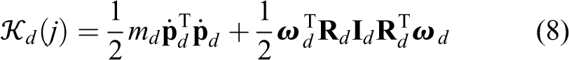
The kinetic energy of the robot consists of two parts. The first part is related to the main backbone denoted by $K_{m . b}$ , and the second part is the total kinetic energy of disks, $K_{d}$ . Energy in energy is neglected as it has a negligible effect on the system dynamics

K = K_{m . b} + K_{d}

Kinetic energy of the backbone at each section s, $K_{m . b} (s)$ is obtained from equation (7)

K_{m . b} (s) = \frac{1}{2} ρ_{s} A_{s} {\dot{p}}_{s}^{T} {\dot{p}}_{s} + \frac{1}{2} ω_{s}^{T} R_{s} I_{s} R_{s}^{T} ω_{s}

where $ρ_{s}$ , A_s , and $I_{s}$ are the backbone’s density, cross section, and moment of inertia matrix, respectively. Similarly, the kinetic energy of the j-th disk $K_{d} (j)$ is calculated as

K_{d} (j) = \frac{1}{2} m_{d} {\dot{p}}_{d}^{T} {\dot{p}}_{d} + \frac{1}{2} ω_{d}^{T} R_{d} I_{d} R_{d}^{T} ω_{d}

where

p_{d} = {p_{s} |}_{s = j h}, j = 1, 2, ..., n

ω_{d} = {ω_{s} |}_{s = j h}, j = 1, 2, ..., n

R_{d} = {R_{s} |}_{s = j h}, j = 1, 2, ..., n

in which h, n, m_d , and $I_{d}$ denote distance between disks, number of disks, mass and moment of inertia of each disk, respectively. Finally, the total kinetic energy of the robot, $K$ , is expressed as

K = \int_{s = 0}^{l} K_{m . b} (s) d s + \sum_{j = 1}^{n} K_{d} (j)

where l is the length of the backbone.

By using equations (3) and (4), the total kinetic energy can be written as

K = \frac{1}{2} {\dot{q}}^{T} M \dot{q}

where

\begin{array}{l} M = \int_{s = 0}^{l} (ρ_{s} A_{s} J_{p}^{T} (s) J_{p} (s) + J_{o}^{T} (s) R_{s} I_{s} R_{s}^{T} J_{o} (s)) d s \\ + \sum_{j = 1}^{n} {(m_{d} (j) J_{p}^{T} (s) J_{p} (s) + J_{o}^{T} (s) R_{d} I_{d} R_{d}^{T} J_{o} (s)) |}_{s = j h} \end{array}

Similarly, the potential energy of the robot $U$ consists of two parts, $U_{m . b}$ and $U_{d}$ , which are presented in equations (13) to (15) as follows

U = U_{m . b} + U_{d}

U_{m . b} = \int_{s = 0}^{l} (ρ_{s} A_{s} g e_{3}^{T} p_{s}) d s + \frac{2 E_{s} I_{s}}{l} q_{2}^{2}

U_{d} = \sum_{j = 1}^{n} {(m_{d} (j) g e_{3}^{T} p_{s}) |}_{s = j h}

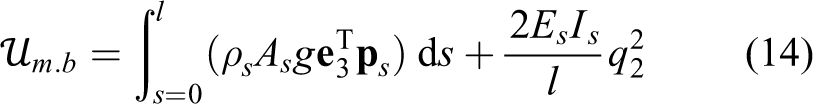
where g is the acceleration due to gravity, e ₃ shows direction of gravity, and E_s denotes Young’s modulus of the main backbone. Potential energy storage in cables is neglected.

Finally, using equations (11) and (13) to (15), the dynamic model of the system is derived as equation (16)

M (q) \ddot{q} + C (q, \dot{q}) \dot{q} + G (q) = u

where

\begin{array}{l} C_{i j} = \frac{1}{2} \sum_{k = 1}^{2} (\frac{\partial M_{i j}}{\partial q_{k}} + \frac{\partial M_{i k}}{\partial q_{j}} - \frac{\partial M_{k j}}{\partial q_{i}}) {\dot{q}}_{k} \end{array}

G (q) = {(\frac{\partial U (q)}{\partial q})}^{T}

Although the CR has an infinite number of degrees of freedom, only two angles of the end-effector can be controlled by the robot actuators pulling tendons. Therefore, the end-effector position can be changed by adjusting the end-effector angles. Three tendons are responsible for controlling the tendon-driven CR under consideration. The first tendon actuator is positioned along the X-axis, while the other two are each placed at an angle of 120° with respect to the first tendon. Based on the horizontal angle of the end-effector, two tendons should function. Tendons 1 and 2 should be activated if q ₁ is between 0° and 120°. Similarly, tendons 2 and 3 should be involved for $120 < q_{1} < 240$ , whereas tendons 1 and 3 are responsible for $240 < q_{1} < 360$ .

The relation between the control signal and tendons tensions $F_{ten} = [F_{1} F_{2} F_{3}]^{T}$ is expressed as equation (19) (as stated in Samadikhoshkho et al.¹³)

u = D_{ten} F_{ten}

where $D_{ten}$ is calculated based on tendon displacement in Samadikhoshkho et al.¹³

Control design

This section discusses the development of the model-based optimal control and learning approach for controlling a CR.

State-dependent Riccati equation

The presented model of the CR in the preceding section reveals a high degree of nonlinearity in the system dynamics. Therefore, linear control techniques may be inapplicable to such a nonlinear system. To deal with the nonlinearity issue and to improve the robustness of the controller, the SDRE approach is suggested to compute the control’s optimal solution at each time step.

To design the controller, it is necessary to first describe the nonlinear equations in a pseudo-linear form with state-dependent coefficients. It is common to express the pseudo-linear structure in the form shown in equation (20); however, a new representation is required to adapt the equations for CR dynamics, as seen in equation (21)

\dot{x} = A (x) x + B (x) u

\dot{x} = A (x) x + B (x) u + F (x)

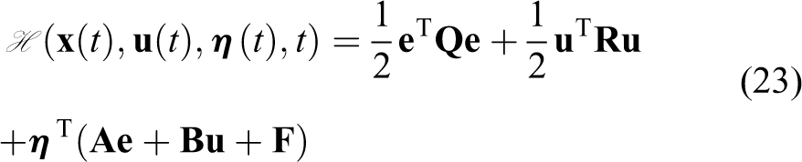
For optimal reference tracking problem of the system presented in equation (21), the error vector is defined as $e = x - x_{d}$ , where $x_{d}$ denotes the desired state vector (reference).

The control problem is to find the optimal solution for the system by minimizing the following performance measure (cost function), J

J = \frac{1}{2} \int_{0}^{\infty} (e^{T} Q e + u^{T} R u) d t

where $Q$ and $R$ are positive definite weight matrices for tracking and control effort costs, respectively. To calculate the optimal control signal, the Hamiltonian $ℋ (x (t), u (t), η (t), t)$ is written as equation (23) as cited in Kirk.³⁸ Here, $η$ depicts co-states

\begin{matrix} ℋ (x (t), u (t), η (t), t) = \frac{1}{2} e^{T} Q e + \frac{1}{2} u^{T} R u \\ + η^{T} (A e + B u + F) \end{matrix}

The optimal control gain can be derived by finding the solution for equation (24) (as stated in Kirk³⁸).

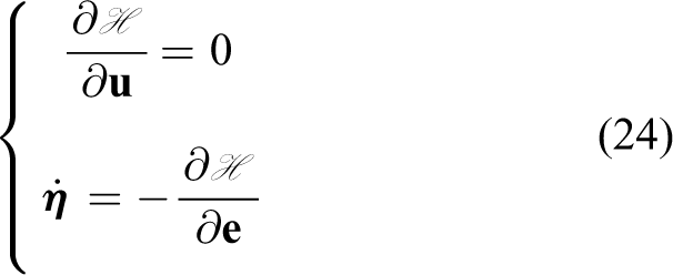
{\begin{matrix} \frac{\partial ℋ}{\partial u} = 0 \\ \dot{η} = - \frac{\partial ℋ}{\partial e} \end{matrix}

which results in

R u + B^{T} η = 0

25a

- Q e - A^{T} η = \dot{η}

25b

By defining $η = P e - g$ and substituting in equation (25a), one can obtain

u^{*} = - R^{- 1} B^{T} (P e - g) = K_{1} e + K_{2}

where $P$ and $g$ terms are defined later, $K_{1} = - R^{- 1} B^{T} P$ and $K_{2} = R^{- 1} B^{T} g$ . Substituting the optimum control signal equation (26) into equation (25b) and using the error dynamics, $\dot{e} = A e + B u + F$ , the following expression emerges

\begin{matrix} - Q e - A^{T} (P e - g) = \dot{η} = \dot{P} e + P \dot{e} + \dot{g} \\ = \dot{P} e + P [A e + B (- R^{- 1} B^{T}) (P e - g) + F] \end{matrix}

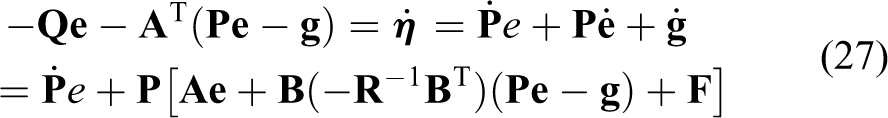
which can be rearranged as

\begin{array}{l} (\dot{P} + P A + A^{T} P + Q - P B R^{- 1} B^{T} P) e \\ + (P B R^{- 1} B^{T}) g + P F = 0 \end{array}

The solution of equation (28) leads to the following equations

\dot{P} + P A + A^{T} P + Q - P B R^{- 1} B^{T} P = 0

29a

(P B R^{- 1} B^{T}) g + P F = 0

29b

The expression in equation (29a) is a well-known Riccati equation, which can be solved for steady-state conditions (to facilitate its real-time application) as seen in equation (30) by setting $\dot{P} = 0$ .

P A + A^{T} P + Q - P B R^{- 1} B^{T} P = 0

By solving the Riccati equation and finding $P$ , $g$ is calculated by substituting $P$ into equation (29b) as

g = (A^{T} - P B R^{- 1} B^{T})^{- 1} P F

Finally, having $P$ and $g$ , the optimum control signal can be found from equation (26). For the CR problem, the state variables are selected as

x = {[\begin{matrix} q_{1} & q_{2} & {\dot{q}}_{1} & {\dot{q}}_{2} \end{matrix}]}^{T}

Also, the quadratic form of the CR equation, equation (16), can be rewritten by expressing equation (21) as

\dot{x} = [\begin{matrix} 0_{2 \times 2} & I_{2 \times 2} \\ 0_{2 \times 2} & - M^{- 1} C \end{matrix}] x + [\begin{matrix} 0_{2 \times 2} \\ M \end{matrix}] u + [\begin{matrix} 0_{2 \times 1} \\ - M^{- 1} G \end{matrix}]

Data acquisition and learning procedure

This work employs a supervised approach to solve the reference tracking problem. Supervised learning aims to estimate the mapping between given input–output pairs, which can then be used to predict the output for any new input. In the scenario under consideration for CR control, the mapping to be estimated is an SDRE controller that receives the dynamical system’s state variables and desired states as inputs and produces the appropriate control signals as outputs.

The training data are generated by the SDRE control technique presented in the previous section. Since there is a reference tracking problem for CR control, both state vector $x$ and error vector $e = x - x_{d}$ are used to find the optimal control signal. Hence, the input of each training sample is defined as

x_{e} = [\begin{matrix} x \\ e \end{matrix}]

To train the network, inputs are randomly generated within the appropriate range, and the corresponding outputs are calculated by the SDRE controller. The output of each sample has two potential alternatives, both of which are tried. The first option is to predict the SDRE control gains, $K_{1}$ and $K_{2}$ , and calculate control signal using $u^{*} = K_{1} e + K_{2}$ . The second, and more straightforward, alternative is to use control signal $u$ as the output signal, which may result in predicting fewer values because $u$ has the same dimension as $K_{2}$ .

Several types of neural networks can be used to address regression issues, and the problem setup should determine the most appropriate one. The input to the SDRE controller for the CR is a vector with no spatial link between its members, that is, the order of the vector elements is chosen arbitrarily before deriving the dynamical system governing equations of motion. Additionally, because there are no temporal trends in the data, all samples are independent and identically distributed. This is because the SDRE controller computes the control signal only based on the system’s present state and disregards past states. The present work uses multilayer perceptron (MLP) neural networks.

A schematic structure of a simple MLP artificial neural network with input size n, output size c, and two hidden layers is shown in Figure 2. In each neuron (shown as circles in Figure 2), input $x$ is multiplied by the weight vector of the neuron $W$ and a bias b is added. Finally, an activation function $σ (.)$ is applied to generate the output of the neuron. Therefore, the output of j-th neuron in the i-th layer can be calculated using equation (35)

y_{j}^{(i)} = σ (W_{j}^{(i)}^{T} x^{(i)} + b_{j}^{(i)})

where the input of layer $(i)$ , $x^{(i)}$ , is the output of layer $(i - 1)$ . Network parameters must be determined by minimizing an appropriate loss function between network outputs (predictions) and desired outputs.

Figure 2.

A multi-layer perceptron neural network—input, layers, and output.

Following training, the neural network is expected to perform well not only on the training data but also on previously unseen test data. This is referred to as generalization, and it is one of the most challenging aspects of machine learning. Another critical issue in particular applications, such as control of CRs, is the size of the neural network (number of parameters). Reducing size of the network can increase its generalization and speed up its execution; however, simply decreasing the size is frequently not a wise approach, because it reduces the network’s complexity and capability to learn increasingly more complicated tasks.

KD³⁵ is a technique for training smaller networks based on what a larger network has already learned, similar to the concept of fitting data to functions or reducing the order of a set of governing differential equations. Initially, KD was presented as a solution to the classification problem. According to KD, when a large network is trained to solve a classification task, the layer preceding the softmax provides an appropriate embedding for the input data. Hinton et al.³⁵ recommended concurrently training a smaller network that predicts this embedding and labels the sample. This approach is adopted for CR control in this article.

KD begins with training of a large neural network (teacher network) to solve the regression issue by minimizing the mean squared error (MSE) between network outputs and desired outputs. As indicated in Figure 3, a smaller network (student/distilled network) is then trained in such a way that its output layer accurately predicts the desired outputs, while one of its hidden layers predicts the embedding, $z^{teacher}$ , generated by one of the teacher network’s hidden layers. The loss function for training the student network can be defined as sum of two MSE loss functions presented in equation (36)

Loss = α L_{student} + (1 - α) L_{distillation}

where

L_{student} = MSE (y^{student}, y^{desired})

L_{distillation} = MSE (z^{student}, z^{teacher})

Figure 3.

The proposed knowledge distillation structure.

Notably, the teacher is not trained during the student network’s training, and back-propagation is performed only on the student network.

In a regression problem with c outputs, there are two types of neural network architectures based on their outputs. The architecture can be either a single network with c outputs or a set of c separate networks with a single output. For KD, if the teacher network is trained with the second scenario (separate networks for outputs), then they can either be distilled separately or the foremost can be merged and then distillation is performed. The performance of these different scenarios will be compared in simulation results section.

The Block diagram of the closed-loop system is shown in Figure 4, in which Controller and System refer to the trained neural network and the dynamic model of the system presented by equation (33), respectively.

Figure 4.

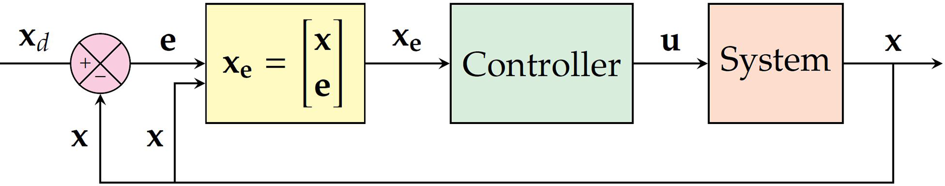
The suggested Block diagram for the closed-loop control of CRs. CR: continuum robot.

Simulation results

Simulation was used to assess the efficiency of the proposed neural-based SDRE control approach for tendon-driven CRs with the exact specification as Samadikhoshkho et al.¹³ Several networks were trained and compared to determine the best neural controller structure for this CR.

The input dimension of all networks is eight, including four states and four error variables. Different neural network cases are considered as follows:

a single network with output of the control signal $u = [u_{1}, u_{2}]^{T}$ ;

two networks with output of u ₁ and u ₂;

two teacher networks with outputs of u ₁ and u ₂ trained separately, then merged and distilled to a single student network with the output of $\hat{u} = [{\hat{u}}_{1}, {\hat{u}}_{2}]^{T}$ ; and

two teacher networks with outputs of u ₁ and u ₂ trained and distilled separately to networks with outputs of ${\hat{u}}_{1}$ and ${\hat{u}}_{2}$ , then merged.

In case (1), the network has three intermediate (hidden) layers with 500, 500, and 100 neurons while the output layer has two neurons. In case (2), both u ₁ and u ₂ networks have three intermediate layers and an output layer with 200, 100, 50, and 1 neuron, respectively. In both cases, intermediate layers have “PReLu” activation function.

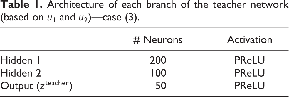
In case (3), for both u ₁ and u ₂ networks, networks from case (2) after eliminating their last layers are used. This architecture is shown in Table 1. To form the teacher, networks u ₁ and u ₂ are concatenated so that the output has two components. This teacher network is then distilled into the student network with the architecture shown in Table 2.

Table 1.

Architecture of each branch of the teacher network (based on u ₁ and u ₂)—case (3).

	# Neurons	Activation
Hidden 1	200	PReLU
Hidden 2	100	PReLU
Output ( $z^{teacher}$ )	50	PReLU

Table 2.

Architecture of distilled network—case (3).

	# Neurons	Activation
Hidden 1	25	PReLU
Hidden 2	25	PReLU
Hidden 3 ( $z^{student}$ )	50	—
Hidden 4	25	PReLU
Hidden 5	25	PReLU
Output	2	—

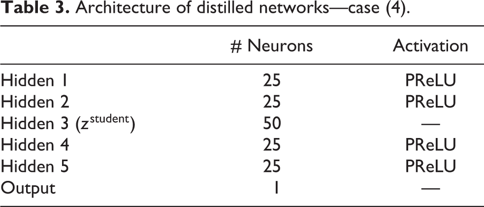
In case (4), each teacher network is identical to that of case (3); however, they are separately distilled to networks with architectures presented in Table 3. Then, these separately distilled networks are augmented and used as controller. Each distilled network has 4130 trainable parameters, which is significantly less than the teacher network with 26,953 parameters.

Table 3.

Architecture of distilled networks—case (4).

	# Neurons	Activation
Hidden 1	25	PReLU
Hidden 2	25	PReLU
Hidden 3 ( $z^{student}$ )	50	—
Hidden 4	25	PReLU
Hidden 5	25	PReLU
Output	1	—

Distillation loss in equation (38) is defined as MSE between the output of the third hidden layer of the u-network and the third hidden layer of the distilled network, both of which have a dimension of 50. The student loss is defined as MSE between the output of the distilled network and the ground truth.

To evaluate the performance of the proposed neural network controllers, the following desired trajectory for a circular motion of the end-effector is considered

x_{d} (t) = {[\begin{matrix} \frac{π}{8} t & \frac{π}{9} & \frac{π}{8} & 0 \end{matrix}]}^{T}

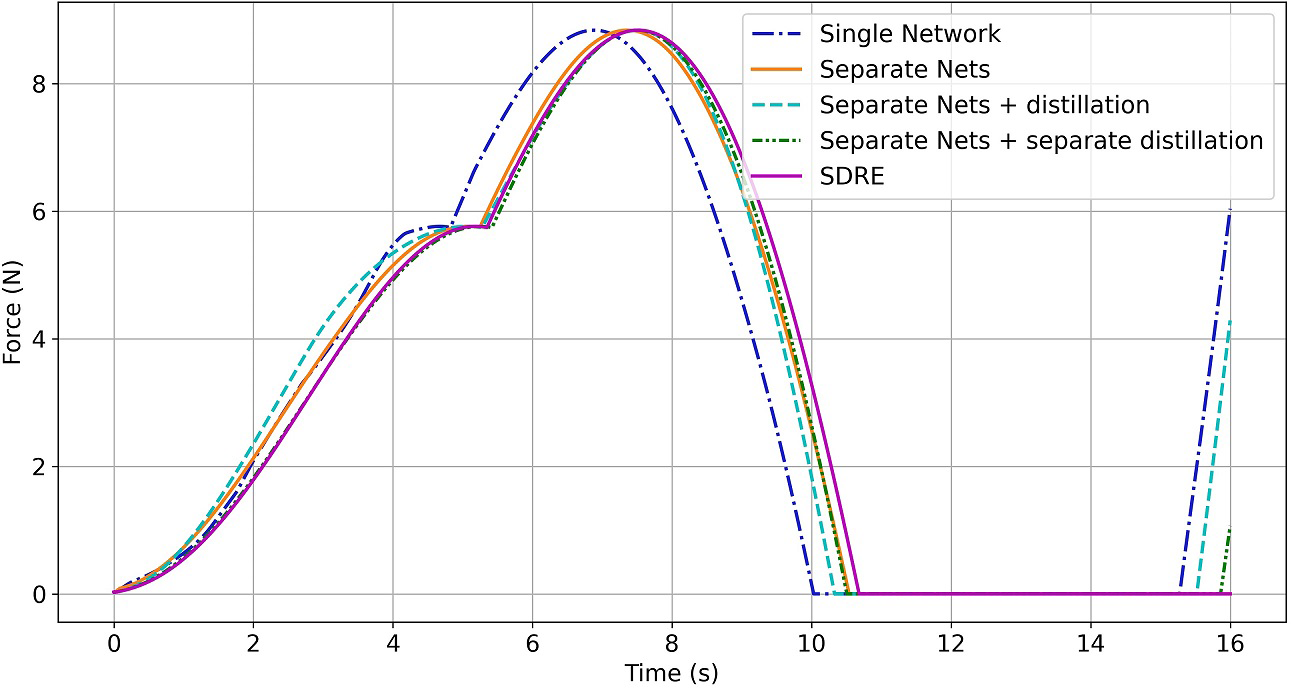
The control signals (tendon tensions) and end-effector angles, q ₁ and q ₂, for the results obtained from various neural controllers, as well as those of the model-based SDRE controller, are illustrated in Figures 5 to 9.

Figure 5.

The first tendon force (F ₁): comparison between SDRE, single and separate networks, and single and separate distilled networks.

Figure 6.

The second tendon force (F ₂): comparison between SDRE, single and separate networks, and single and separate distilled networks.

Figure 7.

The third tendon force (F ₃): comparison between SDRE, single and separate networks, and single and separate distilled networks.

Figure 8.

Continuum robot state: q ₁ (rad). Comparison between SDRE, single and separate networks, and single and separate distilled networks.

Figure 9.

Continuum robot state: q ₂ (rad). Comparison between SDRE, single and separate networks, and single and separate distilled networks.

The MSEs of angles q ₁ and q ₂ in different cases with respect to those of the SDRE controller are compared in Table 4.

Table 4.

MSE of angles.

	$q_{1} (rad)$	$q_{2} (rad)$
Case 1	0.00125	$1.01 \times 10^{- 5}$
Case 2	0.00031	$5.28 \times 10^{- 6}$
Case 3	0.00073	$8.69 \times 10^{- 6}$
Case 4	0.00025	$6.525 \times 10^{- 6}$

MSE: mean squared error.

The results in Figures 5 to 7 indicate that case (2) (two separate networks without distillation) and case (4) (two separate networks with separate distillation) perform better than other cases. Additionally, deviation from the ideal SDRE control signal is large in case (3) (two separate networks with a single distillation), although the error is greatest in case (1) (single network without distillation). As seen in Figures 8 and 9, all cases perform well for the angle q ₂. However, cases (4) and (1) perform the best and worst in terms of angle q ₁ control, respectively. Cases (2) and (4) have very similar performance, but case (4) has very fewer parameters. This result supports the claim that the distilled network can be implemented as a digital controller with a higher sampling frequency on the same hardware.

It can be interpreted that in the multi-output regression problem of CR control, it is preferable to train a network separately for each output to obtain the best performance. As well, when one network with several outputs is trained for such a problem, all of the outputs are functions of some mutual weight (i.e. the parameters of shared layers). This complicates network training. Additionally, distillation should be performed independently on each network for the same reason.

Conclusions

The present work uses neural networks with KD to replicate a powerful but computationally expensive SDRE to optimally control the challenging dynamics of CRs for the first time. While many prior efforts on CR control have focused on the kinematics of the robot, the present work employs the dynamics of the system described by the Lagrangian approach. Different setups for neural network and KD were explored in this respect, and it was found that training a separate network for each output and distilling those networks independently produced the best results for a simple CR in simulation. The comparison between the precise SDRE controller and the neural SDRE controller without KD shows that the trained distilled neural SDRE controller requires less computation. To address time-consuming and labor-intensive process of collecting and classifying data from the real world, all neural networks in this work are tuned using synthetic/simulation data. The proposed controller is applicable to all types of CRs whose models are presented using the Lagrangian technique.

Nomenclature

$q$	controllable degrees of freedom for a tendon-driven CR
q ₁	horizontal angle of the end-effector with respect to the X-axis in the XY plane
q ₂	vertical angle of the end-effector with respect to Z-axis
s	section of continuum robot
$n_{s}$	first column of the rotation matrix
$b_{s}$	second column of the rotation matrix
$t_{s}$	third column of the rotation matrix
$ω_{s}$	angular velocity of each section of arm
$J_{p} (s)$	position Jacobian matrix at section s
$ℒ$	Lagrangian of the system
$K$	kinetic energy of the system
$U$	potential energy of the system
$K_{m . b}$	kinetic energy of the main backbone
$K_{d}$	total kinetic energy of disks
$ρ_{s}$	backbone’s density
A_s	cross section area
$I_{s}$	moment of inertia matrix of section s
$I_{d}$	moment of inertia of each disk
m_d	mass of each disk
${\dot{p}}_{s}$	linear velocity of arm at section s
h	distance between disks
n	number of disks
l	length of the backbone
$U_{m . b}$	potential energy of the main backbone
$U_{d}$	potential energy of disks
g	gravity acceleration value
$e_{3}$	gravity acceleration direction
E_s	Young’s modulus of the main backbone
$u$	control signal
$F_{ten}$	tendons tensions
$x$	state vector
$e$	error vector
$Q$	positive definite weight matrices for tracking cost
$R$	positive definite weight matrices for control effort cost
$ℋ$	Hamiltonian
h	co-states
$u^{*}$	optimal control signal
$x_{e}$	input of each training sample
$K_{i}$	SDRE control gains ( $i = 1, 2$ )
$σ (.)$	activation function

Footnotes

Declaration of conflicting interests

The author(s) declared no potential conflicts of interest with respect to the research, authorship, and/or publication of this article.

Funding

The author(s) received no financial support for the research, authorship, and/or publication of this article.

ORCID iDs

Mohammadamin Samadi Khoshkho

Michael G Lipsett

References

Dupont

Lock

Itkowitz

, et al. Design and control of concentric-tube robots. IEEE Trans Robot 2010; 26(2): 209–225.

Webster

Romano

Cowan

. Mechanics of precurved-tube continuum robots. IEEE Trans Robot 2009; 25(1): 67–78.

Yip

Camarillo

. Model-less feedback control of continuum manipulators in constrained environments. IEEE Trans Robot 2014; 30(4): 880–889.

Cheng

Huang

. Design and development of a novel SMA actuated multi-DOF soft robot. IEEE Access 2019; 7: 75073–75080.

Mao

Santoso

Onal

, et al. Sim-to-real transferable object classification through touch-based continuum manipulation. In: International symposium on experimental robotics. Cham: Springer, 2020, pp. 280–289. https://doi.org/10.1007/978-3-030-33950-0_25

Guochen

Qingji

, et al. Path-tracking algorithm for aircraft fuel tank inspection robots. Int J Adv Robot Syst 2014; 11(5): 82.

Rone

Ben-Tzvi

. Continuum robotic tail loading analysis for mobile robot stabilization and maneuvering. In: International design engineering technical conferences and computers and information in engineering conference, Vol. 46360. Buffalo, New York, USA: American Society of Mechanical Engineers, p. V05AT08A009. https://doi.org/10.1115/DETC2014-34678

Samadikhoshkho

Ghorbani

Janabi-Sharifi

. Modeling and control of aerial continuum manipulation systems: a flying continuum robot paradigm. IEEE Access 2020; 8: 176883–176894.

Wang

, et al. An analytic method for the kinematics and dynamics of a multiple-backbone continuum robot. Int J Adv Robot Syst 2013; 10(1): 84.

10.

Till

Aloi

Rucker

. Real-time dynamics of soft and continuum robots based on Cosserat rod models. Int J Rob Res 2019; 38(6): 723–746.

11.

Grazioso

Di Gironimo

Siciliano

. A geometrically exact model for soft continuum robots: the finite element deformation space formulation. Soft Robot 2019; 6(6): 790–811.

12.

Godage

Webster

Walker

. Center-of-gravity-based approach for modeling dynamics of multisection continuum arms. IEEE Trans Robot 2019; 35(5): 1097–1108.

13.

Samadikhoshkho

Ghorbani

Janabi-Sharifi

. Coupled dynamic modeling and control of aerial continuum manipulation systems. Appl Sci 2021; 11(19): 9108.

14.

Thuruthel

Ansari

Falotico

, et al. Control strategies for soft robotic manipulators: a survey. Soft Robot 2018; 5(2): 149–163.

15.

Abu Alqumsan

Khoo

Norton

. Multi-surface sliding mode control of continuum robots with mismatched uncertainties. Meccanica 2019; 54(14): 2307–2316.

16.

Mousa

Khoo

Norton

. Robust control of tendon driven continuum robots. In: 2018 15th International workshop on variable structure systems (VSS), Graz, Austria, 9–11 July 2018, pp. 49–54. IEEE. DOI: 10.1109/VSS.2018.8460324

17.

Alqumsan

Khoo

Norton

. Robust control of continuum robots using Cosserat rod theory. Mech Mach Theory 2019; 131: 48–61.

18.

Kapadia

Walker

. Task-space control of extensible continuum manipulators. In: 2011 IEEE/RSJ international conference on intelligent robots and systems, San Francisco, CA, USA, 25–30 September 2011, pp. 1087–1092. IEEE.

19.

Kapadia

Walker

Dawson

, et al. A model-based sliding mode controller for extensible continuum robots. In: Proceedings of the ninth WSEAS international conference on signal processing, robotics and automation, pp. 113–120. WSEAS.

20.

Best

Gillespie

Hyatt

, et al. A new soft robot control method: using model predictive control for a pneumatically actuated humanoid. IEEE Robot Autom Mag 2016; 23(3): 75–84.

21.

Renda

Giorelli

Calisti

, et al. Dynamic model of a multibending soft robot arm driven by cables. IEEE Trans Robot 2014; 30(5): 1109–1122.

22.

Gravagne

Rahn

Walker

. Large deflection dynamics and control for planar continuum robots. IEEE/ASME Trans Mechatron 2003; 8(2): 299–307.

23.

Gravagne

Walker

. Uniform regulation of a multi-section continuum manipulator. In: Proceedings 2002 IEEE international conference on robotics and automation (Cat. No. 02CH37292), Vol. 2. Washington, DC, USA, 11–15 May 2002, pp. 1519–1524. IEEE.

24.

Wang

Kwok

. A survey for machine learning-based control of continuum robots. Front Robot AI 2021; 8: 730330.

25.

Giorelli

Renda

Ferri

, et al. A feed-forward neural network learning the inverse kinetics of a soft cable-driven manipulator moving in three-dimensional space. In: 2013 IEEE/RSJ international conference on intelligent robots and systems, Tokyo, Japan, 3–7 November 2013, pp. 5033–5039. IEEE. DOI: 10.1109/IROS.2013.6697084

26.

Giorelli

Renda

Calisti

, et al. Learning the inverse kinetics of an octopus-like manipulator in three-dimensional space. Bioinspir Biomim 2015; 10(3): 035006.

27.

Thuruthel

Falotico

Cianchetti

, et al. Learning global inverse statics solution for a redundant soft robot. In: Proceedings of the 13th international conference on informatics in control, automation and robotics ICINCO , Vol. 2, pp. 303–310. INSTICC, SciTePress, ISBN 978-989-758-198-4. DOI: 10.5220/0005979403030310

28.

Chen

Lau

, et al. Data-driven methods towards learning the highly nonlinear inverse kinematics of tendon-driven surgical manipulators. Int J Med Robot Comput Assist Surg 2017; 13(3): e1774.

29.

Bern

Schnider

Banzet

, et al. Soft robot control with a learned differentiable model. In: 2020 Third IEEE international conference on soft robotics (RoboSoft), New Haven, CT, USA, 15 May 2020–15 July 2020, pp. 417–423. IEEE. DOI: 10.1109/RoboSoft48309.2020.9116011

30.

You

Zhang

Chen

, et al. Model-free control for soft manipulators based on reinforcement learning. In: 2017 IEEE/RSJ international conference on intelligent robots and systems (IROS), Vancouver, BC, Canada, 24–28 September 2017, pp. 2909–2915. IEEE. DOI: 10.1109/IROS.2017.8206123

31.

Liu

Gasoto

Jiang

, et al. Learning to locomote with artificial neural-network and CPG-based control in a soft snake robot. In: 2020 IEEE/RSJ international conference on intelligent robots and systems (IROS), Las Vegas, NV, USA, 24 October 2020–24 January 2021, pp. 7758–7765. IEEE. DOI: 10.1109/IROS45743.2020.9340763

32.

Pearson

. Approximation methods in optimal control I. sub-optimal control. Int J Electron 1962; 13(5): 453–469.

33.

Chikhaoui

Burgner-Kahrs

. Control of continuum robots for medicalapplications: State of the art. 2018.

34.

da Costa

Saotome

Rafikova

, et al. Fast real-time SDRE controllers using neural networks. ISA Trans 2021; 118: 133–143.

35.

Hinton

Vinyals

Dean

, et al. Distilling the knowledge in a neural network, 2015. arXiv preprint arXiv:150302531.

36.

Godage

Wirz

Walker

, et al. Accurate and efficient dynamics for variable-length continuum arms: a center of gravity approach. Soft Robot 2015; 2(3): 96–106.

37.

Amouri

Mahfoudi

Zaatri

. Dynamic modeling of a spatial cable-driven continuum robot using Euler-Lagrange method. Int J Eng Technol Innov 2020; 10(1): 60–74.

38.

Kirk

. Optimal control theory: an introduction. North Chelmsford, MA, USA: Courier Corporation, 2004.

Distilled neural state-dependent Riccati equation feedback controller for dynamic control of a cable-driven continuum robot

Abstract

Keywords

Introduction

Dynamic modeling

Control design

State-dependent Riccati equation

Data acquisition and learning procedure

Simulation results

Conclusions

Nomenclature

Footnotes

Declaration of conflicting interests

Funding

ORCID iDs

References