
Abstract
The existing Bug algorithms, which are the same as wall-following algorithms, offer good performance in solving local minimum problems caused by potential fields. However, because of the odometer drift that occurs in actual environments, the performance of the paths planned by these algorithms is significantly worse in actual environments than in simulated environments. To address this issue, this article proposes a new Bug algorithm. The proposed algorithm contains a potential field function that is based on the relative velocity, which enables the potential field method to be extended to dynamic scenarios. Using the cumulative changes in the internal and external angles and the reset point of the robot during the wall-following process, the condition for state switching has been redesigned. This improvement not only solves the problem of position estimation deviation caused by odometer noise but also enhances the decision-making ability of the robot. The simulation results demonstrate that the proposed algorithm is simpler and more efficient than existing wall-following algorithms and can realise path planning in an unknown dynamic environment. The experimental results for the Kobuki robot further validate the effectiveness of the proposed algorithm.
Introduction
Mobile robots must be capable of performing autonomous navigation in unknown environments. This requires the robot to plan its motion to reach destination points while avoiding obstacles. Several methods have been proposed to address this challenge. Based on whether global information is required, path planning algorithms can be divided into two categories—global and local path planning algorithms. 1 The key precondition of global methods is the acquisition of complete and accurate prior knowledge about the environment. 2 However, the dynamic complexity, unpredictability, and real-time performance of actual application scenarios pose challenges to global path planning and navigation. By contrast, the local method only uses the robot sensors to achieve obstacle-avoidant navigation in unknown scenarios. The main methods for implementing this approach include the artificial potential field (APF) method 3 and the Bug algorithm, which is the same as the wall-following algorithm. 4
The APF method is implemented using the superposition of the attractive field generated by the target point and the repulsive force field generated by the surrounding obstacles. Under the force of a superimposed potential field, the robot can only move along the negative gradient direction of the potential field. During the movement process, the robot is pulled by the attractive force of the target and pushed by the repulsive force of the surrounding obstacles, following an effective path between the starting point and the target point. The advantages of the APF approach are its low planning complexity, fast response, and effective obstacle avoidance. 5 Because conventional methods only contain location information, it is easy for them to fall into local minima, and therefore, they can only be applied to static environments. 6
To solve the local minimum problem, Bug algorithms are becoming increasingly popular for local path planning. Bug algorithms are also known as wall-following algorithms. A Bug algorithm only needs to know the target location and not the global environment information. 7 The basic concept underlying such algorithms is the design of conditions for switching between the wall-following mode and the target approach mode. 8 The algorithm must ensure that the robot switches from the wall-following mode to the target approach mode when its distance to the target is sufficiently short to guarantee global convergence.
A certain rule in a Bug algorithm is designed based on only the local information. When the robot touches a wall, it switches to wall-following mode to bypass the obstacle. The setting of these switching rules gives Bug algorithms wider applicability. Both Bug1
9
and Bug2
10,11
firstly draw an imaginary line between the initial and target positions, called the M-line. When the robot touches a wall en route to the target, the path point is considered as the hit-point position. Then, the agent follows the border of the obstacle until it hits the same M-line on the other side of the obstacle. If that point is closer to the target than the hit-point position, then it departs from the obstacle. Zhang defined
Although the aforementioned algorithms perform well, both the M-line and
Zhu designed a new mode-switching condition. When the distance between the robot and the target began to decrease, the robot reverted to the target-approaching mode. 19 Borenstein 20 and Sanchez 21 switched states when the angle between the robot and the target was below a certain threshold. However, when the shape of the obstacle becomes complex, these switching conditions may be too simple to complete the task.
To achieve efficient and real-time path planning in an unknown dynamic environment, this article proposes an improved Bug algorithm that addresses many of the limitations of the existing APF and Bug algorithms using accumulated angle information. Based on the optimised potential field function, this method can achieve path planning in a dynamic environment. In addition, we designed a new mode-switching condition based on the relative cumulative angle and reset point, which not only alleviates the sensor noise problem but also reduces the path length (PL) in a static environment compared with some classical Bug algorithms. The results of experimentation using the Kobuki robot 22 further validate the effectiveness of the proposed algorithm.
The rest of this article is organised as follows. In the second section, the improved APF method and the wall-following algorithm are described in detail, including the APF mode, mechanism of obstacle avoidance based on wall-following algorithm and the switching mechanism between the two states. The third section not only introduces the mathematical model of the mobile robot, the simulation results on the Webots platform and the application of the algorithm in the actual environment but also discusses the convergence and stability of the algorithm in detail. In addition, the third section also compares with several traditional methods (the minimum risk method, TangentBug and Bug2). Finally, the final section represents the conclusions and future work.
Algorithm description
The new method consists of two modes, namely APF mode and wall-following mode, similar to the multiple modes employed in previous studies. 11 The two modes cyclically switch, as shown in Figure 1. The local minimum is the point at which the robot begins to swing or wander around in a cycle when the robot is in APF mode.

Switching relationship between states.
The methods of realising the two modes, as well as their switching conditions, are described in the following subsections.
APF mode
The most commonly used attractive and repulsive potentials take the following forms 24
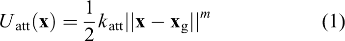

where

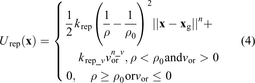

where
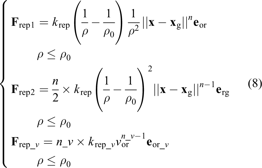
where

Relationships between unit vectors.
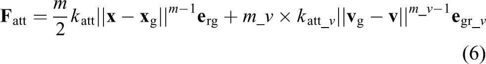
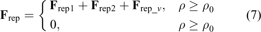
The total force applied to the robot is the sum of the attractive and repulsive forces

The enhanced potential function overcomes the poor performance of dynamic scenarios. However, the robot may stop moving or wander around the point at which the attractive force is equal to the repulsive force, which is known as the local minimum. The following switch conditions were set to identify the local minimum.
In all reported end conditions, ‘&’ denotes logical ‘AND’ and ‘|’ denotes logical ‘OR’. Condition 1 means that the superposition force tends towards zero (ε is a very small positive number), which is a common condition for judging the local minimum. However, because the system is dynamic, the robot overshoots the equilibrium position and either oscillates or wanders around in a cycle. 20 Therefore, local minima cannot be accurately identified by exclusively using condition 1 in actual environments. In condition 2, θ att and θ 0 represent the robot-to-target direction and actual instantaneous direction of travel, respectively. If the angle between the forward direction of the robot and the target direction exceeds 90°, that is, if the robot starts to move away from the target, it is likely to become trapped. Therefore, to avoid such a situation, the controller monitors condition 2. If condition 2 is satisfied, then the system switches to the recovery algorithm, as discussed in the subsequent subsections.
Wall-following mode
As shown in Figure 3, the robot starts at S and moves directly to the target at T based on the total force of the potential field. When it encounters obstacles (such as that at A), the robot continues to move along the obstacles (at A–D) under the potential field. Because of the constant change in the resultant force direction during the movement process (i.e. the resultant force in segments A–C moves to the right, whereas the resultant force in segments C–D moves to the left), the robot can accelerate, decelerate or even move back and forth between B and D. This behaviour occurs because the attractive force is equal to the repulsive force at point C, which is the local minimum. The angle between the direction of the instantaneous velocity and the attractive force at the cut-off point at C is defined as θ, which is theoretically 90°. When the robot is at C, assuming that the obstacle has been removed, the repulsive force generated by the obstacle disappears, and the robot is only affected by the attractive force. The robot direction is deflected from the original forward direction to the direction of the wall by a certain angle θ. The new forward direction is close to the attractive direction and facing the target.

Force model near local minimum. (The points A–F represent the path points, respectively.
If the robot can continue following the wall to point F, then its direction is deflected at an angle of θ in the direction of attraction. This behaviour is similar to the deflection generated by the removal of the obstacle at C. Additionally, a wall gap is located at E, which means that there is no obstacle in the forward direction of the robot. The robot believes that the obstacle has been bypassed. According to this obstacle-avoidance process, changing θ is sufficient for the robot to reach the target position.
Switching conditions were designed according to the above assumptions and analysis.
The angle of rotation of the robot under the wall-following mode to the same side of the barrier is defined as the inner angle,
Condition 1 introduces a reset point to help the robot decompose the complex environment into several simple environments. The reason for implementing this condition is that after resetting
In the previous hypothesis, the deflection angle of the velocity direction at C towards the obstacle is the same as that of the inner angle
As shown in condition 3, the vertical projection distance
An example is depicted in Figure 4. Influenced by the force field, the robot travels from S to T. According to the switching conditions of the potential field state, the robot enters the wall-following mode at A, sets the initial attitude (
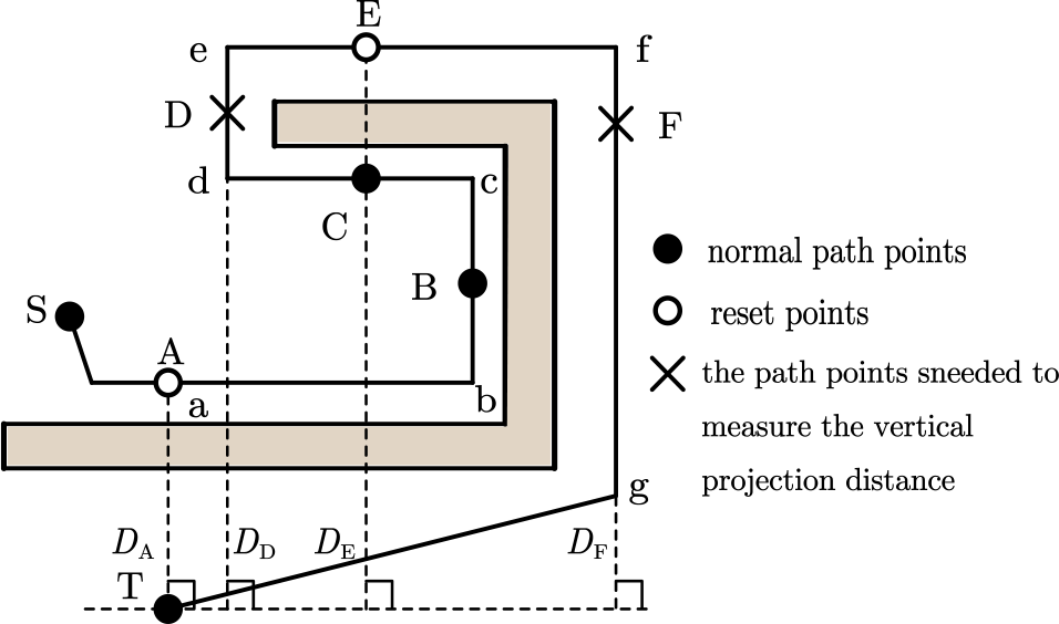
Ideal path planning in a sample environment. (The state from A to F is the same, and the state is the same in these intervals. For segment ab in the figure, the angle state within this range is the same as that of point A. In this article, we use point A to represent segment ab. The other B–F all represent the state in the corresponding line segment.)
Simulation and experimental results
Simulation model
The experimental study consisted of simulations based on Webots (Cyberbotics Ltd, Switzerland) and experiments on actual Kobuki robots. The laser sensor Rplidar A1M8 (Slamted Ltd, China) was used as the range sensor. The position of the obstacle in the Lidar coordinates can be calculated at sampling times t1 and t2. The difference between the two positions is the relative displacement between the obstacle and the robot,
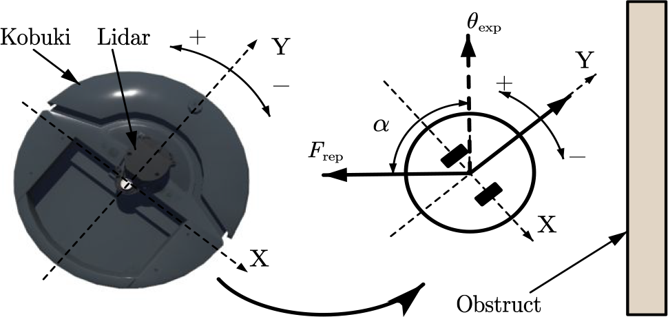
Force map for wall-following mode.
Algorithm realisation
In APF mode, at each sampling moment, the linear velocity v, angular velocity


where
In wall-following mode, v,


where
The cumulative angle is measured by a gyroscope and calculated using the following expression, where

Parameter adjustment
Parameter α affects the smoothness of the robot trajectory in wall-following mode. Considering practical application environments, the relationship between the trajectory and

Parameter influence on (a) motion trajectories and (b) expected motion angle.
The results indicate that the expected direction of motion is more inclined to the obstacle at α = 92° than at α = 90°, which leads to a trajectory that is close to the wall. Therefore, the robot needs to adjust
Simulation studies
The reset point can decompose a complex environment into a collection of simple environments. Figure 7(a) to (f) presents the six typical simple environments that were used to verify the effectiveness of the algorithm. Figure 7(a) to (d) shows an obstacle with a rectangular border, and Figure 7(e) and (f) illustrates an obstacle with an arbitrary bending angle. The experimental results indicate that a robot using the proposed algorithm can successfully plan paths in various obstacle-strewn environments with different characteristics. Therefore, path planning for any environment can be conducted by using the reset point.

Path planning in different simple environments: (a) to (d) an obstacle with a rectangular border and (e) and (f) an obstacle with an arbitrary bending angle.
Figure 8(a) depicts a complex static environment composed of typical simple environments. The robot successfully reaches the target point, which proves the validity of the reset point. There are both static and moving obstacles in the environment in Figure 8(b). After avoiding the moving obstacle, the agent starts to follow the boundary of the U-shaped obstacle and successfully reaches the static target. Spaces with moving obstacles and targets are shown in Figure 8(c) to (f). In the simulation experiment, we set the target to move for 10s at a linear velocity of 0.5 m/s and then stop. The robot moves at the linear velocity of 0.5 m/s until the moving target is reached. The starting positions of the robot and the target are the same in the scenarios depicted in Figure 8(c) and (e), but the obstacle speeds are different. In the situations illustrated in Figure 8(e) and (f), the starting position is changed without changing the environment, and consequently, the obstacle speed is different. The proposed method performed well under these conditions.

Path planning in different complex environments. (a) Environment with only static obstacles. (b) Environment with static and moving obstacles (
Stability and convergence of the algorithm
The stability of the controller is given by the Lyapunov
25
stability formula


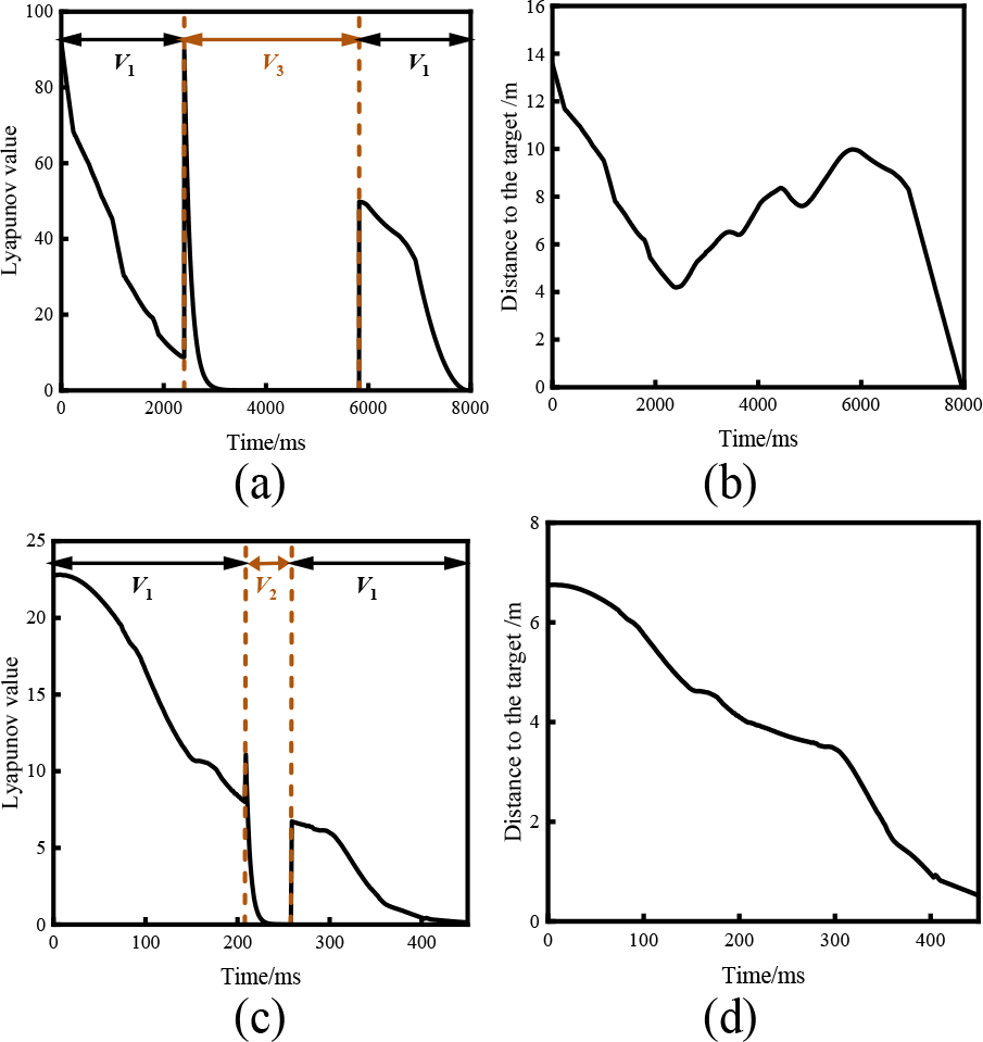
Stability and convergence of the algorithm in static and dynamic environments. (a) Stability and (b) convergence of the algorithm in a static scene. (c) Stability and (d) convergence of the algorithm in a dynamic scene.
Comparison with the minimum risk method, TangentBug and Bug2
The simulation results presented in Figure 10 illustrate the performance of the proposed method compared with those of the minimum risk method, 26 TangentBug 16 and Bug2. 11 Table 1 presents PL measurements traced by the minimum risk method, TangentBug, Bug2 and the proposed method in scenarios 1, 2 and 3, which correspond to the three scenarios in Figure 10. Wang proposed a minimum risk method based on a memory grid that records the trajectory traversed by the robot. After encountering obstacles, the robot uses the memory grid to address the local minimum problem faced by a goal-oriented robot navigating in unknown indoor environments. However, when trapped in a local minimum, the robot uses ‘trial-and-return’ behaviour to arrive at the nearest exit. Although the trial-and-return behaviour appears to be reliable in some environment, it is time consuming in U-shaped environments, as shown in Figure 10(a). The proposed method is more efficient because it uses the cumulative angle and reset point design in the switching conditions. The results of the proposed method are presented in Figure 10(b).
Path length measurements traced by the minimum risk method, TangentBug, Bug2 and the proposed method in scenarios 1, 2 and 3.


Comparison of the proposed method with some existing methods. (a) Minimum risk method in environment 1. (b) Proposed algorithm in environment 1. (c) TangentBug in environment 2. (d) Proposed algorithm in environment 2. (e) Bug2 in environment 3. (f) Proposed algorithm in environment 3.
TangentBug constructs a local tangent graph within the maximum range of the robot sensor. The agent records the distance from the local minimum to the obstacle and adds the remaining distance from that obstacle to the target. This distance is represented by
Bug2 draws an imaginary line between the beginning and end positions, called the M-line. When it touches a wall on the way to the target, the robot records the distance
Experiments on an actual robot
The proposed method was also been tested on an actual Kobuki robot (shown in Figure 11), and experiments were conducted in an indoor environment populated by various boxes. The experimental scenario is illustrated in Figure 12. Each obstacle consisted of a square box.

Kobuki robot used in the experiments.

Experimental results in an actual environment. Robot reaches the goal in: (a) a static environment and (b) an actual environment with static and dynamic obstacles.
Figure 12(a) depicts the static obstacle used in the experiment. The robot started to move from S and avoided the static obstacle by switching into wall-following mode twice (starting at A and C). At D, the robot switched back into APF mode. Finally, it reached T due to the attractive force of the target. Figure 12(b) depicts the scene containing the dynamic obstacles. The speed of both the robot and the moving obstacle was 0.3 m/s. The robot started to move from S. After avoiding moving obstacles at A, the robot started to follow the boundary of the static obstacle at B and switched from wall-following mode at C. The robot finally reached the target.
From the actual planned trajectory, it can be observed that the robot successfully bypassed obstacles in an actual complex environment and completed the path from the starting point to the target point. Comparison of the experimental results with the corresponding simulation results reveals that the two sets of results are consistent, which further verifies the feasibility of the algorithm.
Conclusion
In this study, an improved Bug method was developed to implement path planning in unknown dynamic environments, using a relative velocity to construct a new potential field function. In addition, the relative cumulative angle was recorded for the wall-following status and represented the change in the advance angle between the current attitude of the robot and its initial attitude, improving the capability of the robot to understand unknown environments. Further, a reset point was defined as the position with the same angular relationship as the initial position and was used to reset the state to the initial state to simplify the environment. By utilising the relative cumulative angle and the reset point of the new switching conditions, the robot approached the target gradually in wall-following mode under global convergence. Compared with the existing methods, which experience odometry drift, the proposed method is straightforward to implement in actual environments, making it more suitable for implementation in such environments.
The simulation results demonstrate that the proposed method can solve the local minimum problem of the potential field method by switching conditions in various environments, and it performs well in dynamic environments. Compared with the existing algorithms (minimum risk method, TangentBug and Bug2), the proposed method has a shorter PL and higher efficiency. Experiments on actual robots further verified the feasibility and applicability of the proposed algorithm.
However, this algorithm also has some limitations. First, the control structure based on condition switching makes the robot have a fast response ability and reduces the instability caused by inaccurate perception of the environment. However, direct behaviour switching makes coordination between behaviours more difficult, and occasionally unexpected situations occur. In addition, the hyperparameters set in this study were universal values applicable to most scenes. In some environments, problems such as excessive turning radii and uneven planning lines will still exist. In the future, more reasonable methods will be used to dynamically adjust the hyperparameters according to the environment.
Footnotes
Availability of data and material
Videos are provided as electronic supplementary material.
Declaration of conflicting interests
The author(s) declared no potential conflicts of interest with respect to the research, authorship, and/or publication of this article.
Funding
The author(s) disclosed receipt of the following financial support for the research, authorship and/or publication of this article: This work was supported by the National Natural Science Foundation of China under grants no. 61973159 and Science and Technology Project of Nantong City (JC22022075).
Supplemental material
Supplemental material for this article is available online.
References
Supplementary Material
Please find the following supplemental material available below.
For Open Access articles published under a Creative Commons License, all supplemental material carries the same license as the article it is associated with.
For non-Open Access articles published, all supplemental material carries a non-exclusive license, and permission requests for re-use of supplemental material or any part of supplemental material shall be sent directly to the copyright owner as specified in the copyright notice associated with the article.