Sage Journals: Discover world-class research

Abstract

Modeling and analysis of inverse kinematics and dynamics for a novel parallel manipulator are established in this article. The manipulator is a spatial mechanism, which consists of six identical kinematic chains connecting to the moving platform. Firstly, screw theory is applied to compute the degree of freedom of this manipulator. Then the inverse position is achieved based on the homogeneous coordinate transformation principle while motion law of the moving platform is given. Furthermore, the first-order influence coefficient method is employed to obtain the Jacobian matrices of the considered manipulator and the links, so do the velocities. Afterward, the rigid-body dynamics model is derived from the Lagrange formulation. To obtain the integrated inverse dynamics model, an approach for simplified flexible dynamics analysis is proposed. Finally, simulations are conducted to compute the position and driving force of this considered manipulator, which validate the new method simultaneously.

Keywords

Parallel manipulator kinematics dynamics influence coefficient Lagrange formulation

Introduction

A multi-degree of freedom mechanism is needed to support the aircraft models in the wind tunnel tests. In practice, an aircraft model will move along the given trajectory, which usually contains pitch, roll, yaw, heave, surge, and sway motion about the reference coordinate system, so a kind of 6-DOF mechanisms with high precision and stabilization are required to achieve the demands of corresponding tests.^1,2 Parallel manipulators are closed-loop mechanical structures composed of a moving platform coupled to a fixed base by serial limbs, which usually can provide multi-degree of freedom with great comprehensive performance,^3,4 and they will be a good choice for wind tunnel tests.

Kinematics and dynamics analysis are fundamental research of parallel manipulators. With regards to kinematics analysis, it has been extensively studied in literature. Araujo-Gómez et al.⁵ designed a 2R2T parallel manipulator and put forward the kinematics equations of the manipulator in accordance with the anchoring points coordinates. Zarkandi⁶ introduced a novel flight simulator manipulator with four degrees of freedom, while kinematic analysis and workspace optimization are discussed in detail. Fomin et al.⁷ focused on the inverse and forward kinematic analysis of a novel parallel manipulator with a circular guide. Xu et al.⁸ proposed a new redundantly actuated parallel manipulator, and the inverse displacement solution, velocity, and singularity analyses are presented. Nayak et al.⁹ dealt with the kinematic analysis of a series–parallel manipulator, which is a minimal octic univariate polynomial with four quadratic factors. Fang et al.¹⁰ designed a new spindle parallel manipulator, and the kinematic mapping between the considered manipulator and its nonredundantly actuated forms are analyzed mathematically. Leal-Naranjo et al.¹¹ presented a spherical parallel manipulator for a prosthetic wrist, and the inverse position problem is solved in a closed form. Chen et al.¹² established the kinematic model of a spherical parallel manipulator, which is validated by a numerical example.

Sufficient efforts also have been committed to dynamics analysis of parallel manipulators. Thomas et al.¹³ investigated the dynamics of a spatial parallel manipulator, and the model is presented using the Euler–Lagrangian approach with Lagrangian multipliers to include the system constraints. Pedrammehr et al.¹⁴ establish a closed-form model for dynamics analysis, which is based on the principle of virtual work. Chen et al.¹⁵ employed the Newton–Euler formulation with generalized coordinates to establish the dynamics model of a 1T2R parallel manipulator. Gallardo-Alvarado et al.¹⁶ reported a Schönflies parallel manipulator, and the dynamic model is built resorting to the combination of screw theory and virtual work. Based on the flexible multi-body dynamics theory, Liang et al.¹⁷ developed the rigid-flexible coupling dynamics model by virtue of the augmented Lagrangian multipliers approach. Korayem and Dehkordi¹⁸ provided the dynamic equations of a flexible cooperative manipulator, which was derived using the recursive Gibbs–Appell formulation. Zheng et al.¹⁹ established a dynamics model of a flexible linkage mechanism using virtual joint velocities, restraint force impulses, and gauge momentum derivatives. Wang and Wang²⁰ built a high-fidelity dynamics model of a spatial parallel mechanism, the model considered the flexible moving platform and the clearance spherical joint.

One of the objectives of this work is to analyze the kinematic characteristic of the considered parallel manipulator, especially the mobility and velocity properties. Note that, most approaches for mobility analysis can only compute the number of degree of freedom but cannot reveal the property of the mobility. Moreover, traditional methods for velocity analysis are very complicated. Therefore, it will be of great significance to employ a simple and effective method to analyze the manipulator’s kinematic characteristic. As with flexible dynamics, if the whole mechanical system is taken into flexible processing, the procedure of calculation and simulation will be very complex and difficult. Hence, another objective of this work is to put forward a simplified method for the analysis of flexible dynamics.

In this article, a 6-PSU parallel manipulator is put forward to sustain the wind tunnel tests. As with its complicated spatial structure, the analysis of kinematics and dynamics is not so easy to conduct. So the first-order influence coefficient method is applied to obtain the inverse kinematics equations, and a novel method is proposed to achieve the integrated inverse dynamics model. In the meantime, simulation examples carried out by Matlab and Adams are utilized to verify the correctness of the proposed method.

The rest of this article is organized as follows. Structure description and calculation of the degree of freedom of the considered parallel manipulator are presented in the second section. Inverse position analysis is discussed in the third section. Analysis of velocities of the sliders and struts is provided in the fourth section. The inverse dynamics model is established in the fifth section. Simulation of the rigid-body dynamics and simplified flexible dynamics are conducted in the sixth section, followed by conclusions in the seventh section.

A 6-DOF parallel manipulator

Manipulator description

Having a closed-loop structure, the 6-PSU parallel manipulator is a special symmetrical mechanism composed of six kinematic chains with identical topology, all connecting the moving platform to the base platform. As shown in Figures 1 and 2, the topology of each of the six kinematic chains is made up of a slider driven by a linear motor and a strut with a fixed length from spherical joint B to universal joint U.

Figure 1.

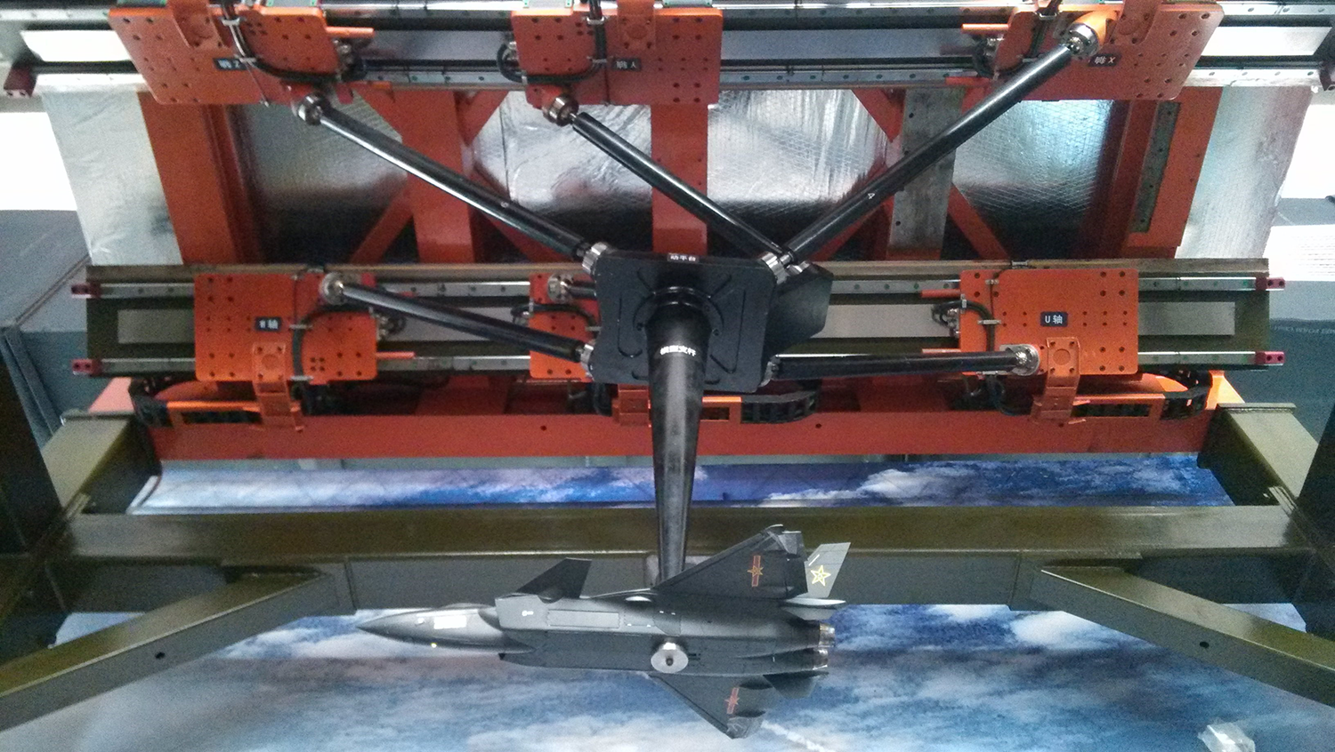
The 6-DOF parallel manipulator.

Figure 2.

Schematic diagram of the parallel manipulator.

For the purpose of analysis, the global coordinate system is attached to the fixed base with its origin located at the center O_b of the base platform, O_bX_b-axis is parallel to B₁B₂ and O_bZ_b-axis perpendicular to the base. The local coordinate system is established at the moving platform with its origin located at the center O₀ of the aircraft model. The geometric parameters of this mechanism are as shown in Figures 2 and 3 and Table 1.

Figure 3.

X-axis view of the base platform.

Table 1.

Geometric parameters.

Parameter	Value
$θ$ tilt angle between the rails and horizontal plane	30°
$ϕ$ intersection angle between plane U₂U₃U₆ and plane U₁U₃U₆	45°
d ₁ half of the distance between left and right rail	267 mm
d ₂ distance between B₆ and B₄(B₅) along the width direction of rail plane	198 mm
d ₃ half of the distance between U₁(U₃) and U₄(U₆)	115 mm
d ₄ half of the distance between U₂ and U₅	46 mm
d ₅ half of the distance between U₁(U₄) and U₃(U₆)	170 mm
d ₆ distance between U₂(U₅) and U₃(U₆)	145 mm
h initial distance between the local coordinate system and the global coordinate system	1423 mm
h ₁ distance between B₁(B₂, B₄, B₅) and the rail plane	55 mm
h ₂ distance between B₃(B₆) and the rail plane	55 mm
h ₃ distance between O₀ and Q	838 mm
l_i length of the i-th strut

Mobility analysis

As well know, it’s difficult to analyze the degree of freedom of some complicated spatial mechanisms by traditional method, so screw theory and modified Kutzbach–Grübler criterion are applied to deal with this problem.

According to screw theory,^21,22 a screw can be expressed as

$ = {[s; s_{0}]}^{T}

where s represent the direction ratio pointing along the screw axis, s ₀ = r×s is the moment of the screw axis with respect to the origin of the coordinate system, and r denotes the position vector of a chosen point on the screw axis.

Since all the six kinematic chains have identical topology, just take the first kinematic chain PSU as an example. Here, another local coordinate system o-xyz is attached to spherical joint B₁.

As described in Figure 4, complex joints can be replaced by some basic joints with a single degree of freedom, such as $S \equiv \bar{R R R}$ , $U \equiv \bar{R R}$ . Then all the kinematic joints can be represented by screws, where the prismatic joint is denoted by $$_{1}$ , the spherical joint is represented by $$_{2}$ , $$_{3}$ , and $$_{4}$ , and the universal joint is indicated by $$_{5}$ and $$_{6}$ . Hence, the kinematic screw system of the first limb under this local coordinate system can be expressed as

$^{w} = [\begin{matrix} $_{1} & $_{2} & $_{3} & $_{4} & $_{5} & $_{6} \end{matrix}]

Figure 4.

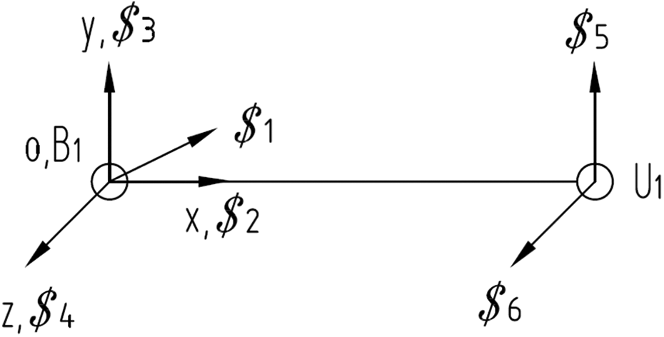
Kinematic chain of PSU.

The screws among the equation above are

\begin{array}{l} $_{1} = {[\begin{matrix} 0 & 0 & 0 & ; & a_{1} & b_{1} & c_{1} \end{matrix}]}^{T} \\ $_{2} = {[\begin{matrix} 1 & 0 & 0 & ; & 0 & 0 & 0 \end{matrix}]}^{T} \\ $_{3} = {[\begin{matrix} 0 & 1 & 0 & ; & 0 & 0 & 0 \end{matrix}]}^{T} \\ $_{4} = {[\begin{matrix} 0 & 0 & 1 & ; & 0 & 0 & 0 \end{matrix}]}^{T} \\ $_{5} = {[\begin{matrix} 0 & 1 & 0 & ; & a_{5} & 0 & 0 \end{matrix}]}^{T} \\ $_{6} = {[\begin{matrix} 0 & 0 & 1 & ; & 0 & b_{6} & 0 \end{matrix}]}^{T} \end{array}

where a ₁, a ₅, b ₁, b ₆, and c ₁ are determined by the geometry dimension of the first limb.

It’s easy to observe that the reciprocal screw of equation (3) is 0, as reciprocal screws of different chains are distinctive, so common constraint $λ = 0$ , namely this mechanism is still a six-order screw system. According to the modified Kutzbach–Grübler criterion,^23,24 over constraints and passive degree of freedom need to be taken into consideration when calculating the degree of freedom

M = d (n - g - 1) + \sum_{i = 1}^{g} f_{n} + v - ζ

M is the number of degree of freedom of the mechanism, d stands for the order of the mechanism, n is the total number of components, g represents the amount of kinematic pairs, f_n is the degree of freedom of the i-th kinematic pair, v denotes the amount of redundant constraints, and $ζ$ represents the passive degree of freedom. For this mechanism, $d = 6 - λ = 6$ , $n = 14$ , $g = 18$ , $v = 0$ , $ζ = 0$ . Then it’s calculated that $M = 6$ , namely the degree of freedom of the parallel manipulator is 6, namely three translations and three rotations, which corresponds with the actual situation.

Inverse position analysis

The inverse position problem involves mapping a known pose of the moving platform to the input of each kinematic chain. For the considered manipulator, the prismatic joint in each kinematic chain is actuated, thus the inverse position problem is to obtain the displacement of each prismatic joint.

With regard to the universal joints, their coordinates in the local frame can be obtained directly obtained from the geometric relationship:

\begin{array}{l} U_{1} = {(\begin{matrix} d_{5} & - d_{3} & - h_{3} \end{matrix})}^{T} \\ U_{2} = {(\begin{matrix} - d_{5} - d_{6} c φ & - d_{4} & - h_{3} - d_{6} s φ \end{matrix})}^{T} \\ U_{3} = {(\begin{matrix} - d_{5} & - d_{3} & - h_{3} \end{matrix})}^{T} \\ U_{4} = {(\begin{matrix} d_{5} & d_{3} & - h_{3} \end{matrix})}^{T} \\ U_{5} = {(\begin{matrix} - d_{5} - d_{6} c φ & d_{4} & - h_{3} - d_{6} s φ \end{matrix})}^{T} \\ U_{6} = {(\begin{matrix} - d_{5} & d_{3} & - h_{3} \end{matrix})}^{T} \end{array}

where c represents cosine, and s stands for sine.

Spherical joints along the YZ direction in the global coordinate system have their location coordinate that also can be obtained easily, only the x-coordinate is difficult to acquire

\begin{array}{l} B_{1} = {(\begin{matrix} x_{1} & - d_{1} + h_{1} s θ & h_{1} c θ \end{matrix})}^{T} \\ B_{2} = {(\begin{matrix} x_{2} & - d_{1} + h_{1} s θ & h_{1} c θ \end{matrix})}^{T} \\ B_{3} = {(\begin{matrix} x_{3} & - d_{1} + h_{2} s θ - d_{2} c θ & d_{2} s θ + h_{2} c θ \end{matrix})}^{T} \\ B_{4} = {(\begin{matrix} x_{4} & d_{1} - h_{1} s θ & h_{1} c θ \end{matrix})}^{T} \\ B_{5} = {(\begin{matrix} x_{5} & d_{1} - h_{1} s θ & h_{1} c θ \end{matrix})}^{T} \\ B_{6} = {(\begin{matrix} x_{6} & d_{1} - h_{2} s θ + d_{2} c θ & d_{2} s θ + h_{2} c θ \end{matrix})}^{T} \end{array}

As with this parallel manipulator, the six prismatic joints coincide with the six spherical joints, respectively. Hence, the inverse kinematics is to derive the variation of each slider along X direction, namely determine the value of x_i .

The transformation matrix from local coordinate system to global coordinate system is defined by the parameters of roll, pitch, yaw angles, and translations. Namely, a rotation of α about the X_b -axis, followed a rotation of $β$ about the Y_b -axis, a rotation of $γ$ about the Z_b -axis and X, Y, Z are the translation along the corresponding axis

T_{m} = [\begin{matrix} c β c γ & s α s β c γ - c α s γ & s α s γ + c α s β c γ & X \\ c β s γ & s α s β s γ + c α c γ & - s α c γ + c α s β s γ & Y \\ - s β & s α c β & c α c β & Z \\ 0 & 0 & 0 & 1 \end{matrix}]

According to RPY transformation, the coordinates of universal joints in the global coordinate system can be expressed as follows

U_{i}^{b} = T_{m} U_{i} (i = 1, 2, ..., 6)

The length of the struts is fixed, and the length formula is given as below

l_{i} = ‖ U_{i}^{b} - U_{i} ‖ (i = 1, 2, ..., 6)

While $l_{1} = l_{3} = l_{4} = l_{6} = 900 mm$ and $l_{2} = l_{5} = 720

mm$ , then the solution to the inverse position problem can be expressed as follows

{\begin{array}{l} x_{i} = B_{i x} = U_{i x}^{b} + \sqrt{l_{i}^{2} - {(U_{i y}^{b} - B_{i y})}^{2} - {(U_{i z}^{b} - B_{i z})}^{2}} (i = 1, 2, 4, 5) \\ x_{i} = B_{i x} = U_{i x}^{b} - \sqrt{l_{i}^{2} - {(U_{i y}^{b} - B_{i y})}^{2} - {(U_{i z}^{b} - B_{i z})}^{2}} (i = 3, 6) \end{array}

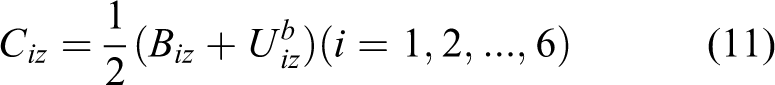
To calculate the total potential energy for dynamics analysis, the coordinates of the mass center of the struts along Z direction should be obtained, which can be written as

C_{i z} = \frac{1}{2} (B_{i z} + U_{i z}^{b}) (i = 1, 2, ..., 6)

In this section, the inverse position problem is solved by the principle of homogeneous coordinate transformation. Inverse position analysis is the basis of kinematic analysis and will be useful for dynamics analysis.

Velocity analysis

In this section, the velocity analysis of the proposed parallel manipulator under study is approached using the theory of first-order influence coefficient.

As with complex joints, they can be replaced by some basic joints, so the kinematic sketch of the first kinematic chain can be described as Figure 5. $S_{1}^{1}$ is the axis of the prismatic joint, spherical joint B₁ is substituted by three revolute joints, and $S_{2}^{1}$ , $S_{3}^{1}$ , $S_{4}^{1}$ are their axes. In a similar way, universal joint U₁ is equivalent to two intersecting revolute joints $S_{5}^{1}$ , $S_{6}^{1}$ . Assuming that $S_{1}^{1}$ and $S_{2}^{1}$ are parallel to X_b, $S_{4}^{1}$ pointing to the length direction of the strut B₁U₁, $S_{6}^{1}$ is parallel to U₁O₀. In what follows, $S_{3}^{1}$ perpendicular to $S_{2}^{1}$ and $S_{4}^{1}$ , and $S_{5}^{1}$ is normal to $S_{4}^{1}$ and $S_{6}^{1}$ . What is more, all of these vectors are unit vectors which can be described as follows

\begin{array}{l} S_{1}^{1} = {(\begin{matrix} 1 & 0 & 0 \end{matrix})}^{T} \\ S_{2}^{1} = {(\begin{matrix} 1 & 0 & 0 \end{matrix})}^{T} \\ S_{3}^{1} = S_{2}^{1} \times S_{4}^{1} \\ S_{5}^{1} = S_{4}^{1} \times S_{6}^{1} \\ S_{4}^{1} = {(\begin{matrix} \frac{U_{1 x}^{b} - B_{1 x}}{l_{1}} & \frac{U_{1 y}^{b} - B_{1 y}}{l_{1}} & \frac{U_{1 z}^{b} - B_{1 z}}{l_{1}} \end{matrix})}^{T} \\ S_{6}^{1} = {(\begin{matrix} \frac{O_{0 x}^{b} - U_{1 x}^{b}}{\bar{U_{1} O_{0}}} & \frac{O_{0 y}^{b} - U_{1 y}^{b}}{\bar{U_{1} O_{0}}} & \frac{O_{0 z}^{b} - U_{1 z}^{b}}{\bar{U_{1} O_{0}}} \end{matrix})}^{T} \end{array}

Figure 5.

Kinematic sketch of the first kinematic chain.

Velocities of the sliders

As with general parallel manipulators, they are composed of a few kinematic chains, each limb can be treated as a serial manipulator, and the motion of the moving platform can be represented as follows

V_{m} = {[G_{ϕ}^{m}]}^{(i)} {\dot{ϕ}}^{i} (i = 1, 2, ..., 6)

where $V_{m} = {[\begin{matrix} v_{m}^{T} & w_{m}^{T} \end{matrix}]}^{T}$ , v_m is the linear velocity of the chosen reference point on the moving platform, w_m is the angular velocity of the moving platform, and ${\dot{ϕ}}^{i} \in 6 x 1$ represent the velocities of all links in each limb. Moreover, ${[G_{ϕ}^{m}]}^{(i)}$ is the first-order influence coefficient matrix, and it can be expressed as

{[G_{ϕ}^{m}]}^{(1)} = [\begin{matrix} {[G_{ϕ}^{(h)}]}^{1} \\ {[G_{ϕ}^{p}]}^{1} \end{matrix}] = [\begin{matrix} 0 & S_{2}^{1} & S_{3}^{1} & S_{4}^{1} & S_{5}^{1} & S_{6}^{1} \\ S_{1}^{1} & S_{2}^{1} \times (O_{0} - R_{2}) & S_{3}^{1} \times (O_{0} - R_{3}) & S_{4}^{1} \times (O_{0} - R_{4}) & S_{5}^{1} \times (O_{0} - R_{5}) & S_{6}^{1} \times (O_{0} - R_{6}) \end{matrix}]

where R_i respects the position vector of the coordinate origin of the i-th link. If matrix ${[G_{ϕ}^{m}]}^{(i)}$ is nonsingular, its inverse matrix can be obtained ${[G_{ϕ}^{m}]}^{(i)} = {[G_{m}^{ϕ}]}^{- 1 (i)}$ .

The motion of the moving platform is given, then the velocity of the moving platform can be achieved by taking the derivative of the motion formula with respect to time. In what follows, the velocities of all links in each limb can be expressed as

{\dot{ϕ}}^{i} = {(\begin{matrix} {\dot{ϕ}}_{1}^{i} & {\dot{ϕ}}_{2}^{i} & {\dot{ϕ}}_{3}^{i} & {\dot{ϕ}}_{4}^{i} & {\dot{ϕ}}_{5}^{i} & {\dot{ϕ}}_{6}^{i} \end{matrix})}^{T} = {[G_{m}^{ϕ}]}^{(i)} V_{m}

With respect to this 6-DOF parallel manipulator, the velocity of each slider is

{\dot{ϕ}}_{1}^{i} = {[G_{m}^{ϕ}]}_{1 :}^{(i)} V_{m} (i = 1, 2, ..., 6)

where ${[G_{m}^{ϕ}]}_{1 :}^{(i)}$ represents the first row of matrix ${[G_{m}^{ϕ}]}^{(i)}$ , and ${[G_{m}^{ϕ}]}_{1 :}^{T (i)}$ is its transposed matrix.

Based on the analysis above, the relationship between the input and output velocities named Jacobian matrix can be obtained, which can be expressed as

J = {(\begin{matrix} {[G_{m}^{ϕ}]}_{1 :}^{T (1)} & {[G_{m}^{ϕ}]}_{1 :}^{T (2)} & {[G_{m}^{ϕ}]}_{1 :}^{T (3)} & {[G_{m}^{ϕ}]}_{1 :}^{T (4)} & {[G_{m}^{ϕ}]}_{1 :}^{T (5)} & {[G_{m}^{ϕ}]}_{1 :}^{T (6)} \end{matrix})}^{T}

Velocities of struts

The velocity of the k-th link in the i-th kinematic chain is

V_{k}^{i} = (\begin{matrix} v_{k}^{i} \\ w_{k}^{i} \end{matrix}) = {(\begin{matrix} v_{k x}^{i} & v_{k y}^{i} & v_{k z}^{i} & w_{k x}^{i} & w_{k y}^{i} & w_{k z}^{i} \end{matrix})}^{T}

The corresponding first-order influence coefficient matrix can be written as

{[G_{ϕ}^{K}]}^{(i)} = [\begin{matrix} {[G_{ϕ_{}}^{k h}]}^{(i)} \\ {[G_{ϕ_{}}^{k p}]}^{(i)} \end{matrix}]

with

{[G_{ϕ}^{k h}]}^{(i)} = (\begin{matrix} 0 & S_{2}^{i} & \dots & S_{k}^{i} \end{matrix})

{[G_{ϕ}^{k p}]}^{(i)} = (\begin{matrix} S_{1}^{i} & S_{2}^{i} \times (P_{i} - R_{2}) & \dots & S_{k}^{i} \times (P_{i} - R_{k}) \end{matrix})

where P_i respects the position vector of the mass center of the i-th link.

Since the sequence number of the strut is four, so the velocity of the strut is

V_{4}^{i} = {[G_{ϕ}^{K}]}^{(i)} {[G_{m}^{ϕ}]}_{1 k :}^{- 1 (i)} V_{m} (i = 1, 2, ..., 6)

In this section, the velocities of the sliders and struts are obtained by the theory of first-order influence coefficient. Velocity analysis is the basis for dynamics analysis, especially for the computation of kinetic energy.

Inverse dynamics model

Once the velocities of all components of the manipulator are obtained, the Lagrange formulation can be employed to derive the dynamics model. In the context of real-time control, neglecting the friction forces and considering the gravitational effect, and all components are assumed to be rigid bodies.

Kinetic energy

Generally, kinetic energy k is a property of a moving object or particle and depends not only on its motion but also on its mass, which can be divided into two terms as

k = k_{T} + k_{R}

where k_T represents the translational kinetic energy which is generated by translational motion, k_R denotes the rotational kinetic energy derives from rotational motion, and we have

k_{T} = \frac{1}{2} m v^{T} v

k_{R} = \frac{1}{2} w^{T} J_{c}^{o} w

where m, v, w, and $J_{c}^{o}$ are the mass, the linear velocity, the angular velocity, and the centroidal inertia tensor, respectively.

The centroidal inertia tensor can be described in another form as

J_{c}^{o} = T^{T} J_{c} T

with

J_{c} = [\begin{matrix} J_{x x} & 0 & 0 \\ 0 & J_{y y} & 0 \\ 0 & 0 & J_{z z} \end{matrix}]

where T is the transformation matrix from the reference coordinate system to the global coordinate system, and J_c is the principal moment of inertia.

The total kinetic energy of the considered parallel manipulator is composed of three main parts, namely kinetic energy of the moving platform, the sliders, and the struts. With regard to the moving platform, its kinetic energy can be described as

k_{m} = \frac{1}{2} (m_{m} v_{m}^{T} v_{m} + w_{m}^{T} J_{m}^{o} w_{m})

where $J_{m}^{o} = T_{m}^{T} J_{m} T_{m}$ .

The sliders only translate along the rails, which means their rotational kinetic energy are equal to zero, therefore the kinetic energy of the i-th slider can be expressed as

k_{i}^{s} = \frac{1}{2} m_{i}^{s} {({\dot{ϕ}}_{1}^{i})}^{2} (i = 1, 2, ..., 6)

As for the strut, the kinetic energy can be described as

k_{i}^{l} = \frac{1}{2} (m_{i}^{l} v_{4}^{T i} v_{4}^{i} + w_{4}^{T i} J_{4}^{i o} w_{4}^{i}) (i = 1, 2, ..., 6)

where $J_{4}^{i o} = T_{4}^{T i} J_{4}^{i} T_{4}^{i}$ , and $T_{4}^{i}$ is the transformation matrix from the strut in the i-th limb to the global coordinate system.

Take the first kinematic chain described in Figure 4 as an example, $T_{4}^{1}$ denotes the transformation matrix from the local coordinate system O₁-X₁Y₁Z₁ to the global coordinate system. X₁-axis is parallel to $S_{4}^{1}$ , Z₁-axis is parallel to $S_{3}^{1}$ , and i, k, j are the unit vectors along axes X₁, Y₁, Z₁, respectively, then $T_{4}^{1}$ can be addressed from following equation

{\begin{array}{l} i = T_{4}^{1} \cdot {(\begin{matrix} 1 & 0 & 0 \end{matrix})}^{T} \\ j = \frac{1}{‖ i \times S_{1}^{1} ‖} i \times S_{1}^{1} = T_{4}^{1} \cdot {(\begin{matrix} 0 & 1 & 0 \end{matrix})}^{T} \\ k = i \times j = T_{4}^{1} \cdot {(\begin{matrix} 0 & 0 & 1 \end{matrix})}^{T} \end{array}

Based on the analysis above, for the considered parallel manipulator, the total kinetic energy can be expressed as

K = k_{m} + \sum_{i = 1}^{6} k_{i}^{s} + \sum_{i = 1}^{6} k_{i}^{l}

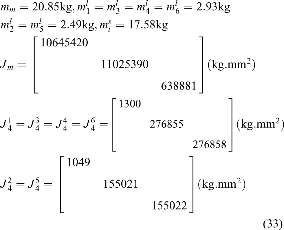
For the purpose of dynamic simulation, put the inertial parameters of this manipulator as follows

\begin{array}{l} m_{m} = 20.85 kg, m_{1}^{l} = m_{3}^{l} = m_{4}^{l} = m_{6}^{l} = 2.93 kg \\ m_{2}^{l} = m_{5}^{l} = 2.49 kg, m_{i}^{s} = 17.58 kg \\ J_{m} = [\begin{matrix} 10645420 \\ 11025390 \\ 638881 \end{matrix}] (kg {.mm}^{2}) \\ J_{4}^{1} = J_{4}^{3} = J_{4}^{4} = J_{4}^{6} = [\begin{matrix} 1300 \\ 276855 \\ 276858 \end{matrix}] (kg {.mm}^{2}) \\ J_{4}^{2} = J_{4}^{5} = [\begin{matrix} 1049 \\ 155021 \\ 155022 \end{matrix}] (kg {.mm}^{2}) \end{array}

Potential energy

Potential energy is related to the chosen coordinate system. Here, the horizontal plane of the global coordinate system is selected as the potential energy zero plane. In this way, the potential energy of each body can be obtained by considering the variation of the position of its center of mass with respect to the Z_b -axis.

Since the sliders always move in the horizontal plane, so the potential energy of the sliders are constants that will not appear in the Lagrange formulation. The potential energy for the moving platform and the struts can be described, respectively, as below

p_{m} = m_{m} g Z

p_{i}^{l} = m_{i}^{l} g C_{i z} (i = 1, 2, ..., 6)

The total potential energy of the considered manipulator is the addition of the potential energy of the struts and moving platform, which can be expressed as

P = p_{m} + \sum_{i = 1}^{6} p_{i}^{l}

Dynamics model

Since the total kinetic energy K and total potential energy P of the considered manipulator have been obtained, the Lagrange function L and the Lagrange formulation would be given as below

L = K - P

F_{i} = \frac{d}{d t} \frac{\partial L}{\partial {\dot{q}}_{i}} - \frac{\partial L}{\partial q_{i}} (i = 1, 2, ..., n)

where q_i , ${\dot{q}}_{i}$ , and F_i are the generalized coordinate, velocity, and force, respectively, and n is the total number of the limbs.

By the principle of virtual work, driving forces of the sliders can be concluded as

f = {(\begin{matrix} f_{1} & f_{2} & f_{3} & f_{4} & f_{5} & f_{6} \end{matrix})}^{T} = {[J^{T}]}^{- 1} F

where J is the Jacobian matrix of the considered manipulator which can be obtained by equation (17).

In this section, kinetic energy and potential energy of the moving platform, sliders, and struts are analyzed, based on which the total kinetic energy and potential energy of the considered parallel manipulator are obtained. Subsequently, the driving forces of the manipulator are addressed by approaches of Lagrange formulation and virtual work. The establishment of the dynamics model will be helpful for dynamics analysis.

Simulation

Simulation of the rigid-body dynamics

Generally, simulation of rigid-body dynamics could meet the requirements of the most mechanical system. Then the simulation is implemented using Matlab to solve the inverse kinematics and dynamics of this parallel manipulator. To validate the numerical model, the calculated results are compared with the ones conducted by Adams.

Based on the typical operation conditions, the following example is chosen to illustrate the algorithm. It’s assumed that there are no external force and moment exerting on the aircraft, and the aircraft only carries out pure-pitching movement while all the other positional parameters are equal to zero which can be assigned as

β = \frac{π}{12} sin (2 π t)

As graphically sketched in Figures 6 to 9, L_i and F_i denote the displacement and driving force of the i-th slider, respectively, and the comparison results of the driving force of the first slider simulated by Matlab and Adams are listed in Table 2, then following conclusions are obtained by comprehensive analysis.

Displacements and driving forces of the six sliders vary approximately sinusoidal with time, which are basically in accordance with the motion law of the aircraft. Moreover, the displacement diagrams of the sliders simulated by Matlab basically agree well with the ones conducted by Adams, which validates the correctness of the numerical model.

It is found that L ₁, L ₂, and L ₃ coincide with L ₄, L ₅, and L ₆, respectively. This phenomenon depends not only on the manipulator’s geometric construction but also on the motion law of the aircraft. As shown in Figure 2, the considered manipulator has a symmetrical geometric construction. Moreover, the pure-pitching movement means that the axis of revolution of the aircraft is perpendicular to the symmetry plane. Therefore, the displacements of the sliders at the same position on the respective rails are the same. Noted that, a similar phenomenon can be found for the driving forces.

As described in Table 2, the maximum absolute error of driving force between the two simulation software is up to 5.1%. A series of reasons leading to this error, with respect to Lagrange formulation, the friction force is ignored which will affect the simulation result conducted by Matlab. In this mechanical system, the friction coefficients of the spherical joints and universal joints are about 0.003, which will have a slight influence on the result. Then the parameters inputted are ideal, even the size of the components may do a certain effect on the simulation result, and so do the distribution of the weight. It’s assumed that Lagrange formulation could be a perfect approach to address dynamics problems if the friction coefficients and other related parameters are comparatively ideal.

Figure 6.

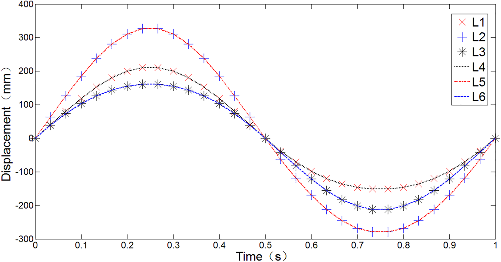
Curves of displacement within Matlab.

Figure 7.

Curves of displacement within Adams.

Figure 8.

Curves of driving force within Matlab.

Figure 9.

Curves of driving force within Adams.

Table 2.

Comparisons of driving force simulation between Matlab and Adams.

Time (s)	0	0.1	0.2	0.3	0.4	0.5	0.6	0.7	0.8	0.9	1.0
Simulation by Matlab (N)	45.45	260.30	426.36	426.36	260.31	45.45	−62.41	−49.40	−49.40	−62.41	45.45
Simulation by Adams (N)	43.30	251.76	416.94	418.02	251.25	43.52	−65.57	−47.36	−47.06	−65.50	43.59
Absolute error (%)	4.7	3.3	2.2	1.7	3.5	4.2	5.1	4.1	4.7	5.0	4.1

Simulation of the simplified flexible dynamics

As with wind tunnel experiments, high accuracy of the mechanical system is in demand, so it may not meet the designed requirement if only take rigid-body dynamics into consideration. On the other hand, the procedure of calculation and simulation will be very complex and difficult if take the whole mechanical system into flexible processing. In this section, a simplified flexible dynamics method is put forward, only the key components which greatly affect the stiffness of the mechanical system will be treated as flexible body.

With respect to this parallel manipulator, deformations of the struts have the maximum influence on the precision of the mechanical system, so the six struts are turned into flexible bodies while other components still being rigid bodies in the simulation conducted by Adams. As shown in Figure 10, the colorized struts indicate they have been turned into flexible bodies within the Rigid to Flex toolbox in Adams, and they are attached with corresponding material properties. The simulation results of inverse kinematics and dynamics under the same operation condition mentioned above are depicted in Figures 11 and 12. By comparison, we have following conclusions:

The displacement curves of the sliders simulated by the simplified method agree well with the ones that derive from the rigid-body dynamics model. Moreover, the variation law and extreme values of the driving forces are basically in accordance with that obtained in Figure 8. In general, the simplified flexible dynamics method is proved to be effective.

The volatility of driving forces is mainly caused by the elastic oscillation of the struts, so some corresponding approaches should be taken to avoid this unexpected phenomenon. Firstly, the stiffness of struts needed to be enhanced. On the other hand, increasing the filtering function of servo drives can reduce the influence exert on motion control aroused by the fluctuation. What’s more, the servo drives with greater adaptability should be chosen to avoid the creep deformation of the sliders.

Figure 10.

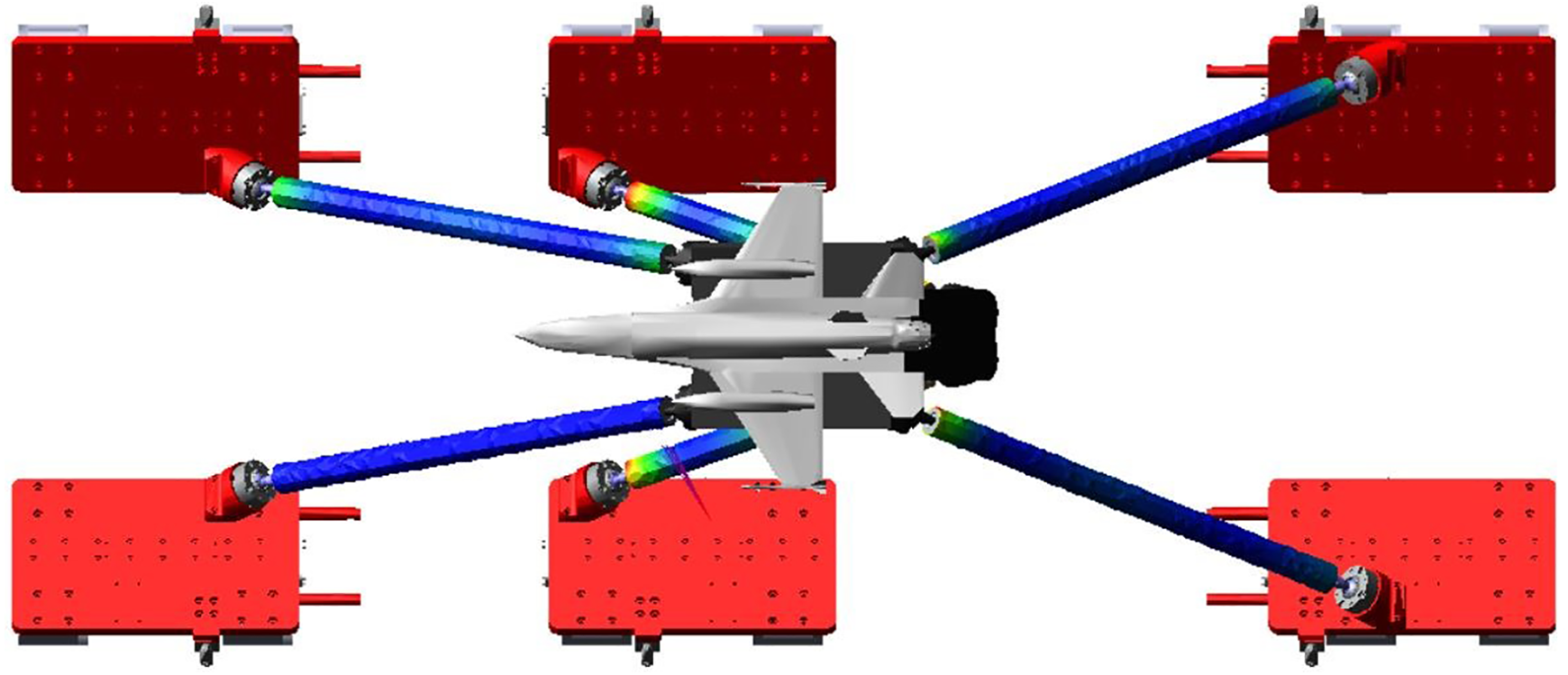
Flexible simulation model of the considered manipulator.

Figure 11.

Curves of displacement.

Figure 12.

Curves of driving force.

In this section, analysis of rigid-body dynamics in conducted by Matlab and Adams, and the correctness of the numerical model is validated by the simulation results. A simplified approach is proposed for flexible dynamics analysis, which is also proved to be effective by simulations within Adams.

Conclusions

In this work, a 6-DOF parallel manipulator with six PSU kinematic chains is presented to support the aircraft models for wind tunnel tests. The mobility analysis is conducted by screw theory, and the inverse position problem is addressed by the principle of homogeneous coordinate transformation. Moreover, the first-order influence coefficient method is utilized for the velocity analysis. On the other hand, Lagrange formulation is employed to establish the rigid-body dynamics model, and a simplified method is proposed for flexible dynamics analysis.

A contribution of this work is taking screw theory and first-order influence coefficient method into consideration for kinematics analysis. With the aid of screw theory, the property of mobility is revealed. The first-order influence coefficient method just relates to the position and orientation of the manipulator, which makes it simple to conduct the velocity analysis. Another contribution is the proposed method for flexible dynamics analysis. The procedure of calculation and simulation will be very complicated if the whole manipulator is taken into flexible processing. Simulation results validate the efficiency of the newly proposed method, which can provide a reference for the flexible dynamics analysis of similar parallel manipulators.

In this work, we mainly address the basic kinetics and dynamics problems, and the proposed method is only proved by software simulation. Needless to say, the test of the physical prototype should also be taken into consideration to validate the efficiency of the proposed method. Moreover, prototype development and experiment will be the topics of future work.

Footnotes

Declaration of conflicting interests

The author(s) declared no potential conflicts of interest with respect to the research, authorship, and/or publication of this article.

Funding

The author(s) disclosed receipt of the following financial support for the research, authorship, and/or publication of this article: This work was financially supported by the Key Project of Natural Science Research in Universities of Anhui Province (KJ2021A1526, KJ2020A1114, KJ2019ZD75), the Key research and development project of Wuhu Science and Technology Bureau (2021yf52), Advanced Manufacturing Technology Application Research Institute Project (2021kjtd02), the Project of 3D printing technology to promote and practice the teaching mode innovation of industrial design major in higher vocational colleges (2020jyxm0305), Practice and research on the construction and operation mechanism of the integration of production and education training base from the perspective of multiple synergies—Taking the cooperation model of Anhui Bowu Modern Industrial Park as an example (2021jyxm0242), the Science and Technology Research Program of Chongqing Municipal Education Commission (KJQN202101114, KJCX2020044, KJQN202201115, HZ2021011).

ORCID iD

Na Wang

References

Chen

Lin

Wei

, et al. Tension vector and structure matrix associated force sensitivity of a 6-DOF cable-driven parallel robot. Proceed Inst Mech Eng, Pt C: J Mech Eng Sci 2022; 236(1): 100–114.

Wang

, et al. Kinematic design and analysis of a 6-DOF spatial five-bar linkage. Mech Mach Theory 2021; 158: 104227.

Staicu

Shao

Zhang

, et al. Kinematic analysis of the X4 translational–rotational parallel robot. Int J Adv Robot Syst 2018; 15(5): 1729881418803849.

Antonov

Fomin

Glazunov

, et al. Inverse and forward kinematics and workspace analysis of a novel 5-DOF (3T2 R) parallel–serial (hybrid) manipulator. Int J Adv Robot Syst 2021; 18(2): 1729881421992963.

Araujo-Gómez

Díaz-Rodríguez

Mata

, et al. Kinematic analysis and dimensional optimization of a 2R2T parallel manipulator. J Brazil Soc Mech Sci Eng 2019; 41(10): 1–9.

Zarkandi

. Kinematic analysis and workspace optimization of a novel 4RPSP + PS parallel manipulator. Mech Bas Design Struct Mach 2021; 49(1): 131–153.

Fomin

Antonov

Glazunov

, et al. Inverse and forward kinematic analysis of a 6-DOF parallel manipulator utilizing a circular guide. Robotics 2021; 10(1): 31.

Zhang

, et al. Mobility, kinematic analysis, and dimensional optimization of new three-degrees-of-freedom parallel manipulator with actuation redundancy. J Mech Robot 2017; 9(4): 041008.

Nayak

Caro

Wenger

. Kinematic analysis of the 3-RPS-3-SPR series–parallel manipulator. Robotica 2019; 37(7): 1240–1266.

10.

Fang

Tang

Zhang

. Kinematic analysis and comparison of a 2R1T redundantly actuated parallel manipulator and its non-redundantly actuated forms. Mech Mach Theory 2019; 142: 103587.

11.

Leal-Naranjo

J-A

Wang

Paredes-Rojas

J-C

, et al. Design and kinematic analysis of a new 3-DOF spherical parallel manipulator for a prosthetic wrist. J Brazil Soc Mech Sci Eng 2020; 42(1): 1–12.

12.

Chen

Wang

, et al. Design and kinematic analysis of a spherical parallel manipulator using concurrent planar parallelogram linkages. Proceed Inst Mech Eng Pt C: J Mech Eng Sci 2019; 233(7): 2491–2501.

13.

Thomas

M J

Joy

Sudheer

. Kinematic and dynamic analysis of a 3-PRUS spatial parallel manipulator. Chinese J Mech Eng 2020; 33(1): 1–17.

14.

Pedrammehr

Nahavandi

Abdi

. Closed-form dynamics of a hexarot parallel manipulator by means of the principle of virtual work. Acta Mechanica Sinica 2018; 34(5): 883–895.

15.

Chen

, et al. Dynamic modeling and performance analysis of the 3-PRRU 1T2R parallel manipulator without parasitic motion. Nonl Dynam 2017; 90(1): 339–353.

16.

Gallardo-Alvarado

Rodriguez-Castro

Delossantos-Lara

. Kinematics and dynamics of a 4-PRUR Schönflies parallel manipulator by means of screw theory and the principle of virtual work. Mech Mach Theory 2018; 122: 347–360.

17.

Liang

Song

Sun

, et al. Dynamic modeling and hierarchical compound control of a novel 2-DOF flexible parallel manipulator with multiple actuation modes. Mech Syst Sig Process 2018; 103: 413–439.

18.

Korayem

Dehkordi

. Dynamic modeling of flexible cooperative mobile manipulator with revolute-prismatic joints for the purpose of moving common object with closed kinematic chain using the recursive Gibbsâ€”Appell formulation. Mech Mach Theory 2019; 137: 254–279.

19.

Zheng

. A novel parallel recursive dynamics modeling method for robot with flexible bar-groups. Appl Mathemat Model 2020; 77: 267–288.

20.

Wang

. Dynamics investigation of spatial parallel mechanism considering rod flexibility and spherical joint clearance. Mech Mach Theory 2019; 137: 83–107.

21.

Gallardo-Alvarado

Garcia-Murillo

Alcaraz-Caracheo

, et al. Forward kinematics and singularity analyses of an uncoupled parallel manipulator by algebraic screw theory. IEEE Access 2021; 10: 4513–4522.

22.

Xie

Kepler

, et al. A parametric model of 3-PPR planar parallel manipulators for optimum shape design of platforms. Mech Mach Theory 2017; 118: 139–153.

23.

Liu

Yang

, et al. Design and analysis of a novel 12-DOF self-balancing lower extremity exoskeleton for walking assistance. Mech Mach Theory 2022; 167: 104519.

24.

Liu

. Synthesis of asymmetric parallel mechanism with multiple 3-DOF motion modes. Adv Mech Eng 2022; 14(2): 16878140221075309.

Kinematics and dynamics analysis of a six-degree of freedom parallel manipulator

Abstract

Keywords

Introduction

A 6-DOF parallel manipulator

Manipulator description

Mobility analysis

Inverse position analysis

Velocity analysis

Velocities of the sliders

Velocities of struts

Inverse dynamics model

Kinetic energy

Potential energy

Dynamics model

Simulation

Simulation of the rigid-body dynamics

Simulation of the simplified flexible dynamics

Conclusions

Footnotes

Declaration of conflicting interests

Funding

ORCID iD

References