Sage Journals: Discover world-class research

Abstract

To improve the finding path accuracy of the ant colony algorithm and reduce the number of turns, a jump point search improved ant colony optimization hybrid algorithm has been proposed in this article. Firstly, the initial pheromone concentration distribution gets from the jump points has been introduced to guide the algorithm in finding the way, thus accelerating the early iteration speed. The turning cost factor in the heuristic function has been designed to improve the smoothness of the path. Finally, the adaptive reward and punishment factor, and the Max–Min ant system have been introduced to improve the iterative speed and global search ability of the algorithm. Simulation through three maps of different scales is carried out. Furthermore, the results prove that the jump point search improved ant colony optimization hybrid algorithm performs effectively in finding path accuracy and reducing the number of turns.

Keywords

Mobile robot path planning jump point search algorithm ant colony optimization algorithm turn cost factor

Introduction

As an important part of kinematics, path planning is widely used in unmanned aerial vehicle (UAV),¹ robot,² and automated guided vehicle (AGV).³ Path planning for mobile robots refers to planning a path from starting node to the target node. It requires the path to be safe, collision-free, and the comprehensive indicators such as distance, time, and energy consumption are optimal.⁴

Currently, a lot of scholars have done much research on the path planning problem and proposed a wide variety of algorithms, such as A* algorithm,⁵ ant colony optimization⁶ (ACO) algorithm, genetic algorithm⁷ (GA), particle swarm optimization algorithm,⁸ artificial potential field method⁹ (APF), fireworks algorithm¹⁰ (FA), and so on.

ACO algorithm is a heuristic algorithm first proposed by Dorigo and Maniezzo in the 1990s,¹¹ and it imitates the foraging behavior of ant colonies in nature. It’s widely used in path planning because of its strong robustness, positive feedback enhancement of optimal path, and ease of combination with other algorithms. However, there are some problems, such as slow convergence speed, easy trap into a locally optimal solution. To address these problems, plenty of scholars have conducted in-depth research. Sun et al.¹² greatly improved the survival number of ants in the algorithm and accelerated the convergence rate of the algorithm by adopting different strategies for deadlock problems in the algorithm. Zhang et al.¹³ improved the ability of search space by using information entropy to describe the ant colony and construct a nonuniform distribution of pheromone concentration and renewal mechanism. Zhang et al.¹⁴ accelerated the convergence rate of the algorithm and operating efficiency by dividing the ant colony into guide layer ant colony and common layer ant colony to search path. Khaled and Farid¹⁵ accelerated the algorithm’s convergence rate and increased the search scope by using a new pheromone updating rule and dynamic evaporation rate. Luo et al.¹⁶ made the initial pheromone uneven distribution to avoid the early blind search of the algorithm, speed up the convergence of the algorithm, and used the dynamic punishment method to reduce the number of ants trapped in a deadlock. Meng et al.¹⁷ proposed a multi-ant colony cooperative optimization algorithm based on a cooperative game mechanism to accelerate the convergence speed of the algorithm. Tao et al.¹⁸ used fuzzy control to change the value of the pheromone heuristic factor and expectation heuristic factor and adjusted the evaporation rate in stages, which ensured the global search ability of the algorithm.

With the development of algorithms, the ACO algorithm gradually began to combine with other algorithms to achieve the purpose of an optimization algorithm. Ma et al.¹⁹ used the improved FA to generate the initial pheromone concentration values to distribute them on the map and then search for a globally optimal path through the ACO algorithm. This algorithm can find the optimal path in the case of fewer iterations. Dai et al.²⁰ accelerated the algorithm’s convergence rate and improved the path’s smoothness by adding evaluation functional and bending inhibitors of the A* algorithm. Zhu et al.²¹ improved the fitness function of the ant colony algorithm by using the APF algorithm, and the adjustment of negative feedback and self-fitness function was taken into account at the same time. Therefore, this method can greatly accelerate the convergence rate of the algorithm. Yu²² gave the concept of an ant colony particle and fused the particle swarm algorithm with the ACO algorithm to improve the convergence speed of the algorithm. Lei et al.²³ used the GA to generate the initial path and took the better path as the reference information of the ant colony algorithm pheromone initialization to reduce the blindness of the initial search of the ant colony algorithm. Then, the ant colony algorithm was used to further optimize the initial path and accelerate the convergence speed of the algorithm. Saenphon et al.²⁴ used the fast reverse gradient method to obtain the possible optimal solution and then used the ACO algorithm to further improve the quality of the solution. Li et al.²⁵ proposed optimization ants and reconnaissance ants combined with the artificial bee colony algorithm and assigned different pheromone updating weights, respectively. The convergence speed of the algorithm is improved to avoid the algorithm falling into local optimum and ensure the diversity of solutions.

Based on the above literature research, the JPIACO algorithm is proposed in this article. The main contributions of this work are as follows:

The initial pheromone concentration distribution obtained from the jump point search (JPS) algorithm is designed to accelerate the early iteration speed.

A new heuristic function is designed to improve the smoothness of the path.

A new adaptive reward and punishment factor is designed to improve the iterative speed.

The Max–Min ant system has been introduced to improve the global search ability.

The framework of the article is as follows. The second section describes the map establishment method. The third section mainly describes the JPS algorithm. The fourth section mainly describes the JPIACO algorithm. The fifth section describes the experiments and results. The sixth section summarizes the thesis.

Environment model

In the path planning of mobile robots, we should establish a 2D model of the robot movement environment firstly, and the modeling methods include the free space method, grid method, topology method, and so on. Simple, effective, easy to implement, and can clearly express obstacles are considered, the grid method to model is used in this article. An example of the grid map is shown in Figure 1.

Figure 1.

Schematic diagram of grid map encoding.

In the grid map, white grids are free spaces that robots can move and black grids are obstacle spaces that robots can’t move. To save the path and pheromone concentration easily, numbered the grid map by the way from left to right and top to bottom. As the numbers show in Figure 1, from left to right and top to bottom, the map numbers the grid starting at 1 until it is added to the 100th grid in the lower right corner.

The relationship between its coordinates and the number n of the grid is shown in equation (1)

{\begin{array}{l} X_{n} = {\begin{cases} mod (n, M M) - 0.5, X_{n} \neq - 0.5 \\ M M - 0.5, X_{n} = - 0.5 \end{cases} \\ Y_{n} = ceil (\frac{n}{M M}) - 0.5 \end{array}

where MM is the number of grids per row, mod represents the operation of complementation, and ceil(n/MM) represents the integer operation not less than n/MM.

Initial path planning based on the JPS algorithm

The JPS algorithm is the optimization of the A* algorithm. In the traditional A* algorithm, path analysis of each step needs to calculate the value of the eight direction nodes around, it generates a lot of unnecessary calculation steps which reduces the efficiency of the algorithm. While the JPS algorithm discards unnecessary nodes, leaving only representative nodes in the path search (these nodes are called jump points), it greatly improves the running efficiency of the algorithm.

Jump point screening

In the grid map, use each grid as a node, define eight grids adjacent to the current node grid as “around the current node,” the current node position is the parent node P(x) and the next node to move is x. There are two cases in jump point screening, one is when there are no obstacles around the current node, and the other is when there are obstacles around the current node.²

Case 1: There are no obstacles around the current node

In Figure 2(a), when searching from point P(x) to the right, the path generated by P(x) passing through node x to the next node n (such as 4→5→6) in this direction is the shortest compared with P(x) to the next node n without through node x (such as 4→ $\dots$ →6 without through node 5), so the gray nodes(1,2,3,4,7,8) are the unnecessary node and does not need to calculate the path generation value, define these gray nodes as invalid nodes. Therefore, when there are no obstacles around the node, the screening conditions in the horizontal and vertical directions are as follows

L (P (x), \dots, n / x) \geq L (P (x), x, n)

where L(·) represents path length, <P(x),…, n>/x is a path from P(x) to n without going through x; <P(x), x, n> is the path P(x)→x→n and n is the movable node around node x.

Figure 2.

Pathfinding process of obstacle-free nodes around the node x. (a) Linear movement and (b) diagonal movement.

In Figure 2(b), when searching from point P(x) to the diagonal direction, similarly, gray nodes (1, 2, 3, 4, 7) are invalid nodes and do not need to calculate the path generation value, define the white nodes around node x as natural neighbors. Therefore, when there are no obstacles around the node, the screening condition in the diagonal direction is as follows

L (P (x), \dots, n / x) > L (P (x), x, n)

Case 2: There are obstacles around the current node

As shown in Figure 3, there is an obstacle node (2 in Figure 3(a) and 4 in Figure 3(b)) around node x, the method of searching nodes with no obstacles cannot be used for screening, and a new screening rule must be adopted. In this time, the distance from P(x) to the next node n through node x (such as 4→5→3 in Figure 3(a)) is the shortest path compared with P(x) to the next node n without through node x (such as 4→ $\dots$ →3 without through node 5 in Figure 3(a)), and node n is not a natural neighbor of node x, call the node n is the mandatory neighbor of node x. Therefore, MN in Figure 3(a) and 3(b) are mandatory neighbor points. The screening conditions for mandatory neighbor points are as follows:

n is not the natural neighbor of node x

$L (P (x), \dots, n / x) > L (P (x), x, n)$

Figure 3.

Pathfinding process of obstacle nodes around the node x. (a) Linear movement and (b) diagonal movement.

Figure 4.

JPS algorithm pathfinding process. JPS: jump point search.

In summary, a jump point is defined as meeting at least one of the following three conditions:

Node x is the start or end point.

Node x has at least one mandatory neighbor point.

When node x moves in the diagonal direction, there are points satisfying conditions (1) and (2) in its horizontal and vertical directions.

Path generation

After jump point screening, the obtained jump points are added to the Openlist table of the A* algorithm for evaluation, and the evaluation function is shown in equation (4)

f (n) = h (n) + g (n)

where f(n) is the evaluation function, h(n) is the path cost from the current node to the target node, and g(n) is the path cost from the start node to the current node. This algorithm uses the Euclidean distance between two points as the path of the cost.

Select the target node with the lowest cost value and add it to the Closelist table of the A* algorithm, then connect the nodes in the Closelist table and we can get the path.

The A* algorithm can only select eight adjacent directions for calculation in the next node selection, but the JPS algorithm can choose from jump points, and achieve movement across multiple node distances, which greatly improved the operating efficiency.

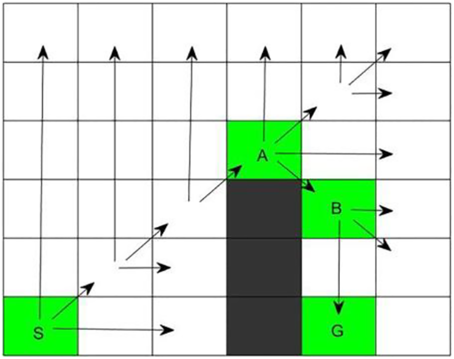
As shown in Figure 4, S is the start point and G is the target point. Firstly, record start point S as the jump point according to the jump point rule, search in the horizontal and vertical directions, and the search stops when encountering a map boundary or obstacle, after searching in horizontal and vertical directions, move a grid diagonally to continue the horizontal and vertical search. Repeat the above operation, when moving to point A find mandatory neighbor point B, and record the start point A and B as the jump point according to the jump point rule. Point B search down and find the goal point G, record the goal point G as a jump point, and stop the search. Finally, we can get the path through the relationship between the parent node and the child node.

JPIACO algorithm

ACO algorithm

ACO algorithm is to imitate the foraging behavior of ant colonies in nature. It obtains the optimal path by continuously updating the pheromone between colony and environment. The shorter path that the ant walks, the more concentration of pheromones left, the ant has a higher probability to choose the path, so there will be more and more pheromones on the path, thus forming an optimal path positive feedback strengthening mechanism.

In the ACO algorithm, roulette is generally used to select the next node, as shown in equation (5)

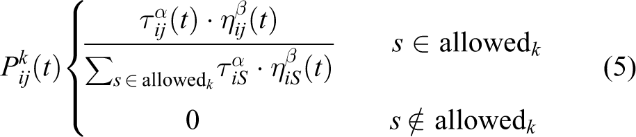
P_{i j}^{k} (t) \{\begin{matrix} \begin{matrix} \frac{τ_{i j}^{α} (t) \cdot η_{i j}^{β} (t)}{\sum_{s \in {allowed}_{k}} τ_{i S}^{α} \cdot η_{i S}^{β} (t)} & s \in {allowed}_{k} \end{matrix} \\ \begin{matrix} 0 s \notin {allowed}_{k} \end{matrix} \end{matrix}

where τ_ij (t) is the pheromone concentration between node i and node j, η_ij = 1/d_ij is the heuristic function and d_ij is the Euclidean distance; j is the next mobile node and s is an unprocessed node; α and β are two constants, respectively, represent the importance of pheromone concentration and heuristic function; allowed _k is a collection of nodes that have not yet passed.

When the ACO algorithm completes a loop search, the pheromone on the path is updated globally, the calculation formula is shown in equations (6) and (7)

\{\begin{array}{l} τ_{i j} (t + 1) = (1 - ρ) τ_{i j} (t) + Δ τ_{i j} \\ Δ τ_{i j} = \sum_{k = 1}^{m} Δ τ_{i j}^{k} \end{array}

Δ τ_{i j}^{k} = \{\begin{array}{l} \begin{matrix} \frac{Q}{L_{k}} & find the path \end{matrix} \\ \begin{matrix} 0 & others \end{matrix} \end{array}

where ρ is the pheromone evaporation coefficient between 0 and 1, m is the number of ants, Q is a constant greater than 0, and L_k is the length of the path found by the ant k.

Improvement of ACO algorithm

For the shortcomings of the ACO algorithm such as slow iteration speed and unsmooth path, modify the heuristic function of the ACO algorithm, introduce the reward and punishment factor from the Wolf pack colony algorithm, and limit the maximum and minimum ant pheromone concentration.

Design of heuristic function

The heuristic function of the ACO algorithm is reciprocal to the Euclidean distance from the current node to the target node, but in fact, the mobile robot will generate extra time when turning in motion, so the path will be selected with fewer turns when the path length is equal. Based on this, the cost of turns is added to the heuristic function to make the generate path smoother, heuristic function is shown in equations (8) and (9)

η_{i j} (t) = \frac{1}{d_{i j} + c_{i j}}

c_{i j} = ω \cdot ψ \cdot θ

where ω(0<ω<1) is the weight of turning cost, ψ is the factor converted to grid length, and θ is the angle between the forward and backward motion directions of the current node.

Improvement of initial pheromone

The pheromone concentration of each node in the early stage of the ACO algorithm is the same, which leads to the problem of blind path search, poor convergence, and long search time. To address this problem, this algorithm first finds a series of jump points by the JPS algorithm, and these jump points produce a guiding effect in the early stage, which speeds up the previous iteration, the initial concentration value is shown in equation (10)

Gau = \frac{Q}{L_{jps}} \cdot \frac{D_{sum}}{D_{jps}}

where Gau is the initial pheromone concentration value at each jump point, L _jps is the path length found by the JPS algorithm, D _sum is the total number of points passed by the path, and D _jps is the number of jump points.

Improvement in pheromone update

For the shortcomings of the ACO algorithm in convergence speed slow, introduce reward and punishment factors in the Wolf pack algorithm.²⁶ After each iteration, pheromone reward for the optimal path and penalty for the worst path. Furthermore, aim at the difference between pathfinding in early and later stages of iteration, conduct dynamic adjustment of pheromone concentration by increasing the reward and punishment factors in early iteration and decreasing the factors in the late iteration, because it’s necessary to quickly find a relative path in the early stage and increase the search range in the later stage. The formula is defined as follows

\{\begin{cases} τ_{i j} (t + 1) = (1 - ρ) τ_{i j} (t) + Δ τ_{i j} + pau \\ Δ τ_{i j}^{k} = \sum_{k = 1}^{m} Δ τ_{i j}^{k} \\ Δ τ_{i j}^{k} = {\begin{matrix} \frac{Q}{L_{k} + C_{k}} & find the path \\ 0 & others \end{matrix} \\ pau
 
= {\begin{cases} \frac{(1 - \frac{n}{N}) . Q}{L_{k} + C_{k}}, optimal
 
path
 
of
 
this
 
iteration \\ \frac{(- 1 + \frac{n}{N}) . Q}{L_{k} + C_{k}}, worst
 
path
 
of
 
this
 
iteration \\ 0,
 
others \end{cases} \end{cases}

where Pau is the reward and punishment factor, C_k is the total turn cost of ant k, n and N are, respectively, the current number and the total number of iterations, other parameters are consistent with the ACO algorithm.

In the ACO algorithm, the pheromone concentration on one path is much higher than on other paths after multiple iterations, which may trap into the local optimum and lose the global optimum solution. To avoid it, introduce the Max and Min system to limit it²⁷, the formula is shown in equation (12)

Tau = \{\begin{array}{l} {Tau}_{min},                  , Tau \leq {Tau}_{min} \\ {Tau,       ,   Tau}_{min} \leq Tau \leq {Tau}_{max} \\ {Tau}_{max},, {Tau}_{max} \leq Tau \end{array}

where Tau is the total pheromone concentration at any point on the map.

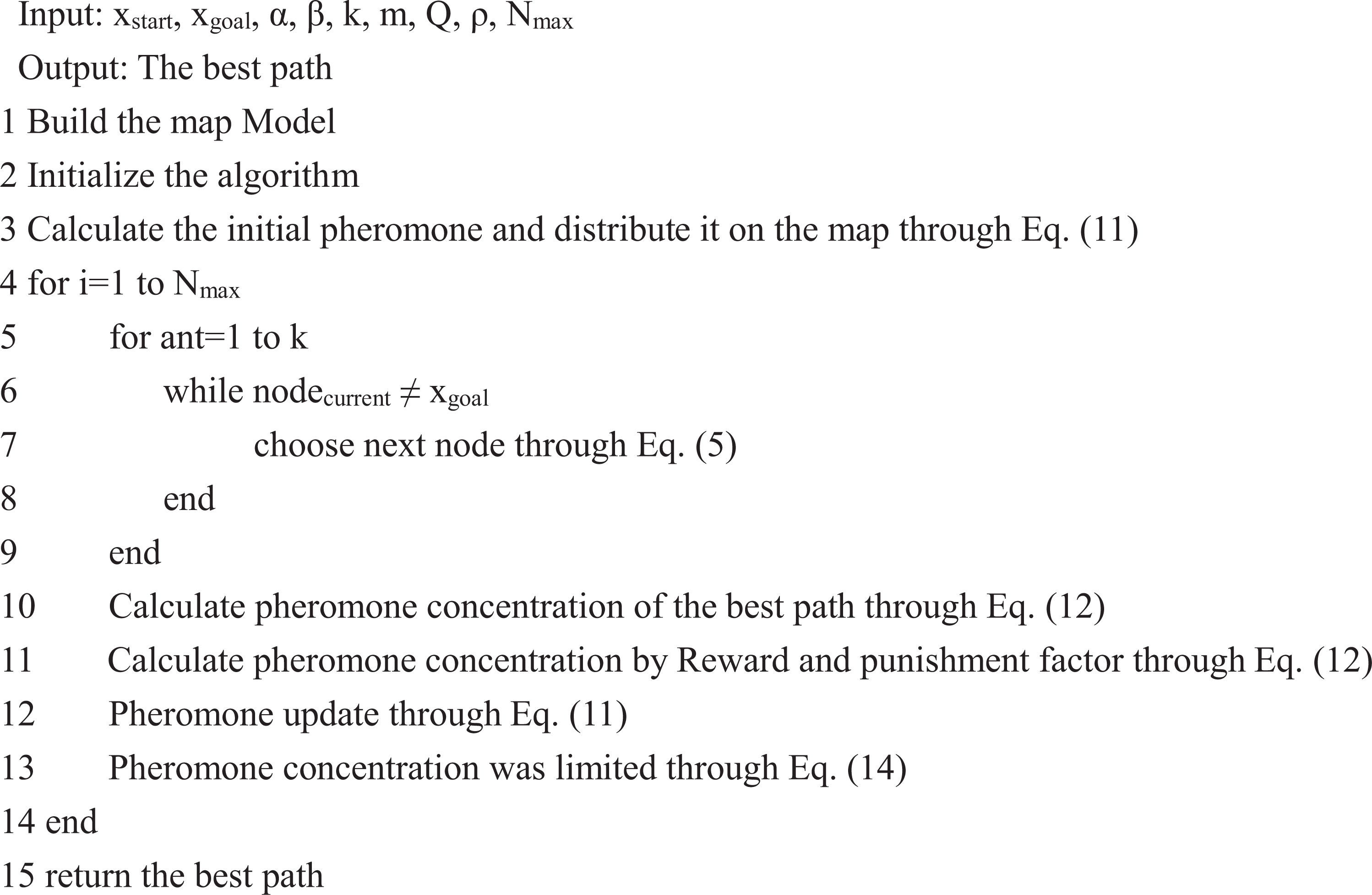
As shown in Algorithm 1, this is the pseudo-code of the JPIACO algorithm.

Algorithm 1.

JPIACO algorithm.

Simulation

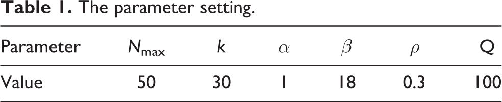
So as to verify the effectiveness of the proposed algorithm in path planning, compare it with the ACO algorithm through path length, iteration times, and number of turns. Experiments were run on an Intel i7-4720HQ cpu with 8G of RAM, and the programming language is MATLAB(R2018b). The ACO algorithm parameters are set according to the literature,^10,12,28 set according to the original parameters, and the parameters set in this article are shown in Table 1.

Table 1.

The parameter setting.

Parameter	N _max	k	α	$β$	$ρ$	Q
Value	50	30	1	18	0.3	100

As shown in Figure 5, use map 1 (15*15), map 2 (30*30), and map 3 (50*50) in the literature⁷ as the environment for simulation experiments.

Figure 5.

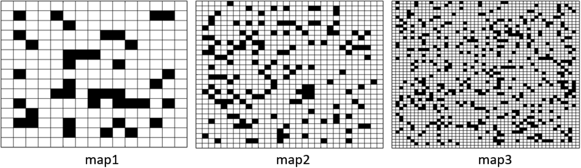
Three kinds of maps.

Figures 6(a), 7(a) and 8(a) are the optimal paths of the ACO algorithm under three maps; Figures 6(b), 7(b), and 8(b) are the optimal paths of JPIACO algorithm; Figures 6(c), 7(c), and 8(c) are the optimal path length iteration curve comparison of two algorithms.

Figure 6.

Comparison of map 1. (a) ACO optimal path in map 1; (b) JPIACO optimal path in map 1; (c) iterations comparison of ACO and JPIACO in map 1.

Figure 7.

Comparison of map 2. (a) ACO optimal path in map 2; (b) JPIACO optimal path in map 2; (c) iterations comparison of ACO and JPIACO in map 2.

Figure 8.

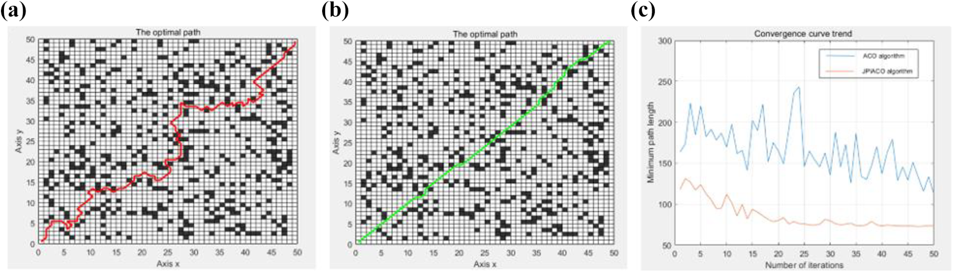
Comparison of map 3. (a) ACO optimal path in map 3; (b) JPIACO optimal path in map 3; (c) iterations comparison of ACO and JPIACO in map 3.

As seen from Figures 6 to 8, the ACO algorithm finds the relatively optimal shortest path in the small environmental scale map, but with the increase of environmental scale, there are a lot of twists and turns in the path. However, the JPIACO algorithm can always find the relatively better shortest path. Moreover, the ACO algorithm finds the relative shortest path after 13 times in the environment of map 1, with the increase of the environment scale, the iterative process has not stabilized and the path is not optimal as we can see. But the JPIACO algorithm can find the relative optimal path in few times, it stabilized after 2 iterations in map 1, stabilized after 6 iterations in map 2, and stabilized after 22 iterations in map 3. It further confirms the effectiveness of the JPIACO algorithm.

To verify the performance advantages of the JPIACO algorithm in path planning, compare it with the ACO algorithm and algorithm of literature^10,12 to obtain the number of turns, minimum iteration, and optimal path length in three maps environments, as shown in Table 2.

Table 2.

Simulation experiment results.

Algorithm	Map 1			Map 2			Map 3
Algorithm	Optimal path length	Number of turns	Minimum iteration	Optimal path length	Number of turns	Minimum iteration	Optimal path length	Number of turns	Minimum iteration
ACO	20.97	5	13	44.18	9	50	112.4	66	50
Literature¹⁰	20.97	6	6	41.59	3	12	77.15	22	15
Literature¹²	20.97	7	10	42.51	12	18	75.12	23	22
JPIACO	20.97	4	1	41.59	2	6	71.64	15	22

As seen from Table 2, with the increase in the complexity of the environment, the ACO algorithm finds a larger and larger gap in the length of the path compared to the JPIACO algorithm, from a difference of 4 in map 2 to a difference of 48.14 in map 3, the number of turns and minimum iteration are the largest among the four algorithms in three maps expect in map 1. The algorithm proposed in the literature¹⁰ can find the optimal solution in a few iterations, with the increase of environmental complexity, the optimal path length found in the environment of map 3 is 77.15, which is still insufficient compared with 71.64 found by the JPIACO algorithm, the number of turns is deficiency compare with this article, but for the minimum number of iterations, literature¹⁰ found the minimum iteration in map 3. The algorithm proposed in the literature¹² can deal with deadlock better, but the path found in map 2 and map 3 is inferior to the JPIACO algorithm, the number of turns and minimum iteration among the four algorithms are inferior to this article. In terms of path accuracy and the number of turns, the algorithms proposed in this article find the best path and the least turns among the four algorithms, for the minimum number of iterations, this article is optimal between map 1 and map 2, and second only to the literature¹⁰ in map 3. What’s more, in terms of turning angle, the algorithm in this article is 45° turning angle, compared with 90° turning angle and 135° turning angle existing in other algorithms, the cost of turning is smaller and more in line with the actual path planning application, which has a great practical value.

Conclusion

This article presents the JPIACO algorithm. Aiming at the problems of the ACO algorithm, such as slow early convergence speed and an excessive number of turning points, the JPS algorithm is added to obtain jump points by guiding a pathfinding function to distribute initial pheromone concentration values in the map. The turn cost factor, additional reward and punishment factors, and Max–Min ant system are added, and these improve the shortcomings of slow convergence speed and a lot of turns of the ACO algorithm. JPIACO algorithm is simulated under three kinds of maps and compared with the algorithm in literature,^10,12 and the results show that the JPIACO algorithm has an improved effect, which can quickly find an effective path with high precision, few turning points, and small turning angles. Moreover, it is still effective in complex environments. The simulation results of different map sizes show that the JPIACO algorithm is generally adaptable to map scale and obstacle distribution structure.

Although JPIACO is a promising algorithm, the kinematic constraints must be considered if applied to robots. In addition, the performance of the algorithm in the dynamic environment should also be verified, and that’s what we’re going to do in the future.

Footnotes

Declaration of conflicting interests

The author(s) declared no potential conflicts of interest with respect to the research, authorship, and/or publication of this article.

Funding

The author(s) disclosed receipt of the following financial support for the research, authorship, and/or publication of this article: This work was supported by National Key Research and Development Program of China (Grant No. SQ2020YFF0423771) and Zhejiang Science and Technology planning project (Grant No. 2020C01053).

ORCID iD

Tao Chen

References

Zhao

Zheng

Liu

. Survey on computational-intelligence-based UAV path planning. Knowledge-Based Syst 2018; 158: 54–64.

Cao

Zhou

. An efficient RRT-based framework for planning short and smooth wheeled robot motion under kinodynamic constraints. IEEE Trans Indust Electr 2020; 68: 99.

Wang

. An improved timed elastic band (TEB) algorithm of autonomous ground vehicle (AGV) in complex environment. Sensors 2021; 21: 8312.

Zhu

Yan

. Survey on the technology of mobile robot path planning. Contr Decis 2010; 25(7): 961–967.

Zhao

Wang

Huang

, et al. Mobile robot path planning based on an improved A* algorithm. Robot 2018; 40(6): 903–910.

Yuan

Wei

Shen

, et al. Research on path planning based on new fusion algorithm for an autonomous vehicle. Int J Adv Robot Syst 2020; 17(3): 172988142091123.

Kumar

Parhi

. Intelligent navigation of humanoids in cluttered environments using regression analysis and genetic algorithm. Arabian J Sci Eng 2018; 43(12): 7655–7678.

Petrović

Vuković

Mitić

, et al. Integration of process planning and scheduling using chaotic particle swarm optimization algorithm. Exp Syst Appl 2016; 64: 569–588.

Wang

Gao

, et al. Obstacle avoidance path planning design for autonomous driving vehicles based on an improved artificial potential field algorithm. Energies 2019; 12(12): 2342.

10.

Zhang

Zhao

, et al. Obstacle avoidance path planning of intelligent mobile-based on improved fireworks-ant colony hybrid algorithm. Contr Decis 2019; 34(2): 335–343.

11.

Dorigo

Maniezzo

Colorni

. Ant system: optimization by a colony of cooperating agents. IEEE Trans Syst Man Cybern Pt B Cybern 1996; 26(1): 29–41.

12.

Sun

, et al. Path planning for unmanned surface vehicle based on improved ant colony algorithm. Contr Decis 2021; 36(4): 847–885.

13.

Zhang

. An adaptive improved ant colony system based on population information entropy for path planning of mobile robot. IEEE Access 2021; 9: 99.

14.

Zhang

Yuan

, et al. Mobile robot path planning using improved double-layer ant colony algorithm. Contr Decis 2022; 37(02): 303–313.

15.

Khaled

Farid

. Mobile robot path planning using an improved ant colony optimization. Int J Adv Robot Syst 2018; 15(3): 172988141877467.

16.

Luo

Wang

Zheng

, et al. Research on path planning of mobile robot based on improved ant colony algorithm. Neural Comput Applic 2020; 32: 1555–1566.

17.

Meng

You

Liu

. Multi-colony collaborative ant optimization algorithm based on cooperative game mechanism. IEEE Access 2020; 8: 99.

18.

Tao

Gao

Ren

, et al. A mobile service robot global path planning method based on ant colony optimization and fuzzy control. Appl Sci 2021; 11(8): 3605.

19.

Mao

Wang

, et al. Obstacle avoidance path planning of unmanned submarine vehicle in ocean current environment based on improved firework-ant colony algorithm. Comput Electr Eng 2020; 87: 106773.

20.

Dai

Long

Zhang

, et al. Mobile robot path planning based on ant colony algorithm with A* heuristic method. Front Neurorobot 2019; 13: 15.

21.

Zhu

Zhang

, et al. Path planning of lunar robot based on dynamic adaptive ant colony algorithm and obstacle avoidance. Int J Adv Robot Syst 2020; 17(3): 4149–4171.

22.

. A solution of TSP based on the ant colony algorithm improved by particle swarm optimization. Discrete Contin Dynam Syst S 2018; 12(4): 979–987.

23.

Lei

Luo

, et al. Trajectory planning of an autonomous mobile robot by evolving ant colony system. Int J Robot Auto 2017; 32(4): 1500–1515.

24.

Saenphon

Phimoltares

Lursinsap

. Combining new fast opposite gradient search with ant colony optimization for solving traveling salesman problem. Eng Appl Artif Intell 2014; 35: 324–334.

25.

You

Liu

. Dynamic hierarchical dual-morphic ant colony algorithm based on artificial bee colony algorithm. Comput Eng Appl 2020; 56(12): 37–46.

26.

Zhang

. A new swarm intelligence algorithm—wolf pack algorithm. Syst Eng Electr Technol 2013; 35(11): 2430–2438.

27.

Stützle

Hoos

. MAX–MIN ant system. Fut Gen Comput Syst 2000; 16: 889–914.

28.

Shi

Chen

, et al. Research on method of global path planning for mobile robot based on the ant-colony algorithm. Trans Chinese Soc Agricul Mach 2014; 45(6): 53–57.

A jump point search improved ant colony hybrid optimization algorithm for path planning of mobile robot

Abstract

Keywords

Introduction

Environment model

Initial path planning based on the JPS algorithm

Jump point screening

Path generation

JPIACO algorithm

ACO algorithm

Improvement of ACO algorithm

Design of heuristic function

Improvement of initial pheromone

Improvement in pheromone update

Simulation

Conclusion

Footnotes

Declaration of conflicting interests

Funding

ORCID iD

References