Sage Journals: Discover world-class research

Abstract

This paper introduces CLAM, a hybrid deep learning framework that integrates CNNs, LSTMs, and Attention Mechanism (AM) for straightforward multi-step stock trend forecasting. By leveraging CNNs for spatial feature extraction, LSTMs for capturing temporal dependencies, and AM for dynamically focusing on relevant data, CLAM significantly outperforms traditional models in predictive accuracy. Evaluated on diverse stock datasets from different industries, CLAM demonstrates an average reduction of over 80% in MAE and RMSE compared to standalone CNN, LSTM, and fused CNN-LSTM. The model’s ability to capture both short-term and long-term trends is particularly advantageous for real-time financial trading, resulting in 75% trend prediction accuracy, with most cases witnessing consecutive accurate forecasts of flash crashes or uptrends, which aids in strategic investment decisions and risk management. Code and data are available at: https://anonymous.4open.science/r/CNN-LSTM-AM-AB13/src/CLAM.ipynb.

Keywords

deep learning stock markets attention mechanism trend prediction

Introduction

Concerning the evolving industrial landscape, technological innovation and financial strategy intersection has become vital (Porter, 1985). Artificial Intelligence (AI) is leading this transformation, with advanced neural network architectures such as Convolutional Neural Networks (CNNs) (LeCun et al., 1998), Recurrent Neural Networks (RNNs) (Mikolov et al., 2010), Long Short-Term Memory Networks (LSTMs) (Hochreiter & Schmidhuber, 1997), and Transformers (Vaswani et al., 2017) driving advancements in healthcare (Esteva et al., 2019) and meteorology (Ham et al., 2019) is well-recognized. Nevertheless, its influence on finance is the most promising (Nguyen et al., 2015) as the digital economy amplified the role of Machine Learning (ML) in financial markets, where predictive modelling is essential for forecasting stock prices (Gu et al., 2018) and informing investment strategies (Henrique & Sobreiro, 2019). Recovering from the pandemic, the need for precise financial predictions has grown strongly (Sharif et al., 2021). Investors increasingly rely on algorithmic modelling to navigate through market complexities, thereby capitalizing on opportunities from quantitative trading of stocks (Hagenau et al., 2013).

Traditional models such as ARIMA (Autoregressive Integrated Moving Average) (Box et al., 2015), SARIMA (Seasonal ARIMA) (De Gooijer & Hyndman, 2011), and Linear Regression (Montgomery et al., 2012) are predicated on the assumption that historical patterns and trends can effectively predict future stock prices. However, the non-linear nature of stock movements often introduces significant biases in these models (Tsay, 2005), which tend to oversimplify complex financial dynamics by assuming fixed data variance and linearity (Cont, 2001). This simplification overlooks critical factors influencing stock prices over time, such as macroeconomic indicators (Fama, 1981), market sentiment (Baker & Wurgler, 2006), and herd behaviour (Bikhchandani et al., 1992). The emergence of Machine Learning (ML) and Deep Learning (DL) models has addressed many of these limitations (Hochreiter & Schmidhuber, 1997). Techniques like Support Vector Machines (SVM) (Vapnik, 1995), Decision Trees (Breiman et al., 1984), and Random Forest Regression (RFR) (Liaw & Wiener, 2002) have advanced the ability to capture non-linear relationships by integrating multiple features and learning from large, complex datasets (Chong et al., 2017). DL, as a subset of ML, has further transformed forecasting with deep neural architectures like CNNs (LeCun et al., 1998), RNNs (Mikolov et al., 2010), and LSTMs (Hochreiter & Schmidhuber, 1997), employing hierarchical end-to-end learning that excels in handling unstructured data and scaling with increasingly large time series datasets (Zhu et al., 2018). Additionally, hybrid models that combine elements of traditional statistical methods with ML and DL techniques are reshaping the forecasting landscape (Zhang et al., 2017). These hybrid approaches, by integrating multiple modalities, enhance feature extraction and provide deeper insights into data irregularities (Wang et al., 2019) for a more robust financial system. Nonetheless, despite their improved accuracy, ML and DL models bring challenges such as overfitting (Hastie et al., 2009), interpretability issues (Lipton, 2018), and the necessity for large datasets.

Building on this concept, this paper introduces the CLAM model to forecast the weekly trend of financial assets. CLAM is a hybrid deep learning architecture that combines stacked layers of CNN, LSTM, and an Attention Mechanism (AM) to address the challenges identified in previous models. Our CLAM leverages CNNs for effective feature extraction, capturing spatial patterns in stock price data. LSTMs are then employed to manage temporal dependencies, effectively handling the sequence of data points over time. The attention mechanism further enhances the model by dynamically focusing on relevant features, allowing the model to prioritize critical information and mitigate the impact of less significant data. This combination of techniques enhances the model’s ability to capture both short-term and long-term dependencies thus strengthening its robustness in handling non-linear relationships within the data. Nonetheless, recognizing the impracticality of forecasting stock price value, CLAM focuses on being a computationally efficient model by only focusing on equity movements, which is well-suited for real-time swing trading within volatile financial markets. CLAM’s strength lies in its straightforward architecture, which follows common financial market operation flow, and real-time applicability, aiming to be a deliberate baseline for stock price predictive modelling tasks. Investors are offered a direct end-to-end solution that ensures reproducibility across common devices.

This paper is organized as follows: Section “Literature Review” reviews financial forecasting literature, emphasizing the limitations of traditional models and advances in hybrid approaches. Section “Methodology” outlines the data processing, metrics, and CLAM architecture. Section “Experiments and Results” describes the experimental setup, model comparisons, and performance results. Section “Discussion” discusses the findings and potential improvements. Finally, Section “Conclusion” summarizes and suggests directions for real-time financial trading applications. CLAM is built on our previous publications (Anh & Ha, 2024a, 2024b; Anh et al., 2024).

Literature Review

Related Work

The stock market represents a complex system influenced by a wide range of often unrelated factors, such as psychological behaviour and economic conditions. Among various forecasting models, the Back Propagation Neural Network (BP-NN) has been shown to outperform others, such as ARIMA and Random Forest Regression (RFR), in predicting the one-year stock prices of Chinese vaccine manufacturers (Chen et al., 2015). This outcome is particularly beneficial for investors within the pharmaceutical sector. Additionally, a combination of Seasonal ARIMA and Extreme Gradient Boosting (SARIMA-XGBoost) has demonstrated impressive accuracy in forecasting the Indian Stock Index (Mahajan & Sinha, 2020), reflecting the potential of hybrid models in achieving high predictive performance. Similarly, the RFR model has been effective in predicting stock prices of companies listed on Indian exchanges, further indicating the utility of ML models in financial forecasting (Bhuriya et al., 2017). These traditional ML approaches have proven effective, but the advent of Deep Learning, a subset of ML, has introduced a new level of precision in model development by autonomously learning hierarchical data representations (LeCun et al., 2015). To advance stock market prediction, Wang et al. (2019) introduced a model that combines the LightGBM algorithm with wavelet packet decomposition (WPD) to filter out data noise before forecasting the Shanghai Composite Index. This hybrid approach successfully predicted the market trend over a 10-day period, surpassing the performance of ARIMA and Support Vector Regression (SVR) (Wang et al., 2019). Furthermore, the integration of CNNs to enhance LSTM networks has led to major improvements in short-term prediction accuracy, showing a 25% increase on the CSI300 index (Qin et al., 2017). A more advanced hybrid model, combining CNN, BiLSTM, and Efficient Channel Attention (ECA), showed strengths in predicting long-term trends by leveraging spatial and temporal data processing (Zhang & Xu, 2020).

Alternatively, combining LSTM and Gated Recurrent Unit (GRU) networks has yielded superior predictions of the S&P500 adjusted closing price, outperforming models that rely solely on GRU, LSTM, or Multilayer Perceptron (MLP) architectures (Li et al., 2020). The success of these hybrid models underscores the importance of carefully engineered combinations, which can significantly enhance the precision and reliability of stock price forecasts (Pang et al., 2020). Ultimately, constructing an effective forecasting model goes beyond selecting the most advanced architectures; it also requires the integration of appropriate mathematical and physical principles to analyze complex, chaotic systems that exhibit unpredictable and non-repetitive patterns due to their sensitivity to initial market conditions (Mantegna & Stanley, 1999). As a result, the inclusion of the Attention Mechanism (AM) has revolutionized the time series field (Bahdanau et al., 2014). AM allows models to focus on the most relevant features within the data across multiple time intervals by selectively weighting the importance of different inputs. Hence, AM can improve the accuracy of predictions, especially in models like Transformers, where it serves as a core component (Vaswani et al., 2017). Therefore, attention-based models and their variants (Lim et al., 2021; Zhou et al., 2021) have advanced financial time series forecasting with their large multi-head attention mechanism.

Leveraging the potential of AM, recent studies highlight both significant and contentious advancements in time-series forecasting. Staffini (2022) introduced a Deep Generative Adversarial Network (DGAN) architecture, combining a CNN-BiLSTM generator and a CNN-based discriminator optimized via the WGAN-GP framework, for multi-step FTSE MIB stock price forecasting. DGAN improved Mean Absolute Percentage Error (MAPE) by 30% compared to ARIMAX-SVR, Random Forest, and LSTM models (Li et al., 2023). Staffini later developed MASTER (Market-Guided Stock Transformer), integrating market-guided gating, intra-stock and inter-stock aggregation, and AM to dynamically capture momentary and cross-time stock correlations, achieving a 13% improvement in ranking metrics and a 47% boost in portfolio-based metrics over state-of-the-art models on Chinese stock market datasets.

Furthermore, Ji et al. (2024) introduced Galformer, which features a generative decoding mechanism for efficient long-sequence predictions and a hybrid loss function. Galformer outperformed ARIMA, LSTM, and Transformer variants on the CSI 300, S&P 500, DJI, and IXIC stock indices. Despite these advancements, Transformers, while excelling in extracting semantic correlations in natural language processing, may struggle with the temporal relationships critical for time-series data due to their permutation-invariant self-attention mechanism. Across nine real-world datasets, Zeng et al. (2022) demonstrated that a set of simple, one-layer linear models significantly outperformed Transformer-based models in long-term time-series forecasting. Similarly, partial AM-based models combined with external engineering have become an emerging trend in recent studies (Ferdus et al., 2024; Guan et al., 2023; Wang et al., 2024; Yu, 2024).

While BiLSTM-integrated variants (Chen et al., 2021; Staffini, 2022; Zhang & Xu, 2020) have shown promising results, the Bidirectional LSTM architecture is genuinely designed to process information in both forward and backward directions. Nonetheless, in real-time financial time series analysis, models typically use past data to predict future outcomes, as future data is not available at the time of prediction (Cipra 2020).

Theoretical Background

Convolutional Neural Networks

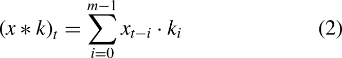
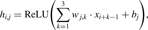
Convolutional Neural Networks (CNNs) were introduced as a type of feedforward neural network that excels in tasks such as image processing and natural language processing (NLP) (Shahriar, 2021). CNNs have also proven effective in time series prediction (Wibawa et al., 2022). The ability of CNNs to utilize local connectivity and weight sharing reduces the number of parameters, leading to more efficient learning models. A typical CNN architecture consists of three primary components: convolutional layers, pooling layers, and fully connected layers (Mann & Kalidindi, 2022). Each convolutional layer comprises multiple convolutional kernels, with the operation of these layers described by equation (1). The convolutional layers extract features from the input data, but this often results in high-dimensional feature maps. Therefore, to address this thus decreasing the computational cost, pooling layers are employed after the convolutional layers to reduce the dimensionality of the features (Zhao et al., 2024) (Figure 1)

Figure 1.

CNN architecture (Shahriar, 2021).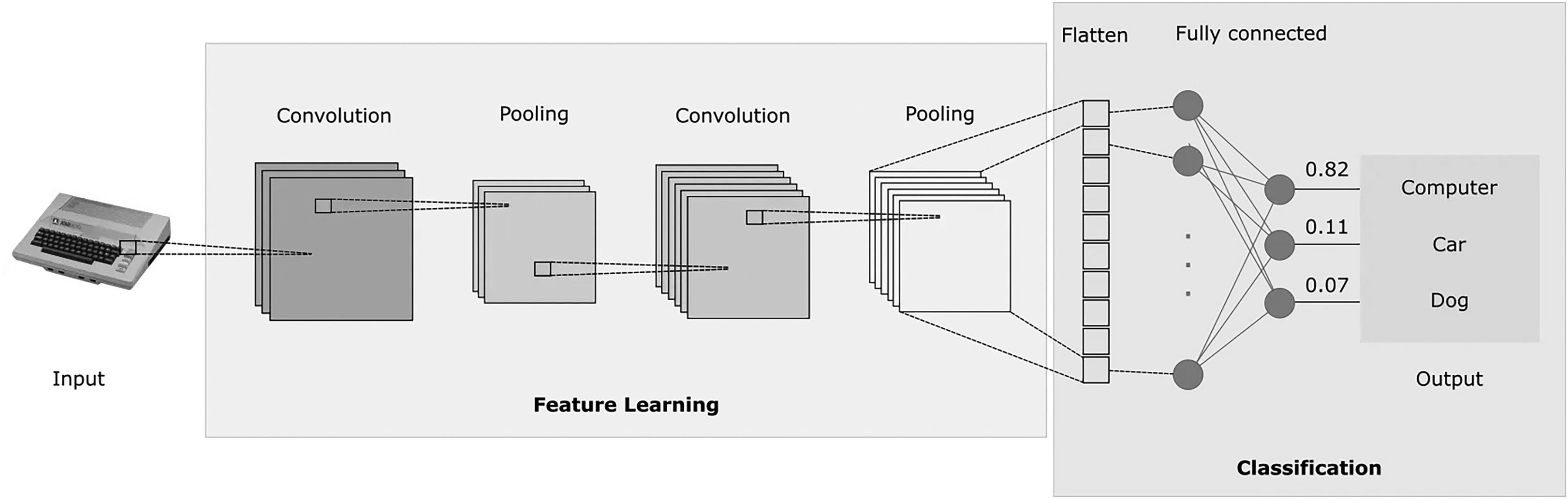

l_{t} = \tanh ((x * k)_{t} + b_{t})

(1)

In this equation, $l_{t}$ represents the output at time step $t$ after applying the convolution, $\tanh$ is the activation function, $x$ is the input vector, $k$ denotes the convolution kernel weights, and $b_{t}$ is the bias associated with the convolution kernel. In addition, the convolution operation $(x * k)_{t}$ for a 1D input sequence can be expressed as:

(x * k)_{t} = \sum_{i = 0}^{m - 1} x_{t - i} \cdot k_{i}

(2)

Accordingly,

m

is the size of the kernel,

x_{t - i}

is the input at the

i

-th position relative to the current time step

t

, and

k_{i}

are the kernel weights at the

i

-th position.

Long Short-Term Memory

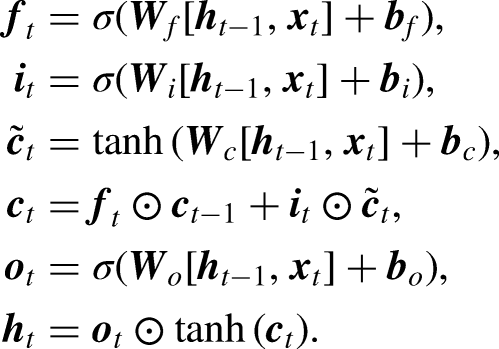
Long Short-Term Memory (LSTM), introduced by Hochreiter and Schmidhuber (1997), was designed to address the challenges of gradient explosion and vanishing gradients in Recurrent Neural Networks (RNNs) (Zucchet & Orvieto, 2024). Unlike the standard RNN, which consists of a single repeating tanh module, LSTM includes four interactive components, making it more effective in capturing long-term dependencies (Hochreiter & Schmidhuber, 1997). Accordingly, the core of LSTM is its memory cell, which is regulated by three gates: the forget gate, the input gate, and the output gate. These gates control the flow of information and update the cell state, which are outlined as follows (Figure 2):

The forget gate determines what portion of the previous cell state $C_{t - 1}$ should be retained, calculated as:

f_{t} = σ (W_{f} \cdot [h_{t - 1}, x_{t}] + b_{f})

(3)

where

σ

is the activation function,

W_{f}

and

b_{f}

are the weights and bias of the forget gate, respectively.

The input gate updates the cell state with new information, determined by:

i_{t} = σ (W_{i} \cdot [h_{t - 1}, x_{t}] + b_{i})

(4)

{\tilde{C}}_{t} = \tanh (W_{c} \cdot [h_{t - 1}, x_{t}] + b_{c})

(5)

where

i_{t}

is the input gate output, and

{\tilde{C}}_{t}

is the candidate cell state.

The cell state $C_{t}$ is updated by combining the forget gate and input gate:

C_{t} = f_{t} \cdot C_{t - 1} + i_{t} \cdot {\tilde{C}}_{t}

(6)

The output gate decides the next hidden state $h_{t}$ by:

o_{t} = σ (W_{o} \cdot [h_{t - 1}, x_{t}] + b_{o})

(7)

Finally, the output of the LSTM is computed as:

h_{t} = o_{t} \cdot \tanh (C_{t})

(8)

Figure 2.

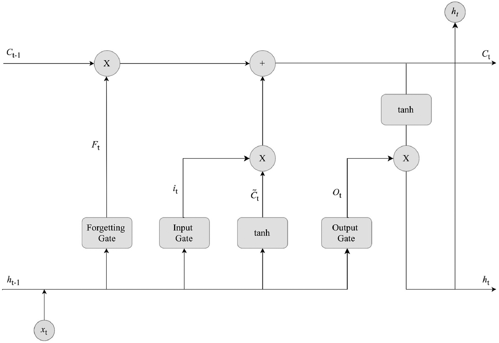
LSTM architecture.

$x_{t}$ represents the current input, $h_{t - 1}$ is the previous hidden state, and $b$ terms denote biases for the respective gates.

Attention Mechanism

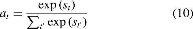
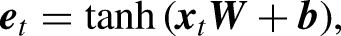
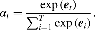
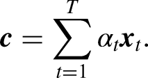
The Attention Mechanism (AM), introduced by Treisman and Gelade (1980), optimizes models by focusing on the most relevant information within large datasets. By calculating the probability distribution of attention, AM highlights key inputs, effectively enhancing traditional models based on human visual attention principles. This mechanism prioritizes important information while disregarding less relevant details, thus efficiently allocating attention. The AM calculation process, as illustrated in Figure 3, can be divided into three main stages:

The similarity between the Query (output feature) and Key (input feature) is calculated using:

s_{t} = \tanh (W_{h} h_{t} + b_{h})

(9)

where

W_{h}

is the weight matrix,

b_{h}

is the bias vector of the attention mechanism, and

h_{t}

is the input vector (or Key) at time step

t

. This computes a raw score

s_{t}

, representing the similarity between the Query and Key.

The similarity score $s_{t}$ is then normalized via the softmax function to obtain the attention weights:

a_{t} = \frac{\exp (s_{t})}{\sum_{t^{'}} \exp (s_{t^{'}})}

(10)

Accordingly,

a_{t}

represents the attention weight for the input at time step

t

. The softmax function ensures that the attention weights form a probability distribution, where

\sum_{t} a_{t} = 1

. This step allows the model to assign higher weights to more relevant inputs.

The final attention value is calculated through a weighted summation over all the input vectors (or Values):

s = \sum_{t} a_{t} h_{t}

(11)

In equation 11,

s

is the context vector that aggregates the input information, with each input

h_{t}

weighted by its corresponding attention weight

a_{t}

, which is used in subsequent computations to make predictions.

Figure 3.

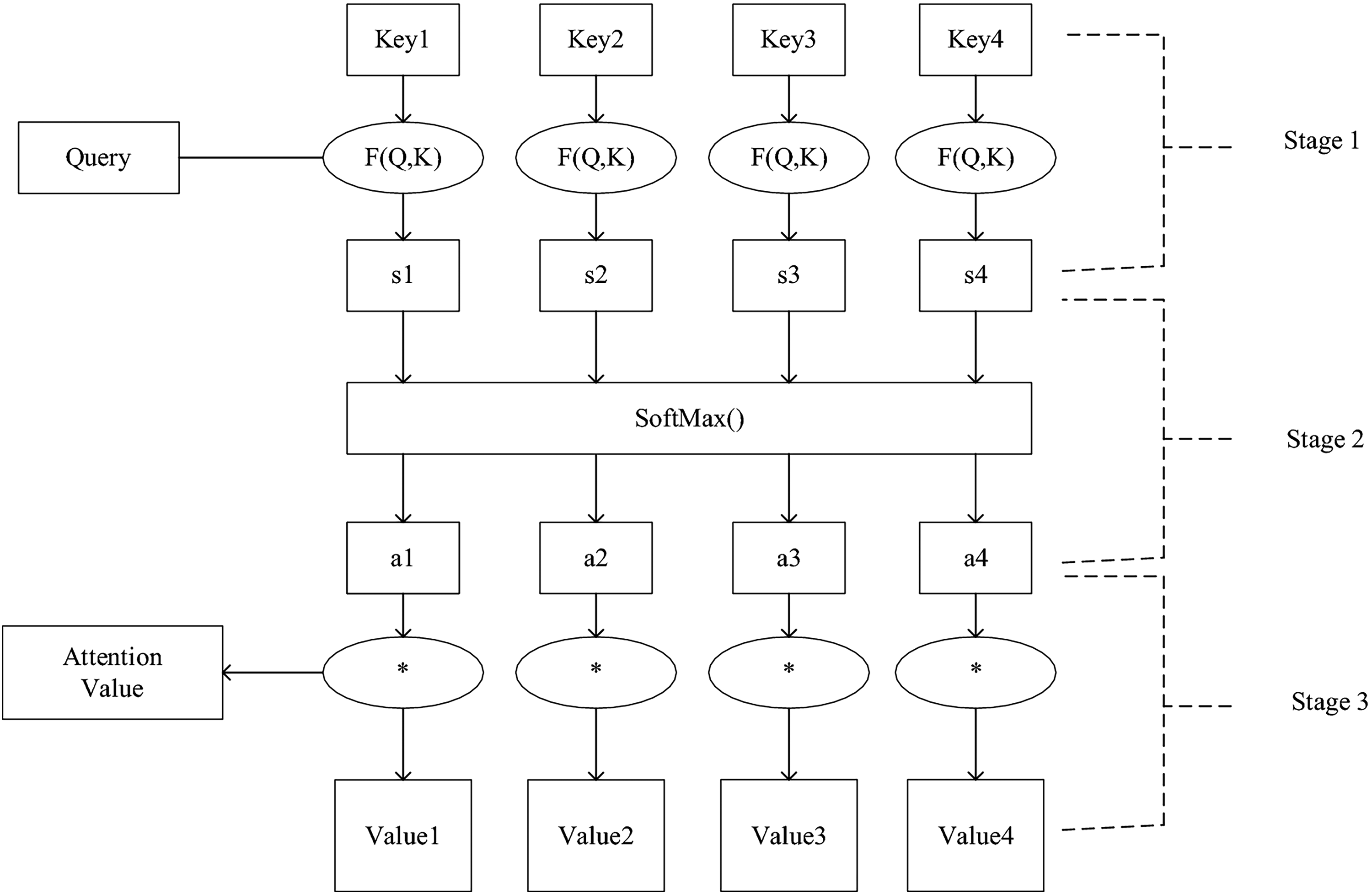
AM architecture (Lu et al., 2020).

Methodology

Data Collection and Evaluation Metrics

The OHLCV stock data, sourced from Yahoo Finance’s S&P 500 Index, are categorized into two groups: Pharmaceuticals (AbbVie Inc., ABBV; Johnson & Johnson, JNJ) and Financials (Goldman Sachs Group Inc., GS; Citigroup Inc., C). This categorization is based on the fundamental differences between pharmaceutical companies and financial institutions, presenting a unique challenge for forecasting models. Pharmaceutical stocks are sensitive to abnormal events (e.g., lab innovations, private research, cure development), whereas financial stocks are more influenced by periodic events (e.g., political debates, fiscal policies, human psychology). Additionally, CLAM employs a standard train-validate-test split ratio of 80:10:10. This means 80% of the data is used for initial training, 10% for validation and fine-tuning, and the remaining 10% for testing. The dataset’s timeline is structured with a train/val/test period from July 19, 2004, to July 12, 2024 (20 years - 5,031 observations). We then provide an out-of-sample forecast starting on July 13, 2024, predicting the next financial week, to justify CLAM’s prowess. Consequently, the out-of-sample (OOS) period spans July 15, 2024, to July 19, 2024 (5 observations). The OSS dataset was gathered separately from others.

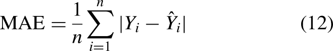
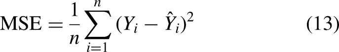
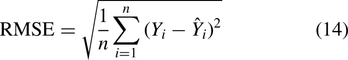
The experiment concludes on July 20, 2024, ensuring that the data remains unseen during training to fully avoid the possibility of data leakage. The Mean Absolute Error (MAE) and Root Mean Squared Error (RMSE) are selected as evaluation metrics due to their effectiveness in identifying predictive errors in univariate analysis. MAE (12) provides the average magnitude of forecasting errors, serving as a straightforward measure of overall prediction accuracy, which is particularly crucial in the volatile stock market. RMSE (13), on the other hand, emphasizes larger errors, highlighting discrepancies that could have significant financial consequences. Mean Squared Error (MSE) is used as the loss function to measure the average squared difference between the predicted values and the actual target values, quantifying the model’s prediction accuracy. Thus, greater errors indicate a larger deviation in price predictions.

MAE = \frac{1}{n} \sum_{i = 1}^{n} | Y_{i} - {\hat{Y}}_{i} |

(12)

MSE = \frac{1}{n} \sum_{i = 1}^{n} (Y_{i} - {\hat{Y}}_{i})^{2}

(13)

RMSE = \sqrt{\frac{1}{n} \sum_{i = 1}^{n} (Y_{i} - {\hat{Y}}_{i})^{2}}

(14)

Where:

$n$ is the total number of data points or observations.

$Y_{i}$ represents the actual (true) value of the stock price.

${\hat{Y}}_{i}$ represents the predicted value of the stock price.

CLAM: CNN-LSTM-AM

Overall, the synergistic design of CLAM, accumulating triple-stacked layers of CNN, LSTM, and a customized AM layer, enables the model to systematically extract local patterns, learn temporal dependencies, and focus on the most critical information in the sequence. Each component is carefully configured to address the unique challenges posed by financial time-series data, such as non-linearity, volatility, and nonstationarity across various data nature (Figure 4).

Figure 4.

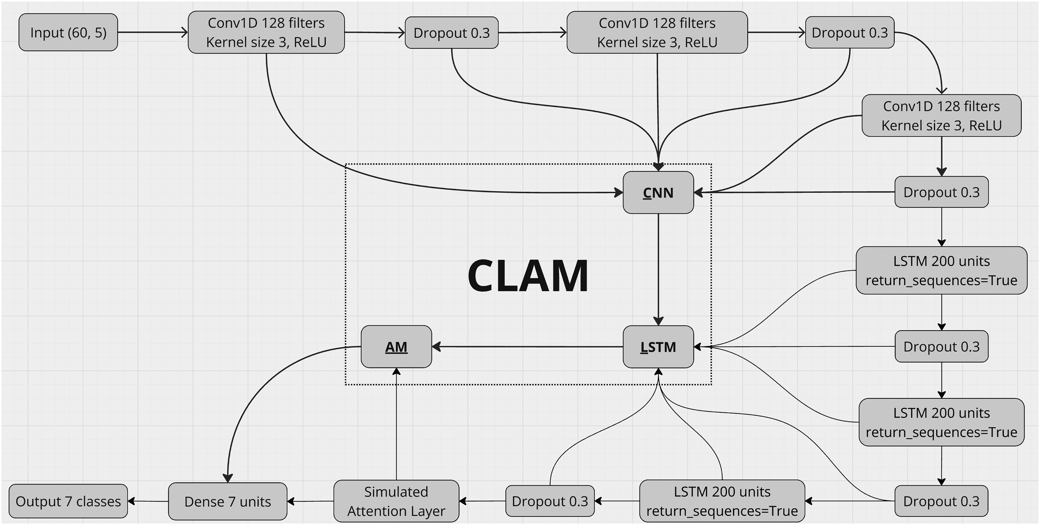
The proposed CLAM hybrid architecture.

Firstly, the input data, which includes normalized features including Open, High, Low, Adj Close, and Volume, is transformed into sequences of length 60 and passed through a series of three 1D Convolutional layers. These layers, each equipped with 128 filters and a kernel size of 3, scan the input sequences to detect localized spatial patterns over short temporal windows. For example, changes in price movements within three consecutive time steps may highlight emerging trends or market anomalies. Mathematically, the convolution operation computes feature maps at each step, defined as:

h_{i, j} = ReLU (\sum_{k = 1}^{3} w_{j, k} \cdot x_{i + k - 1} + b_{j}),

Accordingly,

w_{j, k}

and

b_{j}

represent the trainable weights and bias of the

j

-th filter. The activation function,

ReLU (z) = max (0, z)

, is applied to introduce non-linearity while retaining computational efficiency. However, convolution alone may overfit to noise or minor variations in the data. To address this, Dropout regularization with a rate of 0.3 follows each convolutional layer, stochastically deactivating a subset of neurons during training and promoting the generalization of extracted features. While the convolutional layers excel at capturing local spatial patterns, they lack the capability to model long-range temporal dependencies. This limitation is addressed by three stacked LSTM layers, each containing 200 units. These layers maintain an internal cell state to track dependencies over extended periods. At any given time step

t

, the LSTM cell calculates the updated cell state and hidden state through a series of gated operations:

\begin{aligned} f_{t} & = σ (W_{f} [h_{t - 1}, x_{t}] + b_{f}), \\ i_{t} & = σ (W_{i} [h_{t - 1}, x_{t}] + b_{i}), \\ {\tilde{c}}_{t} & = \tanh (W_{c} [h_{t - 1}, x_{t}] + b_{c}), \\ c_{t} & = f_{t} ⊙ c_{t - 1} + i_{t} ⊙ {\tilde{c}}_{t}, \\ o_{t} & = σ (W_{o} [h_{t - 1}, x_{t}] + b_{o}), \\ h_{t} & = o_{t} ⊙ \tanh (c_{t}) . \end{aligned}

Here, the forget gate (

f_{t}

) decides which parts of the previous cell state to retain, while the input gate (

i_{t}

) and candidate memory (

{\tilde{c}}_{t}

) determine how new information should influence the state. This mechanism allows the LSTM layers to dynamically adapt their memory based on evolving patterns. Stacking multiple LSTM layers enables the model to construct a hierarchical understanding of these temporal dependencies. As with the convolutional layers, Dropout is consistently applied at a rate of 0.3 to prevent overfitting. Next, the output from the LSTM layers is then passed to the Attention Mechanism, which acts as a filter to emphasize the most relevant time steps for the forecasting task. Unlike traditional sequence models, where all time steps are treated equally, the attention mechanism learns to assign importance weights, or attention scores, to each time step. These scores are computed as:

e_{t} = \tanh (x_{t} W + b),

and normalized using the softmax function:

α_{t} = \frac{\exp (e_{t})}{\sum_{i = 1}^{T} \exp (e_{i})} .

The resulting weights

α_{t}

indicate the contribution of each time step to the final prediction. The model computes a context vector by aggregating the weighted inputs:

c = \sum_{t = 1}^{T} α_{t} x_{t} .

This vector captures the most critical information in the sequence, ensuring that the model prioritizes influential patterns while ignoring irrelevant details. Finally, the context vector is processed by a Dense layer with 7 output units, corresponding to the 7-day forecast horizon. The dense layer applies a linear transformation:

\hat{y} = W_{out} c + b_{out},

This maps the learned features to the predicted stock prices. This end-to-end pipeline spans spatial extraction, temporal modelling, and context-aware attention. All demonstrate the ability of the CLAM in handling the complexities of financial time-series data. Further hyperparemeter-tuning processes on these layers and their components (Tables 1 and 2) would help CLAM to achieve a balance between expressive power and generalizability. This lightweight architecture ensures CLAM’s effectiveness in real-world forecasting scenarios, as supported by its performance metrics in Table 3.

Table 1.

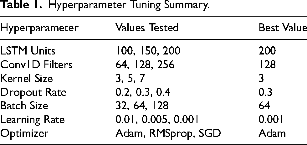
Hyperparameter Tuning Summary.

Hyperparameter	Values Tested	Best Value
LSTM Units	100, 150, 200	200
Conv1D Filters	64, 128, 256	128
Kernel Size	3, 5, 7	3
Dropout Rate	0.2, 0.3, 0.4	0.3
Batch Size	32, 64, 128	64
Learning Rate	0.01, 0.005, 0.001	0.001
Optimizer	Adam, RMSprop, SGD	Adam

Table 2.

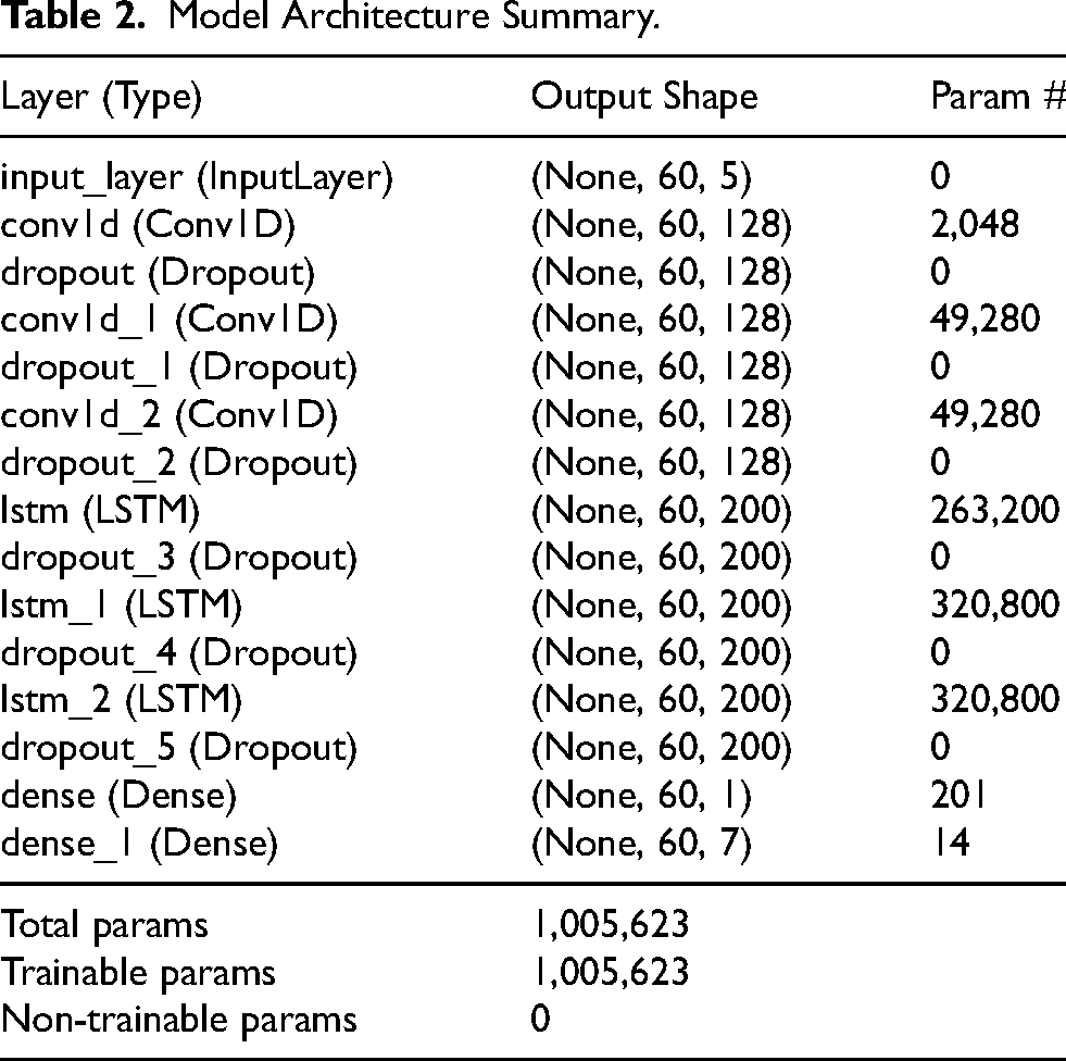
Model Architecture Summary.

Layer (Type)	Output Shape	Param #
input_layer (InputLayer)	(None, 60, 5)	0
conv1d (Conv1D)	(None, 60, 128)	2,048
dropout (Dropout)	(None, 60, 128)	0
conv1d_1 (Conv1D)	(None, 60, 128)	49,280
dropout_1 (Dropout)	(None, 60, 128)	0
conv1d_2 (Conv1D)	(None, 60, 128)	49,280
dropout_2 (Dropout)	(None, 60, 128)	0
lstm (LSTM)	(None, 60, 200)	263,200
dropout_3 (Dropout)	(None, 60, 200)	0
lstm_1 (LSTM)	(None, 60, 200)	320,800
dropout_4 (Dropout)	(None, 60, 200)	0
lstm_2 (LSTM)	(None, 60, 200)	320,800
dropout_5 (Dropout)	(None, 60, 200)	0
dense (Dense)	(None, 60, 1)	201
dense_1 (Dense)	(None, 60, 7)	14
Total params	1,005,623
Trainable params	1,005,623
Non-trainable params	0

Experiments and Results

Experimental Process

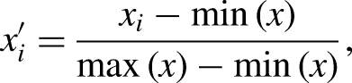
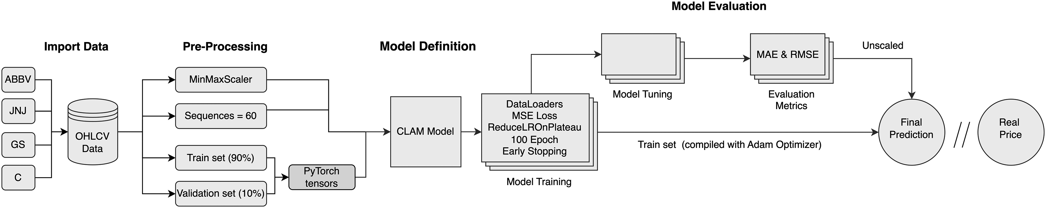
Our experimental procedure (Figure 5) began with the initialization of random number generators in both NumPy and TensorFlow libraries, ensuring consistency and reproducibility by setting a seed value of 42. The stock datasets, loaded from csv files, contained OHLCV data, which were first normalized to address varying magnitudes among features. Two separate MinMaxScaler instances were used: one for the feature columns (Open, High, Low, Adj Close, Volume) and another for the target column (Close). This process ensured that all values were scaled uniformly within the $[- 1, 1]$ range, reducing potential biases and enhancing the model’s numerical stability. The normalization for a given feature was computed as:

x_{i}^{'} = \frac{x_{i} - min (x)}{max (x) - min (x)},

Accordingly,

x_{i}

represents the original value, and

min (x)

and

max (x)

denotes the minimum and maximum values of the feature across the dataset. After normalization, sequences were constructed from the dataset to model temporal dependencies. Each sequence covered 60 consecutive days as input and was used to predict the subsequent 7 days of closing prices. The input-output pairs were derived exclusively from the normalized dataset to prevent any leakage of future information, maintaining the integrity of the forecasting setup. Formally, for a sequence starting at index

i

, the input and output were defined as:

X_{i} = [x_{i}, x_{i + 1}, \dots, x_{i + 59}], y_{i} = [x_{i + 60}, x_{i + 61}, \dots, x_{i + 66}] .

This sequence creation process yielded a substantial number of training samples, which were then split into training and validation sets in a 90:10 ratio. This split ensured that the model was evaluated on unseen data, mitigating overfitting and providing an accurate measure of its generalization capability. The model architecture, designed to capture both spatial and temporal patterns, began with convolutional layers to extract localized spatial features from the input sequences. Each Conv1D layer consisted of 128 filters with a kernel size of 3, enabling the detection of short-term patterns within the data. The outputs of these layers were then passed through three stacked LSTM layers, each with 200 units, to model long-term temporal dependencies. These LSTM layers maintained internal memory states, allowing the model to learn evolving trends over extended periods. Following the LSTM layers, an Attention mechanism was introduced to prioritize critical time steps within the sequences. The attention mechanism assigned weights,

α_{t}

, to each time step based on its relevance to the prediction. This process allowed the model to focus on the most important information, enhancing its ability to make accurate forecasts. The model was trained using a batch size of 64, which balanced computational efficiency and convergence stability. A ReduceLROnPlateau scheduler dynamically adjusted the learning rate, reducing it by a factor of 0.2 if the validation loss did not improve for 5 consecutive epochs, with a minimum learning rate set to 0.001.

Figure 5.

Full experimental process.

In addition, EarlyStopping was employed, halting the training process if the validation loss did not improve after 10 epochs. These strategies ensured that the model avoided overfitting while training efficiently. Throughout training, the model iterated over the dataset in batches, updating weights via backpropagation after each batch. The early stopping criterion ensured that the model retained its best weights based on validation performance. After training, the model was evaluated on the validation set, with metrics such as MAE and RMSE providing insights into its predictive accuracy. Finally, the trained model was used to generate out-sample forecasts, which were unscaled using the inverse transformation of the MinMaxScaler. This final step restored the predictions to their original value range, facilitating direct comparison with the test data and validating the model’s effectiveness in real-world scenarios.

Hyperparameter Tuning

As illustrated in Table 1, a wide spectrum of values was tested across essential hyperparameters, including LSTM units, Conv1D filters, kernel size, dropout rate, batch size, learning rate, and optimizer selection. This exhaustive tuning process was essential to strike the delicate balance between model complexity and generalization, with a specific focus on avoiding overfitting, a common pitfall in deep learning models. The selection of 200 LSTM units, for instance, was the result of a careful trade-off. While a smaller number of units (such as 100 or 150) led to faster convergence, these configurations consistently underperformed in capturing the complexity of the sequential data, as evidenced by higher validation errors. Conversely, larger configurations, such as 256 Conv1D filters, introduced unnecessary computational overhead without a commensurate improvement in performance, highlighting the diminishing returns of increasing model depth and width. In addition, the kernel size of 3 was particularly effective in capturing localized temporal patterns, contrasting with larger kernels that diluted the model’s ability to focus on fine-grained features.

Moreover, the dropout rate of 0.3 was determined to be optimal after observing that lower rates led to overfitting, while higher rates hindered learning, reducing the model’s capacity to generalize. The choice of a batch size of 64 was similarly contrasted against smaller and larger batch sizes, where smaller batches resulted in noisier gradient estimates and larger batches slowed down the training without significant gains in accuracy. The learning rate of 0.001, coupled with the Adam optimizer, offered the best balance between learning speed and stability, particularly when compared to other optimizers like RMSprop and SGD, which either converged slower or required more tuning.

Performance Comparison

The results in Table 3 confirm CLAM as the top-performing model across all datasets and metrics. For ABBV, the MAE of 0.008 represents a 90.9% reduction compared to LSTM-AM’s 0.088 and an impressive 93.2% over CNN’s 0.117. While LSTM-AM improves upon CNN-LSTM by 16.2% and CNN by 24.8%, its gains are modest compared to CLAM. On the C dataset, the MAE of 0.012 surpasses LSTM-AM’s 0.097 by 87.6% and CNN-LSTM’s 0.115 by 89.6%. Even with attention mechanisms, LSTM-AM reduces CNN’s error by only 28.1% (0.135 to 0.097), falling short of the reductions achieved by CLAM. For GS, CLAM achieves a MAE of 0.017, 81.3% lower than LSTM-AM’s 0.091 and 86.9% better than CNN’s 0.130. The JNJ dataset, characterized by lower overall errors, still highlights CLAM’s effectiveness. Its MAE of 0.019 reduces errors by 78.9% relative to LSTM-AM and 83.5% compared to CNN. These patterns demonstrate CLAM’s ability to capture temporal dependencies and adapt across datasets.

Table 3.

Model Performance on Train and Test Sets.

Model	ABBV		C		GS		JNJ
	Validation	Test	Validation	Test	Validation	Test	Validation	Test
MAE
CNN (Akşehýr & Kılıç, 2022)	0.114	0.117	0.139	0.135	0.128	0.130	0.107	0.115
LSTM (Al-Utaibi et al., 2023)	0.130	0.135	0.149	0.151	0.154	0.157	0.127	0.134
CNN-LSTM (Liu et al., 2022)	0.010	0.105	0.110	0.115	0.099	0.107	0.094	0.102
LSTM-AM (Chen et al., 2023)	0.082	0.088	0.093	0.097	0.091	0.096	0.083	0.090
CLAM	0.019	0.008	0.012	0.020	0.017	0.024	0.032	0.019
RMSE
CNN (Akşehýr & Kılıç, 2022)	0.141	0.147	0.185	0.187	0.173	0.176	0.130	0.137
LSTM (Al-Utaibi et al., 2023)	0.158	0.161	0.190	0.195	0.21	0.27	0.161	0.167
CNN-LSTM (Liu et al., 2022)	0.122	0.128	0.139	0.144	0.132	0.143	0.121	0.128
LSTM-AM (Chen et al., 2023)	0.108	0.115	0.125	0.129	0.118	0.125	0.110	0.116
CLAM	0.025	0.033	0.019	0.025	0.023	0.034	0.025	0.026

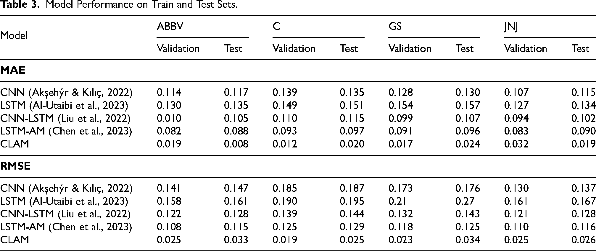
RMSE metrics reinforce these trends. For ABBV, the RMSE of 0.025 is 77.5% lower than LSTM-AM and 83.0% below CNN. On C, it outperforms LSTM-AM by 79.4% and CNN by 86.5%. GS and JNJ datasets show similar advantages, with reductions exceeding 80% over LSTM-AM and CNN. Although LSTM-AM offers significant improvements over simpler models, it consistently lags behind CLAM, which delivers unmatched accuracy and robustness. CLAM remains unmatched in precision and consistency among others. Results show diverse gaps between validation and test results. An inspection of the error metrics was conducted to justify CLAM efficient training.

CLAM Inspection

Training and Validation

The training process (Figure 6) for ABBV shows effective learning, with MAE dropping from 0.10 to 0.025 by epoch 20, and validation MAE stabilizing around 0.025 by epoch 65. RMSE decreases from 0.16 to below 0.04, indicating strong generalization. For stock C, the training MAE quickly declines from 0.045 to 0.020 by epoch 10, while validation MAE stabilizes around 0.015 by epoch 30. Both MAE and RMSE converge near 0.010 and 0.02, respectively, by epoch 60, reflecting robust learning. In GS, training MAE drops to 0.03 by epoch 10, with validation MAE stabilizing at 0.02 by epoch 30. RMSE similarly decreases below 0.03, confirming effective model performance. For JNJ, the training MAE drops to 0.03 by epoch 5, with validation MAE stabilizing around 0.03 by epoch 10. RMSE decreases to 0.04 from epoch 10 onward, showing effective learning dynamics.

Figure 6.

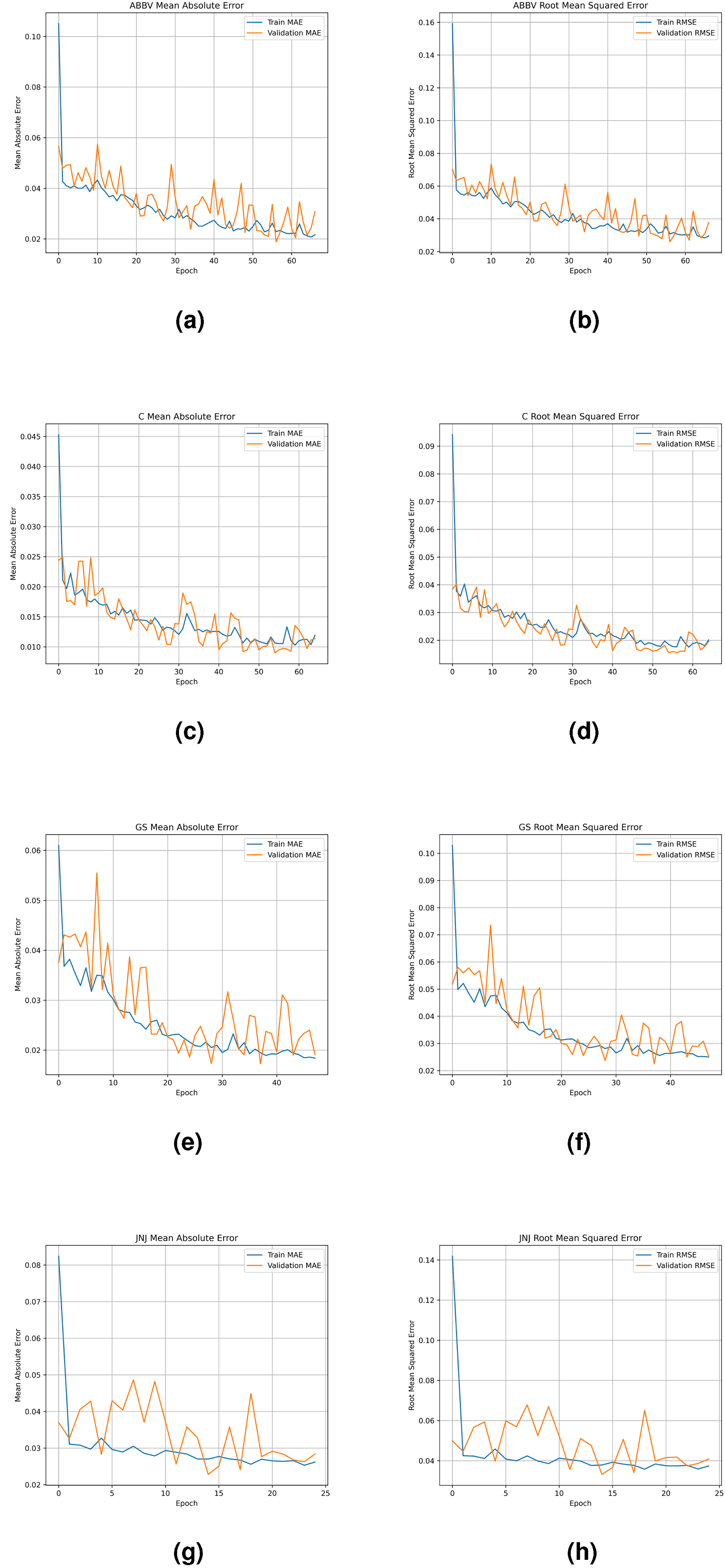
Summary of MAE and RMSE for different datasets. (a) MAE of ABBV; (b) RMSE of ABBV; (c) MAE of C; (d) RMSE of C; (e) MAE of GS; (f) RMSE of GS; (g) MAE of JNJ and (h) RMSE of JNJ.

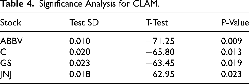
Table 4 evaluates the CLAM’s performance by analyzing Standard Deviation (SD) (Rowberry, 2021), T-Test (Emerson, 2023), and P-Value (Kwak, 2023) between the test sets and the actual sets of stocks. For ABBV, CLAM achieves a Test SD of 0.010, a strongly negative T-Test value of $- 71.25$ , and a P-Value of 0.009. These metrics indicate both high precision and statistically significant performance. The C dataset, which is more volatile, shows a slightly higher Test SD of 0.020. However, the T-Test of $- 65.80$ and a P-Value of 0.013 still demonstrate that CLAM effectively handles noisier time series data. For GS and JNJ, the Test SDs are 0.023 and 0.018, respectively, accompanied by T-Test values of $- 63.45$ and $- 62.95$ . Both datasets yield P-Values well below 0.05, confirming the model’s reliability across varying conditions. Overall, despite minor deviations, CLAM’s statistical performance in financial time series forecasting shows stable accuracy, adaptability, and statistical significance, even in challenging financial datasets.

Table 4.

Significance Analysis for CLAM.

Stock	Test SD	T-Test	P-Value
ABBV	0.010	$- 71.25$	0.009
C	0.020	$- 65.80$	0.013
GS	0.023	$- 63.45$	0.019
JNJ	0.018	$- 62.95$	0.023

Trend Forecasting

Finally, CLAM is deployed into real-world scenarios for outsample forecasting generation (Figure 7), then contrasted with the end-period value in the OOS dataset. By leveraging historical price patterns, CLAM aims to capture shifts in market momentum, labelling trends as “UP” if the next day’s price is expected to rise and “DOWN” if it is expected to fall. This approach reduces the influence of short-term noise.

Figure 7.

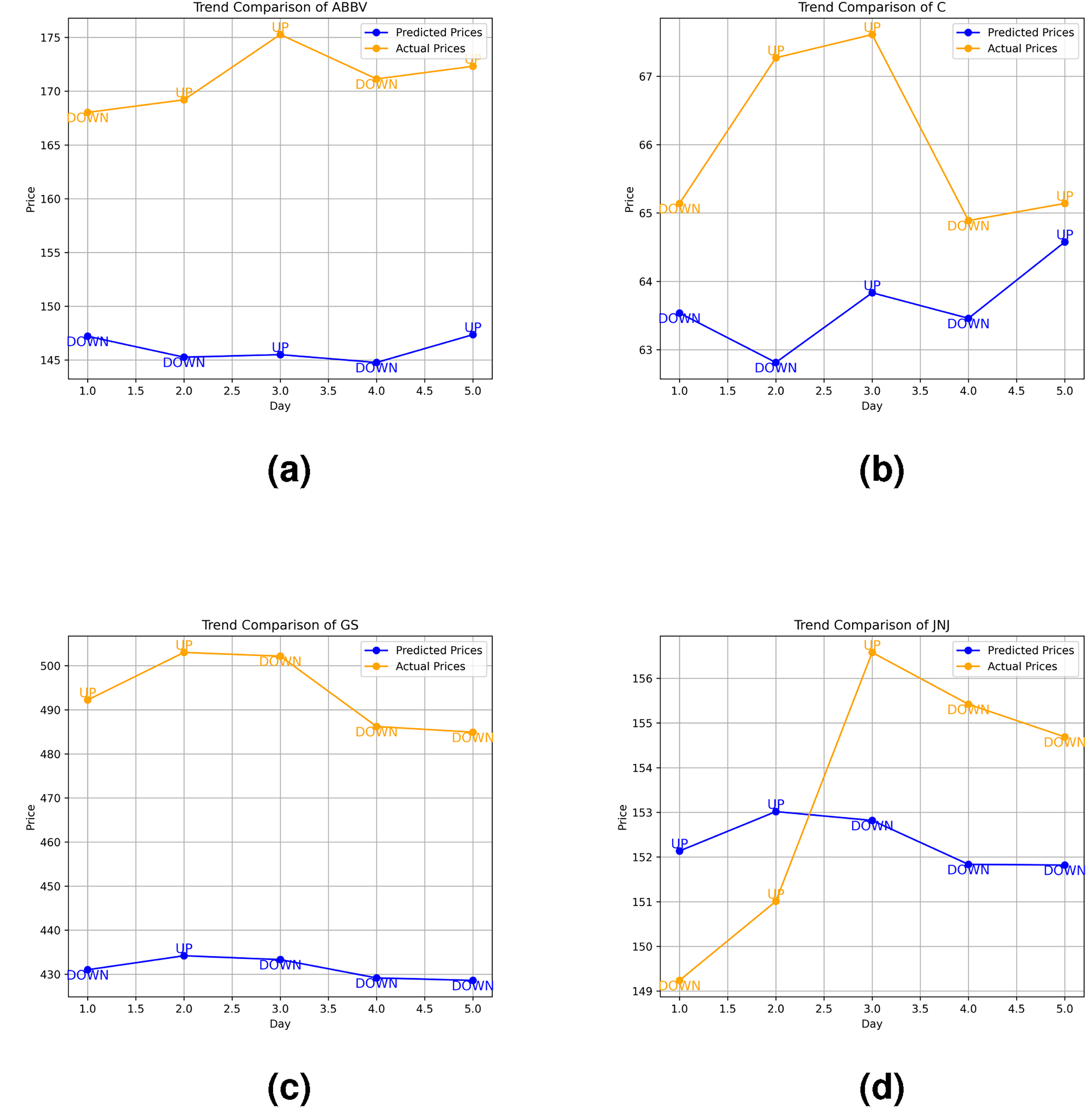
Forecasting results for stocks. (a) ABBV forecasting results; (b) C forecasting results; (c) GS forecasting results and (d) JNJ forecasting results.

For ABBV, CLAM successfully identified the immediate downtrend on Day 1 (Monday), a day typically marked by high volatility and investor reactions post-weekend. Although it initially missed the recovery on Day 2, it adjusted and accurately predicted the upward trend on Day 3. CLAM then continued to forecast the correct trend for the final two days, resulting in three consecutive accurate predictions and capturing the overall uptrend of ABBV, achieving an accuracy of 80%. In the case of C, CLAM once again identified the initial downtrend on Monday but failed to predict the following day’s trend. However, it redeemed by precisely forecasting the trend for the last three days consecutively, with minimal price deviation, leading to an overall accuracy of 80%. Concerning GS’s case, despite missing the initial rise on Day 1 (after the weekend), CLAM consistently predicted the correct trend for the remaining four consecutive days, successfully capturing the overall downtrend for the week and once again achieving 80% accuracy. Finally, for JNJ, while CLAM effectively captured the overall downward trend, it struggled with consistency, failing to predict the trends on Days 1 and 3. Nevertheless, it accurately captures the sharp decline in the final two days, resulting in a 60% accuracy for JNJ.

Overall, CLAM achieved an average trend forecasting accuracy of 75% across pharmaceutical and finance stocks. The model demonstrated strong performance in most cases, particularly in forecasting consecutive trends, and identifying immediate downtrends. The test was conducted as proof of CLAM’s promising applicability in real-time intraday trading systems. As outsample data did not exist during the training and forecasting processes, the remarkable output could have optimized investors’ trading portfolios by alerting a hold, buy, or sell position (Dichtl, 2018) one week ahead of the S&P 500 market, reducing investment risks.

Discussion

Summary of Findings and Contributions

Our research demonstrates that the integration of stacked deep learning layers in the CLAM model, comprising Convolutional Neural Networks (CNN), Long Short-Term Memory (LSTM), and Attention Mechanisms (AM), significantly outperforms traditional standalone models. This superiority is attributed to CLAM’s advanced feature extraction and attention mechanisms, which enhance the LSTM architecture’s inherent ability to capture long-term dependencies in time series forecasting. As a result, CLAM achieves an average reduction of over 80% in MAE and RMSE compared to conventional models such as CNN, LSTM, CNN-LSTM, and LSTM-AM. Additionally, our experiments indicate that in 3 out of 4 cases, CLAM successfully forecasts the correct trends for 3-4 consecutive days, capturing market downturns on the opening day, which tends to be unpredictable due to abnormal traders’ behaviour.

Finally, CLAM achieves a 75% accuracy rate in stock trend forecasting. This highlights the potential of hybrid models in time series forecasting, demonstrating that attention-based deep learning hybrids like CLAM are particularly well-suited as live-trading indicators for investors focused on weekly trends. Hence, CLAM enhances decision-making processes in financial trading, providing a robust and lightweight tool to forecast short-term movements in the global equity market.

Limitations and Recommendations

Our study is grounded in raw OHLCV data of stock prices, which offers ease of access but also introduces potential market biases. This limitation arises from the model’s inability to account for external economic or financial factors, such as extreme events, technical indicators, or government policies, all of which are crucial drivers of stock prices. Additionally, since our research primarily focuses on trend detection, the CLAM architecture is not fully optimized for value trading, where precise price gaps are critical. As a result, CLAM’s potential may extend further and be more robust than demonstrated in its current form. We encourage researchers to expand upon our work by developing deeper hybrid models or employing explainable models to study stock trends effectively. In addition, practitioners are advised to enhance data collection processes by incorporating data from stock indexes and integrating relevant technical trading indicators, thereby uncovering more intricate stock patterns within the raw target features.

Conclusion

This study introduced the CLAM model, a hybrid combination of Convolutional Neural Networks, Long Short-Term Memory networks, and Attention Mechanisms designed for multi-step stock price trend forecasting. The model demonstrated significant improvements in predictive accuracy, with an average reduction of over 80% in MAE and RMSE compared to traditional models. CLAM’s ability to effectively capture complex temporal dependencies and its robust performance across various stock datasets highlight its potential as a valuable tool in financial forecasting. The findings of this research suggest that CLAM is particularly well-suited for short-term trend forecasting, providing accurate and timely predictions that can assist investors and traders in making informed decisions.

The model’s design, which integrates feature extraction and attention mechanisms, offers a significant advancement over existing approaches. Moreover, there are several promising directions for further research. Future studies could explore enhancing CLAM’s adaptability to different market conditions, such as varying levels of market volatility or the impact of external economic factors. Integrating CLAM with other financial analysis techniques, such as sentiment analysis or candlestick pattern recognition, could also improve its predictive capabilities. Real-time deployment of CLAM in live trading environments of daily stocks or hourly cryptocurrency prices is another area that warrants investigation for real-time performance assessment.

Footnotes

ORCID iD

Nguyen Quoc Anh

Funding

The author(s) received no financial support for the research, authorship, and/or publication of this article.

Declaration of Conflicting Interests

The author(s) declared no potential conflicts of interest with respect to the research, authorship, and/or publication of this article.

References

Akşehýr

Z. D.

Kılıç

(2022). How to handle data imbalance and feature selection problems in CNN-based stock price forecasting. IEEE Access, 10, 31297–31305.

Al-Utaibi

K. A. A.

Siddiq

Sait

S. M.

(2023). Stock price forecasting with LSTM: A brief analysis of mathematics behind LSTM. Biophysical Reviews and Letters, 19(4), 361–371.

Anh

N. Q.

(2024a). A lightweight multi-head attention transformer for stock price forecasting. SSRN Electronic Journal, 1(1), 1–26.

Anh

N. Q.

(2024b). Transforming stock price forecasting: Deep learning architectures and strategic feature engineering. In Modeling decisions for artificial intelligence.

Anh

N. Q.

Thai

(2024). Phase space reconstructed neural ordinary differential equations model for stock price forecasting. In Pacific Asia conference on information systems.

Bahdanau

Cho

Bengio

(2014). Neural machine translation by jointly learning to align and translate. arXiv preprint arXiv:1409.0473.

Baker

Wurgler

(2006). Investor sentiment and the cross-section of stock returns. The Journal of Finance, 61(4), 1645–1680.

Bhuriya

Kaushik

Sharma

Singh

et al. (2017). Stock market prediction using a hybrid approach. In 2017 International conference on computing, communication and automation (ICCCA) (pp. 305–310).

Bikhchandani

Hirshleifer

Welch

(1992). A theory of fads, fashion, custom, and cultural change as informational cascades. Journal of Political Economy, 100(5), 992–1026.

10.

Box

G. E.

Jenkins

G. M.

Reinsel

G. C.

Ljung

G. M.

(2015). Time series analysis: Forecasting and control. John Wiley & Sons.

11.

Breiman

Friedman

Stone

C. J.

Olshen

R. A.

(1984). Classification and regression trees. CRC Press.

12.

Chen

Fang

Liang

Sha

Zhou

Song

(2021). Stock price forecast based on CNN-BILSTM-ECA model. Scientific Programming, 2021, 2446543:1.

13.

Chen

Leung

M. H.

Daouk

(2015). Forecasting the chinese stock market with a hybrid machine learning model. Journal of Empirical Finance, 29, 1–13.

14.

Chen

Zhan

(2023). Feature-ranked attention-driven LSTM: A novel hybrid model for short-term stock price predictions. In 2023 IEEE international symposium on product compliance engineering - Asia (ISPCE-ASIA) (pp. 1–6).

15.

Chong

E. K.

Han

Park

F. C.

(2017). Deep learning networks for stock market analysis and prediction: Methodology, data representations, and case studies. Expert Systems with Applications, 83, 187–205.

16.

Cont

(2001). Empirical properties of asset returns: Stylized facts and statistical issues. Quantitative Finance, 1(2), 223–236.

17.

De Gooijer

J. G.

Hyndman

R. J.

(2011). Forecasting using a hybrid SARIMA and support vector machines model: An application to UK electricity demand. International Journal of Forecasting, 27(3), 735–758.

18.

Dichtl

(2018). Investing in the S&P 500 index: Can anything beat the buy-and-hold strategy? ERN: Efficient Market Hypothesis Models (Topic), 38(2), 352–378.

19.

Emerson

R. W.

(2023). Mann-Whitney U test and t-test. Journal of Visual Impairment & Blindness, 117, 99–100.

20.

Esteva

Robicquet

Ramsundar

Kuleshov

DePristo

Chou

Cui

Corrado

G. S.

Thrun

Dean

(2019). A guide to deep learning in healthcare. Nature Medicine, 25(1), 24–29.

21.

Fama

E. F.

(1981). Stock returns, real activity, inflation, and money. The American Economic Review, 71(4), 545–565.

22.

Ferdus

M. Z.

Anjum

Nguyen

T. N.

Jisan

A. H.

Raju

M. A. H.

(2024). The influence of social media on stock market: A transformer-based stock price forecasting with external factors. Journal of Computer Science and Technology Studies, 6(1), 189–194.

23.

Kelly

Xiu

(2018). Empirical asset pricing via machine learning. arXiv preprint arXiv:1809.01078.

24.

Guan

Zhu

Xiao

(2023). Unveiling the predictive power: Comparative analysis of cutting-edge deep learning models for stock price forecasting. Highlights in Business, Economics and Management, 19(2), 17–29.

25.

Hagenau

Liebmann

Neumann

(2013). Automated news reading: Stock price prediction based on financial news using context-capturing features. Decision Support Systems, 55(3), 685–697.

26.

Ham

Y. G.

Kim

J. H.

Luo

J. J.

(2019). Deep learning for multi-year ENSO forecasts. Nature, 573(7775), 568–572.

27.

Hastie

Tibshirani

Friedman

(2009). The elements of statistical learning: Data mining, inference, and prediction. Springer.

28.

Henrique

B. M.

Sobreiro

V. A.

(2019). Literature review: Machine learning techniques applied to financial market prediction. Expert Systems with Applications, 124, 226–251.

29.

Hochreiter

Schmidhuber

(1997). Long short-term memory. Neural Computation, 9(8), 1735–1780.

30.

Luo

Xia

Yang

Liew

A. W. C.

(2024). Galformer: A transformer with generative decoding and a hybrid loss function for multi-step stock market index prediction. Scientific Reports, 14, 1–18.

31.

Kwak

S. K.

(2023). Are only p-values less than 0.05 significant? A p-value greater than 0.05 is also significant!. Journal of Lipid and Atherosclerosis, 12, 89–95.

32.

LeCun

Bengio

Hinton

(2015). Deep learning. Nature, 521(7553), 436–444.

33.

LeCun

Bottou

Bengio

Haffner

(1998). Gradient-based learning applied to document recognition. Proceedings of the IEEE, 86(11), 2278–2324.

34.

Liu

Shen

Wang

Chen

Huang

(2023). Master: Market-guided stock transformer for stock price forecasting. ArXiv abs/2312.15235.

35.

Wang

Shen

(2020). Deep learning-based stock index prediction: A comparative study. Applied Intelligence, 50(6), 3403–3416.

36.

Liaw

Wiener

(2002). Classification and regression by randomforest. R News, 2(3), 18–22.

37.

Lim

Oreshkin

B. N.

Bohdal

Ramos

Smyl

(2021). Temporal fusion transformers for interpretable multi-horizon time series forecasting. International Journal of Forecasting, 37(4), 1748–1764.

38.

Lipton

Z. C.

(2018). The mythos of model interpretability. Communications of the ACM, 61(10), 36–43.

39.

Liu

Qiao

Zhao

Keyao

Mei

Toe

T. T.

(2022). CNN-LSTM model stock forecasting based on an integrated attention mechanism. In 2022 3rd International conference on pattern recognition and machine learning (PRML) (pp. 403–408).

40.

Wang

Qin

(2020). A CNN-BiLSTM-AM method for stock price prediction. Neural Computing and Applications, 33, 4741–4753.

41.

Mahajan

Sinha

(2020). A hybrid SARIMA-XGBoost model and its application to forecasting indian stock index. Journal of Statistics and Management Systems, 23(1), 31–48.

42.

Mann

Kalidindi

S. R.

(2022). Development of a Robust CNN model for capturing microstructure-property linkages and building property closures supporting material design. In Frontiers in materials.

43.

Mantegna

R. N.

Stanley

H. E.

(1999). Introduction to econophysics: Correlations and complexity in finance. Cambridge University Press.

44.

Mikolov

Karafiát

Burget

Cernocký

Khudanpur

(2010). Recurrent neural network based language model. In Interspeech.

45.

Montgomery

D. C.

Peck

E. A.

Vining

G. G.

(2012). Introduction to linear regression analysis. John Wiley & Sons.

46.

Nguyen

Shirai

Velcin

(2015). Neural networks for financial time series forecasting: A review. Neural Computing and Applications, 25(2), 305–315.

47.

Pang

Zhou

Wang

(2020). Deep learning models for stock price prediction: A review. Journal of Forecasting, 39(4), 623–659.

48.

Porter

M. E.

(1985). Technology and competitive advantage. Harvard Business Review.

49.

Qin

Song

Chen

Cheng

Jiang

Cottrell

G. W.

(2017). A dual-stage attention-based recurrent neural network for time series prediction. In Proceedings of the 26th international joint conference on artificial intelligence (IJCAI) (pp. 2627–2633).

50.

Rowberry

(2021). Standard deviation (SD). In Encyclopedia of autism spectrum disorders.

51.

Shahriar

(2021). What is convolutional neural network (CNN)? Deep learning (accessed 18 August 2024).

52.

Sharif

Aloui

Yarovaya

(2021). COVID-19 pandemic: Impact of restriction policies on the economy. Environment, Development and Sustainability, 23(6), 9389–9412.

53.

Staffini

(2022). Stock price forecasting by a deep convolutional generative adversarial network. Frontiers in Artificial Intelligence, 5, 1–16.

54.

Treisman

Gelade

G. A.

(1980). A feature-integration theory of attention. Cognitive Psychology, 12, 97–136.

55.

Tsay

R. S.

(2005). Analysis of financial time series (Vol. 543). John Wiley & Sons.

56.

Vapnik

(1995). Support-vector networks. Springer.

57.

Vaswani

Shazeer

Parmar

Uszkoreit

Jones

Gomez

A. N.

Kaiser

Polosukhin

(2017). Attention is all you need. Advances in Neural Information Processing Systems, 30, 1–15.

58.

Wang

Lin

Zhang

Manos

(2019). Combining statistical and machine learning methods to predict financial time series. Journal of Computational Finance, 23(2), 1–20.

59.

Wang

Liu

Watada

(2024). Cross-modal scenario generation for stock price forecasting using Wasserstein GAN and GCN. Applied Soft Computing., 167, 112342.

60.

Wibawa

A. P.

Utama

A. B. P.

Elmunsyah

Pujianto

Dwiyanto

F. A.

Hernandez

(2022). Time-series analysis with smoothed convolutional neural network. Journal of Big Data, 9, 1–18.

61.

(2024). Comparative analysis of LSTM and transformer-based models for stock price forecasting. In AIP conference proceedings.

62.

Zeng

Chen

M. H.

Zhang

(2022). Are transformers effective for time series forecasting? In AAAI conference on artificial intelligence.

63.

Zhang

Wang

Zhang

(2017). A hybrid model based on CEEMDAN and GWO for stock price forecasting. Applied Soft Computing, 57, 211–225.

64.

Zhang

(2020). Hybrid models combining convolutional neural networks and bidirectional LSTM with ECA for stock trend prediction. Applied Soft Computing, 89, 106113.

65.

Zhao

Wang

Zhang

Han

Deveci

Parmar

(2024). A review of convolutional neural networks in computer vision. Artificial Intelligence Review, 57, 99.

66.

Zhou

Zhang

Peng

Zhang

Xiong

Zhang

(2021). Informer: Beyond efficient transformer for long sequence time-series forecasting. Proceedings of the AAAI Conference on Artificial Intelligence, 35(12), 11106–11115.

67.

Zhu

Hua

Huang

(2018). Deep learning for predicting stock market returns using newspaper headlines. Journal of Finance and Data Science, 4(1), 39–57.

68.

Zucchet

Orvieto

(2024). Recurrent neural networks: Vanishing and exploding gradients are not the end of the story. ArXiv abs/2405.21064.

CLAM: A Synergistic Deep Learning Model for Multi-Step Stock Trend Forecasting

Abstract

Keywords

Introduction

Literature Review

Related Work

Theoretical Background

Convolutional Neural Networks

Long Short-Term Memory

Attention Mechanism

Methodology

Data Collection and Evaluation Metrics

CLAM: CNN-LSTM-AM

Experiments and Results

Experimental Process

Hyperparameter Tuning

Performance Comparison

CLAM Inspection

Training and Validation

Trend Forecasting

Discussion

Summary of Findings and Contributions

Limitations and Recommendations

Conclusion

Footnotes

ORCID iD

Funding

Declaration of Conflicting Interests

References