Sage Journals: Discover world-class research

Abstract

In this research work, the turbulence in fluid flow through a turbulent reactor is investigated. The research was conducted in three steps; modeling, simulations and future forecasting for longer times, where numerical solvers fail to simulate the robust dynamics of turbulence. Advanced finite element solvers are used for the numerical simulations and for the forecasting purpose, artificial neural networks are used. Artificial intelligence is deployed for the transient analysis for longer times, where numerical solvers fail. Results are presented with the aid of tables and video graphic footage.

Keywords

Artificial neural network turbulence concentration 3D model diffusion residence time

Introduction

In the fields of electrical and mechanical engineering, the physically motivated simulations are of great interest, specially in the turbulence modeling.

For example, the standard $κ - ε$ turbulence model is mostly used in diesel combustion research. An obvious challenge in the field of turbulence research is regarding the interpretation of the important and governing features of the flow, at multiple scales.^1–5 Similarly, the time dependence nature of turbulent flows makes it more difficult to depict the rheological properties of the fluids. Such challenges can be tackled easily through numerical simulations.^6,7

There are certain limitations of the numerical solvers, for instance, the geometry of the given device, the discritization of the domain, the solver accuracy, and performance speed. The properties of the subject fluids play an important role too, for example, the viscous fluids are not only difficult to handle in the labs but these are also very difficult to deal with numerically.⁸

In the recent literature, a novel way to deal with costly simulations is adopted.⁹ In this approach, the simulations are extended with the help of the forecasting tools after achieving reasonable experimental/numerical data. Such approaches are not only cost efficient, but are attractive due to their easy to manipulate nature.

Artificial NN have much inspirations from the biological nervous system. The control unit (such as the brain) is divided into different functional and anatomic sub units. Each unit has its own task: hearing, vision, and motor and sensor control. The sensors are connected by nerves in the brain.

In a human brain, there are approximately 86 billion neurons. The neurons work as the basic building bricks for the central nervous system (CNS). The neurons are interconnected at points called synapses. The synapse work as junction and the site to transmit “electric nerve impulses.” Synapse connect neurons or “a neuron and a gland/muscle cell.” The concept of ANN is inspired by the neuron models. The basic structure of neuron is explained below:

A system based on neurons works in two steps, it receives the signal/sense as an input and convey as the output. The system works from the brain to the body and vice versa.

The artificial neural networks (ANN) are the assortment of deep learning technology which comes under the broad spectrum of the artificial intelligence (AI). ANN is also designed as input layers, hidden layers, and also as output layers.

During this research, we have used the artificial neural networks for the data forecasting and understanding of the turbulent regimens.

The manuscript is organized as follows: in the next section, the numerical approach and the basis formulation is described in detail. The results for four fluids, with real life applications and different properties, are discussed in detail. The numerical results are extended with the aid of artificial neural networks and are described, followed by some useful conclusions.

Materials and methods

Materials

Models for four different fluids, including glycerol, air, hydrogen, and water, were simulated with the aid of the numerical solver. The material properties of the fluids are listed in Table 1.

Table 1.

Viscosity’s of different fluids.

Fluids	Viscosity
Glycerol	$1 kg / ms$
Water	$10^{- 3} kg / ms$
Hydrogen	$10^{- 5} kg / ms$
Air	$2 * 10^{- 5} kg / ms$

Methods

Background of the numerical approach

The k- $ε$ model describes the turbulent flow in the reactors, the governing equations are given as:

\begin{matrix} \frac{\partial M}{\partial t} - \nabla [(η + ρ \frac{C_{μ} k^{2}}{σ k ε}) (\nabla M + \nabla M^{T})] \\ + ρ M \cdot \nabla M + \nabla P = 0 . \end{matrix}

(1)

\nabla \cdot M = 0

(2)

and

Here $ρ$ denotes the fluid’s density (kg/m³), $M$ represents the average velocity (m/s), $η$ is the dynamic viscosity (kg/ (m*s)), $P$ equals the pressure (Pa), k refers to the turbulence energy (m²/s²), $ε$ is the dissipation rate of turbulent kinetic energy (m²/s³), and $C_{μ}$ is a model constant. You find the turbulence energy by solving

\begin{matrix} ρ \frac{\partial k}{\partial t} - \nabla [(η + \frac{ρ C_{μ} k^{2}}{σ k ε}) \nabla k] + ρ M \cdot \\ \nabla k = \frac{ρ C_{μ} k^{2}}{2 ε} (\nabla M + (\nabla M)^{T})^{2} - ρ ε \end{matrix}

(3)

\begin{matrix} ρ \frac{\partial ε}{\partial t} - \nabla [(η + \frac{ρ C_{μ} k^{2}}{σ ε ε}) \nabla ε] + ρ M \cdot \\ \nabla ε = \frac{ρ C_{ε_{1}} C_{μ} k}{2} (\nabla M + (\nabla M)^{T})^{2} - ρ C_{ε_{2}} \frac{ε^{2}}{k} \end{matrix}

(4)

We assume that the inlet has a constant velocity profile in the $x$ direction, $u_{0}$ , set to 0.1 m/s, while the velocity in the $y$ direction, $v$ , is zero. At the outlet, apply a zero-pressure condition. At all other boundaries, logarithmic wall functions describe the boundary conditions. Model the tracer concentration with the convection and diffusion equation

\frac{\partial C}{\partial t} + \nabla \cdot (- D \nabla c + c n) = 0

(5)

Where, $c$ denotes the concentration $(kg / m^{3})$ , $D$ is its diffusion coefficient $(m^{2} / s)$ , and $n$ refers to the velocity (m/s). The velocity is given by the stationary solution of the $κ - ε$ equations, and the diffusivity is given by the turbulent viscosity $v_{T}$ given from the $κ - ε$ simulation. The assumption to decouple the velocity field and the scalar transport equation is accurate because the concentration of tracer is low and the laminar diffusivity of the tracer in water can be ignored because it is typically 1000 times lower than the turbulent transport To simulate the tracer, use a time-dependent boundary condition at the inlet:

c = c_{0} e^{- {(t - s)}^{2}}

(6)

The boundary condition at the outlet is a convective-flux condition stating that all mass transport over the boundary occurs through convection. All other boundaries are insulated.

Numerical Algorithm

During this research, we have applied the finite element method on the given problem. The method approximated the solution at the mesh points.

Φ (u, v) = N_{1} (u, v) Φ_{1} + N_{2} (u, v) Φ_{2} + N_{3} (u, v) Φ_{3}

(7)

where $N_{i}$ , $i$ = 1, 2, 3 are the interpolation/blending functions.

The Galerkin finite element method

Let us consider the differential equation:

\frac{d^{2} v}{d u^{2}} + f (u) = 0 x \leq u \leq y

(8)

subject to boundary conditions

v (x) = v_{x} v (y) = v_{y} .

(9)

The solution approximated is given as:

v^{*} (u) = \sum_{i = 1}^{L + 1} vini (u)

(10)

$v_{i}$ is the solution at $i^{th}$ location and $n_{i}$ is the trial function.

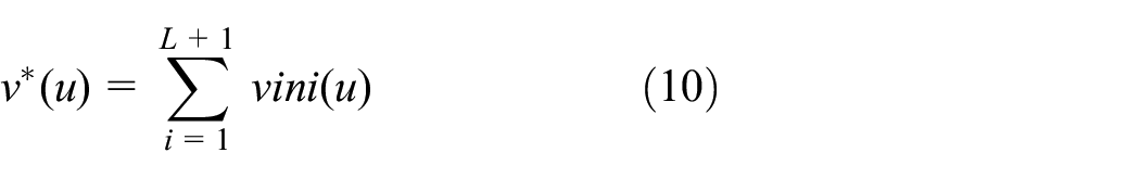
Specifically, a trial function ni(u ) is nonzero only in the interval $u_{i - 1} < u < u_{i + 1}$

n_{i} (u) = \frac{u - u_{i - 1}}{ui - u_{i - 1}} u_{i - 1} \leq u \leq u_{i}

(11)

n_{i} (u) = \frac{u_{i + 1} - u}{u_{i + 1} - u_{i}} u_{i} \leq u \leq u_{i + 1}

(12)

n_{i} (u) = 0 u < u_{i - 1} u > u_{i + 1}

(13)

The trial functions are simply linear interpolation functions approximate solution as given

v * (u) = v_{2} n_{2} (u) + v_{3} n_{3} (u) = v_{2} \frac{u_{3} - u}{u_{3} - u_{2}} + v_{3} \frac{u - u_{2}}{u_{3} - u_{2}}

(14)

Substitution of the assumed solution into the governing equation yields the residual

R (u; v_{i}) = \sum_{i = 1}^{L + 1} [\frac{d^{2} v^{*}}{d u^{2}} + f (u)] = \sum_{i = 1}^{L + 1} [\frac{d^{2}}{d u^{2}} {v_{i} n_{i} (u) + f (u)]

(15)

to which we apply Galerkin’s weighted residual method, using each trial function as a weighting function, to obtain

\begin{matrix} \int_{u_{x}}^{u_{y}} n_{j} (u) R (u; vi) du = \int_{u_{x}}^{u_{y}} n_{j} (u) \sum_{i = 1}^{L + 1} [\frac{d^{2}}{d u^{2}} {v_{i} n_{i} (u) + f (u)] \\ j = 1, M + 1 \end{matrix}

(16)

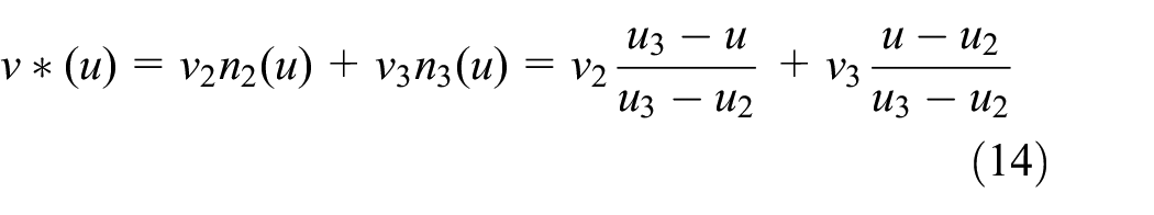
only two of the trial functions are nonzero. Taking this observation into account, now

\int_{u_{j}}^{u_{j + 1}} n_{j} (u) [\frac{d^{2}}{d u^{2}} (v_{j} n_{j} (u) + v_{j + 1} n_{j + 1} (u)) + f (u)] du = 0 j = 1, L + 1

(17)

Integration of equation 34 yields L + 1 algebraic equations in the L + 1 unknown nodal solution values vj, and these equations can be written in the matrix form

[K] {V} = {F}

(18)

where [K] is the system “stiffness” matrix, v is the vector of nodal “displacements” and F is the vector of nodal “forces.”

Application of the numerical solver

During this research, the system of partial differential equations are solved with the aid of finite element method. The resulting variable values are analyzed with the aid of artificial neural network time series analysis.

For many synthetic polymers the glass transition temperature (Tg) is an important parameter. Polymeric materials are in a soft and rubbery condition above Tg. Polymers are in a glassy state below the Tg. This change leads to a growth, free volume, and strength of macro-molecules. Then adding the plasticizers under isothermal conditions has the same results as growth in temperature on molecular strength. The most common method to make petrochemical origin plastics is extrusion. By reducing the temperature the presence of glycerol has a significant plasticizing effect on gluten. One mole of glycerol has the same effect on the depression of wheat gluten Tg.¹⁰

Dynamical properties in hydrogen are found by doing classical equilibrium molecular dynamics (MD) simulations. MD simulations were performed to find the classical energetic and dynamical properties in pure-hydrogen and mixed hydrates at 30 and 200 K. The lightly-filled mixed H2-THF system, in which there is single H2 occupation of the small cage, its found that the largest contribution to the interaction energy of both types of guest is the van der Waals component with the surrounding water molecules. Gas hydrates are crystalline inclusion compounds with a H₂O lattice that makes a periodic array of cages with each cage large enough to contain a gas molecule.¹¹

Air gauges are used as length measuring devices. They have uses in Mechanical Engineering, like in the process control. The main benefits of air gauges are the chances of non-contact measurement, high accuracy, and high sensitivity to the influence of external conditions with vast variety of different measuring applications. Dynamic variables are time and space-dependent in both their magnitude and frequency content. The time constant of the pneumatic system could be reduced down to many milliseconds. The dynamical properties of the air gauge not only depend on the flow-through geometry and the volume of the measuring chamber. It also depends on the pressurized air feeding system and its length and on the outer diameter of the measuring nozzle. Because of its large impact on the static characteristics as well the last parameter cannot be ignored.¹²

ANN time series forecasting tool

The neural network time series helps to forecast the future values with the help of the past values. An approach of tapped delay is used. It is a dynamic approach that works with the aid of tapped delay lines for nonlinear filtering. Data extracted from Comsol Multiphysics was divided into three parts. 70% was used for training, 15% was used for validation and remaining 15% was used for the testing of the model.

Next, to define a nonlinear autoregressive neural network, we have considered 12 hidden layers and two delays. The schematic of the ANN architecture is shown in Figure 7.

Thus with the aid of the time series forecasting, the values for the key variables were depicted in 3D for longer time spans.

Results

Following flow dynamics have been studied during this research:

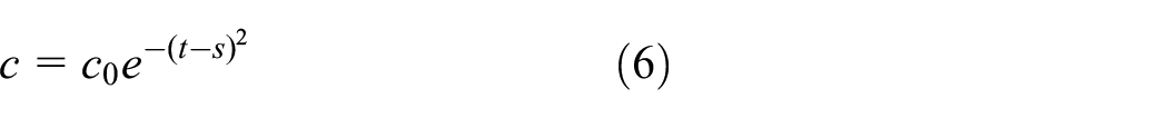
Concentration

Concentration Gradient(c)

Diffusive Flux

Convective Flux

Total Flux

$κ - ε$ 3D model

The 2D model is extended to three dimension, by taking into account the height (h). The 3D model depicts the resulting integral of the outlet concentration as a function of time, and it shows that the residence time is greater than that in the 2D approximation. At slice and streamline, the velocity field has been taken into account. A maximum time was taken of 500 s was achieved with the aid of the ANN forecasting, which is quite greater then 2D model in which maximum time was 200 s.

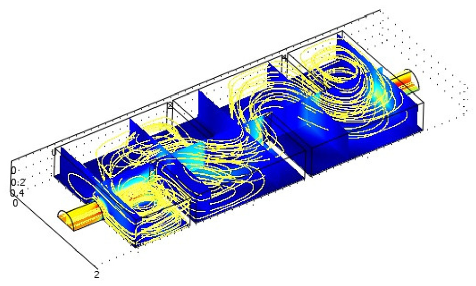
In Figure 8, the three dimensional turbulent reactor is presented. The velocity field and the streamlines are presented in Figure 9. These results were obtained with the aid of step-wise application of FEM and ANN. The dynamics varied relative to different fluid properties as shown in Figures 1, 10 and 11.

Figure 1.

3D reactor of air at time 500 s.

For all the fluids that is, glycerol, air, water, and hydrogen, we have simulated the flow dynamics. The maximum and minimum were depicted for every fluid at different times with a standard step size. The dynamics revealed that the 3D simulations are more realistic since the flow regimens are better visible. The threshold values can also be understood with the aid of the color bars.

Maximum time in 3D model using numerical solver is 200 s, the results were forecasted using ANN and the maximum time of 500 s was achieved.

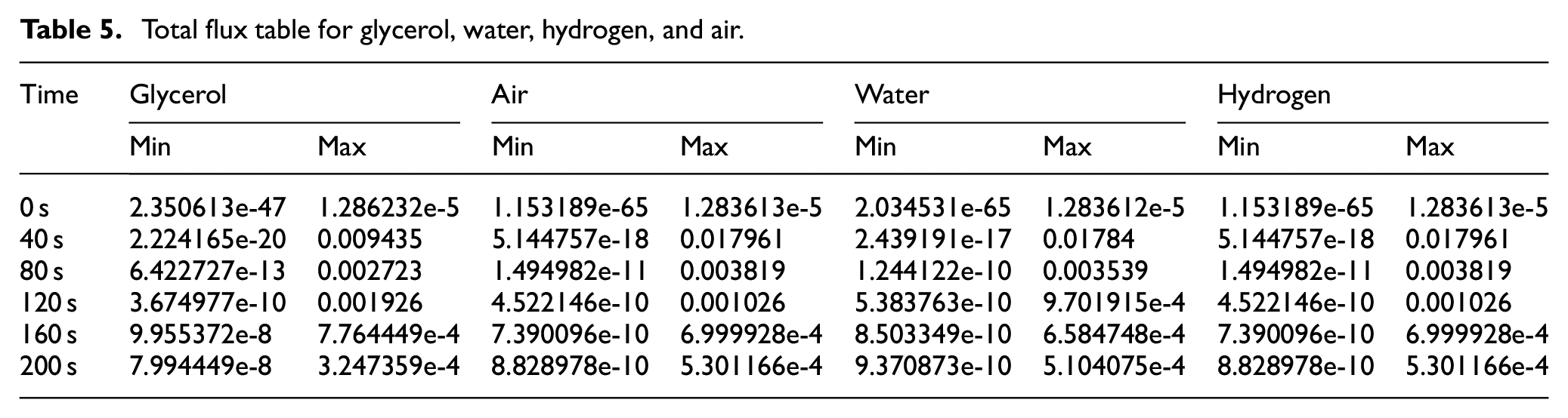
The numerical results obtained are documented in detail with the aid of Tables 1 to 6, and Figures 2 to 11. The video graphic footage for each fluid provides the useful conclusions are enumerated below.

Table 2.

Concentration(c) table for glycerol, water, hydrogen, and air.

Time	Glycerol		Air		Water		Hydrogen
Time	Min	Max	Min	Max	Min	Max	Min	Max
0 s	−2.940779e-5	1.234098e-4	−2.931267e-5	1.234098e-4	−1.11348e-59	1.234098e-4	−2.931272e-5	1.234098e-4
40 s	0.038121	0.115245	−0.042616	0.120162	−0.038453	0.118312	−0.042787	0.12023
80 s	3.879982e-4	0.029783	−1.808451e-5	0.024016	−1.750209e-6	0.023947	−1.784014e-5	0.024025
120 s	−2.649278e-4	0.016678	−5.121119e-5	0.012349	−1.068661e-5	0.011807	−5.147928e-5	0.012342
160 s	−2.152045e-4	0.010571	7.64574e-5	0.009359	−3.518699e-5	0.008993	−7.559631e-5	0.009352
200 s	−2.494794e-4	0.007224	−4.863658e-5	0.007786	−4.586238e-5	0.007787	−4.903301e-5	0.007784

Table 3.

Concentration gradient(c) table for glycerol, water, hydrogen, and air.

Time	Glycerol		Air		Water		Hydrogen
Time	Min	Max	Min	Max	Min	Max	Min	Max
0 s	2.834634e-44	0.003791	1.518772e-63	0.003891	1.140491e-62	0.003891	1.59546e-63	0.003891
40 s	1.342551e-16	0.785638	4.942195e-15	1.467731	4.3041e-14	1.462118	4.828722e-15	1.468646
80 s	3.419186e-9	0.202253	7.846923e-8	0.229363	8.304952e-7	0.23044	7.778568e-8	0.229201
120 s	2.034233e-6	0.159107	1.183839e-6	0.17501	5.7326-6	0.182233	1.131301e-6	0.174121
160 s	1.726377e-5	0.14812	6.408684e-6	0.129217	0.126289	9.054317e-6	6.37494e-6	0.130506
200 s	1.564428e-5	0.073574	1.766052e-6	0.246953	9.978052e-6	0.243046	1.741475e-6	0.249592

Table 4.

Diffusive flux ( $m^{2} / s$ ) table for glycerol, water, hydrogen, and air.

Time	Glycerol		Air		Water		Hydrogen
Time	Min	Max	Min	Max	Min	Max	Min	Max
0 s	4.013449e-47	5.21435e-7	1.815745e-66	4.952384e-7	1.090371e-65	4.952358e-7	1.907832e-66	4.952388e-7
40 s	4.778419e-20	7.209184e-4	3.249574e-18	0.001196	2.257239e-17	0.001185	3.304776e-18	0.001198
80 s	6.653279e-13	1.3866896e-4	7.076763e-12	1.34806e-4	7.542361e-11	1.3355331e-4	7.015138e-12	1.349508e-4
120 s	3.828379e-10	5.862924e-5	1.059697e-10	6.936338e-5	5.383763e-10	7.161273e-5	1.011998e-10	6.907632e-5
160 s	1.674414e-8	5.814157e-5	5.982316e-10	3.422237e-5	8.503349e-10	3.460396e-5	5.950813e-10	3.417331e-5
200 s	2.761847e-9	3.315986e-5	1.5939497e-10	5.589308e-5	9.370873e-10	5.448476e-5	1.571325e-10	5.604222e-5

Table 5.

Total flux table for glycerol, water, hydrogen, and air.

Time	Glycerol		Air		Water		Hydrogen
Time	Min	Max	Min	Max	Min	Max	Min	Max
0 s	2.350613e-47	1.286232e-5	1.153189e-65	1.283613e-5	2.034531e-65	1.283612e-5	1.153189e-65	1.283613e-5
40 s	2.224165e-20	0.009435	5.144757e-18	0.017961	2.439191e-17	0.01784	5.144757e-18	0.017961
80 s	6.422727e-13	0.002723	1.494982e-11	0.003819	1.244122e-10	0.003539	1.494982e-11	0.003819
120 s	3.674977e-10	0.001926	4.522146e-10	0.001026	5.383763e-10	9.701915e-4	4.522146e-10	0.001026
160 s	9.955372e-8	7.764449e-4	7.390096e-10	6.999928e-4	8.503349e-10	6.584748e-4	7.390096e-10	6.999928e-4
200 s	7.994449e-8	3.247359e-4	8.828978e-10	5.301166e-4	9.370873e-10	5.104075e-4	8.828978e-10	5.301166e-4

Table 6.

Convective flux table for glycerol, water, hydrogen, and air.

Time	Glycerol		Air		Water		Hydrogen
Time	Min	Max	Min	Max	Min	Max	Min	Max
0 s	0	1.234089e-5	0	1.234089e-5	0	1.234089e-5	0	1.234089e-5
40 s	0	0.009514	0	0.018017	0	0.017941	0	0.018029
80 s	0	0.00727	0	0.003814	0	0.003538	0	0.003819
120 s	0	0.001927	0	0.001025	0	9.681481e-4	0	0.001024
160 s	0	7.776649e-4	0	6.957939e-4	0	6.580926e-4	0	6.966062e-4
200 s	0	3.244453e-4	0	5.296811e-4	0	5.10289e-4	0	5.298595e-4

Figure 2.

The basic structure of a neuron.

Figure 3.

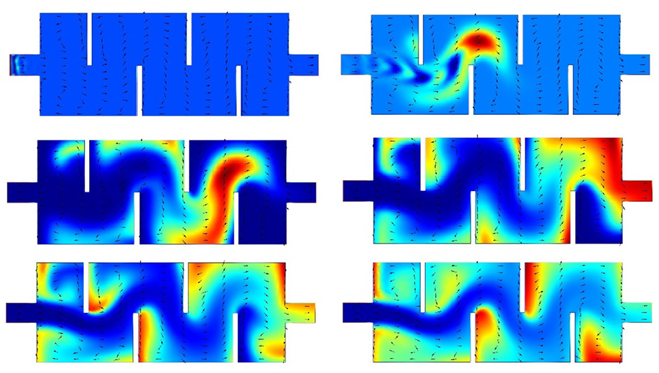
Concentration of glycerol at times t = 0 s,40 s,80 s, 120 s,160 s, and 200 s.

Figure 4.

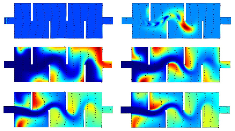
Concentration of water at times t = 0 s,40 s,80 s, 120 s,160 s, and 200 s.

Figure 5.

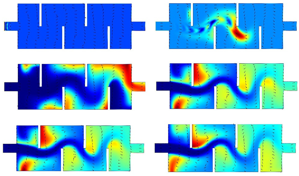
Concentration of hydrogen at times t = 0 s,40 s,80 s, 120 s,160 s, and 200 s.

Figure 6.

Concentration of air at times t = 0 s,40 s,80 s,120 s, 160 s, and 200 s.

Figure 7.

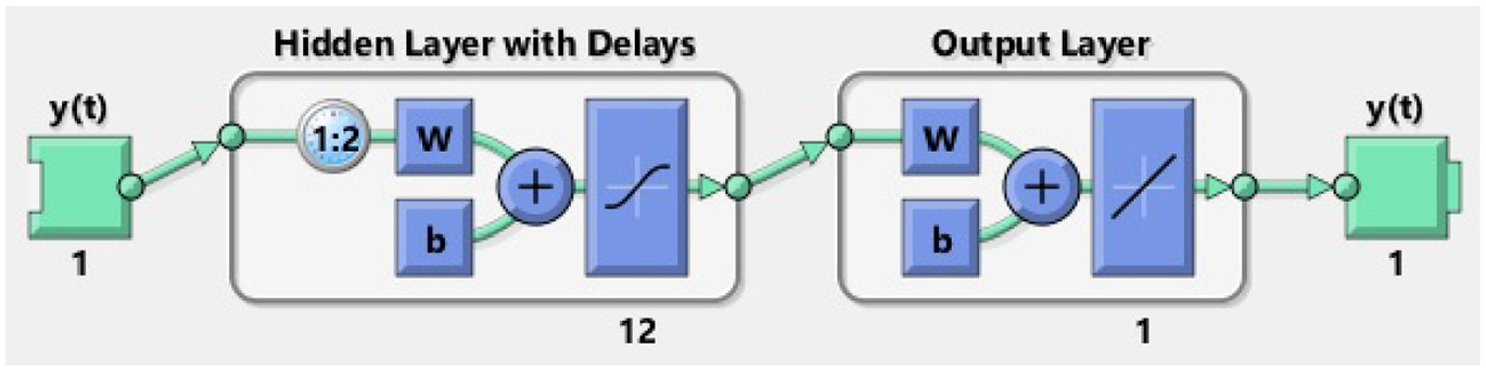
Architecture of ANN for forecasting.

Figure 8.

3D reactor geometry.

Figure 9.

Velocity field and streamlines in the 3D reactor at tie 500 s.

Figure 10.

3D reactor of water at time 500 s.

Figure 11.

3D reactor of hydrogen at time 500 s.

Discussion

During this research, we conclude that specific deviations can be depicted in the dynamics of turbulent $κ - ε$ model.

Initially, to validate the model, we take different fluids including water, hydrogen, glycerol, and air.

We change the dynamics for the water, glycerol, air, and hydrogen model at different times.

Maximum time is 200 s for 2D reactor. It is observed that different changes are shown at different times.

We change the dynamics at sub-domain marker for air, water, glycerol, and hydrogen like concentration gradient, convective flux, and diffusive flux.

Visible changes are observed, when the fluid enters the inlet region at time zero we can see concentration at that starting point.

Furthermore, the transition in time causes dilution throughout the model.

At time 200 s that it is diluted in the model.

We also make 3D models for air, water, and hydrogen, for longer times with the help of ANN.

The work conducted during this research, utilized modern programming tools including the ANN time series forecasting, which can be further extended to formulate better dynamical models at the industrial level for the monitoring of turbulent flows.

Thus glycerol shows the most turbulent dynamics in turbulent reactor.

Conclusion

The proposed model can simulate the viscous fluids efficiently, and it can depict the turbulence to better accuracy. Among all the four fluids, glycerol dynamics were most challenging to depict and higher level of turbulence was observed.

The research strategy documented in this manuscript can prove to be helpful in the field of physics and other engineering and manufacturing fields, where turbulence is the main obstacle in the way of lengthy simulations.

Footnotes

Acknowledgements

This work is supported by the tank engine project: PSF- HIT -085.

Handling Editor: James Baldwin

Declaration of conflicting interests

The author(s) declared no potential conflicts of interest with respect to the research, authorship, and/or publication of this article.

Funding

The author(s) received no financial support for the research, authorship, and/or publication of this article.

ORCID iD

Ayesha Sohail

References

Sheikholeslami

Ganji

. Heat transfer of Cu-water nanofluid flow between parallel plates. Powder Technol 2013; 235: 873–879.

Sheikholeslami

Farshad

. Nanoparticle transportation inside a tube with quad-channel tapes involving solar radiation. Powder Technol 2020; 378: 145–159.

Speziale

Mhuiris

. On the prediction of equilibrium states in homogeneous turbulence. J Fluid Mech 1988; 209: 591.

Khan

Sohail

Sultan

. Effect of anisotropic slip and magnetic field on the flow and heat transfer of Eyring-Powell fluid over an infinite rotating disk. Int J Fluid Mech Res 2017; 44: 257–273.

Sohail

Maqbool

Akbar

, et al. Advanced study of unsteady heat and chemical reaction with ramped wall and slip effect on a viscous fluid. Commun Theor Phys 2017; 67: 301.

Gao

Partohaghighi

Baskonus

, et al. Regarding the group preserving scheme and method of line to the numerical simulations of Klein–Gordon model. Results Phys 2019; 15: 102555.

Essajai

Idrissi

Mortadi

, et al. Numerical based study on charge density wave dynamics in a one-dimensional conductor in the low temperature limit. Results Phys 2019; 12: 1666–1669.

Siddiqui

Sohail

Maqbool

. Analysis of a channel and tube flow induced by cilia. Appl Math Comput 2017; 309: 133–141.

Sherin

Sohail

Shujaat

, et al. Investigation of catalytic potential and radical scavenging efficacy of Terminalia bellerica Roxb Bark mediated ecofriendly silver nanoparticles. J Cluster Sci. Epub ahead of print 29 August 2020. DOI: 10.1007/s10876-020-01865-w.

10.

Pouplin

Redl

Gontard

. Glass transition of wheat gluten plasticized with water, glycerol, or sorbitol. J Agric Food Chem 1999; 47: 538–543.

11.

Gorman

English

MacElroy

. Dynamical and energetic properties of hydrogen and hydrogen–tetrahydrofuran clathrate hydrates. Phys Chem Chem Phys 2011; 13: 19780–19787.

12.

Rucki

Barisic

. Response time of air gauges with different volumes of the measuring chambers. Metrol Meas Syst 2009; 16: 289–298.

Neural network forecasting of the flow regimens of viscous fluids in a 3D reactor

Abstract

Keywords

Introduction

Materials and methods

Materials

Methods

Background of the numerical approach

Numerical Algorithm

The Galerkin finite element method

Application of the numerical solver

ANN time series forecasting tool

Results

κ − ε 3D model

Discussion

Conclusion

Footnotes

Acknowledgements

Declaration of conflicting interests

Funding

ORCID iD

References

$κ - ε$ 3D model