Sage Journals: Discover world-class research

Abstract

Structures dynamic characteristics and their responses can change due to variations in system parameters. With modal characteristics of the structures, their dynamic responses can be identified. Mode shape remains vital in dynamic analysis of the structures. It can be utilized in failure analysis, and the dynamic interaction between structures and their supports to circumvent abrupt failure. Conversely, unlike empty pipes, the mode shapes for pipes conveying fluid are tough to obtain due to the intricacy of the eigenvectors. Unfortunately, fluid pipes can be found in practice in various engineering applications. Thus, due to their global functions, their dynamic and failure analyses are necessary for monitoring their reliability to avert catastrophic failures. In this work, three techniques for obtaining approximate mode shapes (AMSs) of composite pipes conveying fluid, their transition velocity and relevance in failure analysis were investigated. Hamilton’s principle was employed to model the pipe and discretized using the wavelet-based finite element method. The complex modal characteristics of the composite pipe conveying fluid were obtained by solving the generalized eigenvalue problem and the mode shapes needed for failure analysis were computed. The proposed methods were validated, applied to failure analysis, and some vital results were presented to highlight their effectiveness.

Keywords

Composite pipe conveying fluid mode shapes complex eigenvectors wavelets failure

Introduction

Indeed, the involvement of pipes for conveying fluid is increasing on a daily basis and there is no sign that the trend will cease or decline in the nearest future. This is due to the frequent use of pipes for conveying fluid in oil and water pipelines, marine risers, chemical plants, nuclear industry, aerospace, irrigation, and municipality just to mention a few. These pipes are subjected to flow-induced vibration during the operation as a result of turbulence in the flow and this may easily cause pipe failures. Thus, dynamic analysis of the pipes conveying fluid is necessary for monitoring the pipes integrity to avoid failure. Many investigators have worked on pipe failure analysis using different techniques. Bhardwaj et al.¹ examined the reliability of the structure of a pipe-in-pipe in deep-waters under critical operating conditions. In their study, the First-Order and Second-Order, reliability techniques, and Monte Carlo Simulation methods were employed. Chu et al.² analyzed the failure of a steam pipe that has been in service for more than one decade. Finite element analysis and experimental methods were considered during the analysis. Majid et al.³ carried out the failure analysis of eroded pipe using the computational fluid dynamics and experimental methods. Some researchers have also made use of machine learning and dynamic analysis in the pipe failures analysis. For instance, Tang et al.⁴ investigated the plastic water pipe failure using Bayesian network models in which a guided method and automated learning algorithms were employed. Also, Robles-Velasco et al.⁵ employed support vector classification and logistic regression as predictive systems to predict water pipe failures. Ashrafizadeh et al.⁶ studied the crack failure of a gas pipe that has been in service for roughly three decades. In their investigation, dynamic analysis, first mode shape, and others were considered. El-Gebeily et al.⁷ developed a method for detecting pipe internal damage in which vibration modal characteristics were employed and B-spline scaling function was used to formulate the model. Other investigations that have been carried out on pipes failure analysis can be found in Ying et al.,⁸ Rezaei et al.⁹

It can be observed in the above review that pipe mode shapes have not been given much attention in the failure analysis. However, with proper monitoring of the pipe system, any pipe that has been compromised due to internal damage, erosion or chemical attack, and other factors can be detected through the mode shapes. Since geometry can affect mode shapes, monitoring mode shapes can be employed to avoid failure due to the fact that a compromised pipe will display abnormal mode shapes. As a result the majority if not all the failure types or modes observed or mentioned in the review may be avoided. Nevertheless, unlike empty pipes, dynamic analysis of the fluid pipes is difficult because the undamped pipe will become damped as fluid starts flowing through it. Consequently, complex eigenvalues and eigenvectors will emerge and mode shapes constructions become complicated. A suitable technique needs to be employed to be able to obtain mode shapes that can be used in failure analysis, damage assessment, shape estimation, and in order to avoid pessimistic effects of vibration. While significant attentions have been given to the techniques that can be employed to obtain mode shapes of other structures,^10–16 few researchers have paid attentions to the methods for obtaining the mode shapes of pipes conveying fluid. Liu et al.¹⁷ utilized frequency response function based technique to compute mode shapes of fluid pipe while natural frequencies were obtained using a hybrid analytical numerical technique based on the Transfer Matrix Method. Yun-dong and Yi-ren¹⁸ investigated the free vibration analysis of a pipe conveying fluid with different boundary conditions using He’s variational iteration technique and the real part of complex modes was employed to obtain mode shapes. Mediano-Valiente and Garcia Planas¹⁹ studied the dynamics and stability of clamped-pinned pipes conveying fluid using eigenvalues of a Hamiltonian linear system and the natural frequencies and mode shapes employed in their study were also obtained using ANSYS. Arjmandi and Lotfi²⁰ obtained the mode shapes of fluid-structure systems using an accelerated pseudo symmetric subspace iteration method in conjunction with finite element program developed for dynamic analysis of systems. Ryu et al.²¹ employed the concept of quasi-mode shape to examine unstable modal shapes associated with flutter of viscoelastic cantilevered pipes conveying fluid wherein extended Hamilton’s principle was used to obtain equation of motion. Wang et al.²² investigated the mode shapes of cantilevered pipes conveying fluid at different flow velocity in which equation of motion was solved using Differential Quadrature Method. Zhou et al.²³ studied the mode shapes of axially functionally graded cantilevered pipes conveying fluid. Their governing equations and the equations for boundary conditions were also discretized using Differential Quadrature Method. Sarkar and Paidoussis²⁴ utilized semi-analytical approach to obtain the proper orthogonal modes of non-linear oscillation of a cantilevered pipe with end-mass conveying fluid.

Regarding marine risers used widely for conveying fluid, Alfosail et al.²⁵ have obtained the natural frequencies and mode shapes of a marine riser using Galerkin approach in which Euler-Bernoulli beam theory was employed to model the riser. Chen et al.²⁶ utilized differential transformation method to study natural frequencies and mode shapes of marine risers with different boundary conditions.

From the review, one can infer that more needs to be done on the construction of mode shapes of structures or pipes conveying fluid in order to be able to use them to examine the integrity of the pipes regularly to avoid plant down time, revenue loss, and catastrophic failure. The work presented in Oke et al.²⁷ was expanded in this study, more AMSs were presented for different pipes at different velocities, and these mode shapes were used to investigate fluid pipe failure analysis. Hamilton’s principle was utilized to obtain the equation of motion of the composite pipe conveying fluid. The equation was discretized using the wavelet-based finite element method in which Euler-Bernoulli beam theory was employed. The equation obtained was then expressed in state space to obtain the generalized eigenvalue problem. The AMSs used for failure analysis were then constructed from the complex modal characteristics obtained for composite pipe conveying fluid by solving the generalized eigenvalue problem.

Composite pipe conveying fluid system formulation

As the fluid flows through the pipe (see Figure 1) with inlet velocity $v_{1}$ and outlet velocity $v_{2}$ , the fluid pipe interaction will affect the system vibrational behavior and may lead to failure. The strain energy $U$ of the laminated composite pipe element conveying fluid and the total kinetic energy $T$ (which is the summation of kinetic energy of the composite pipe element and the kinetic energy of the fluid element) can be expressed as

U = \frac{1}{2} \int_{0}^{l_{e}} H (x) {(\frac{\partial^{2} y}{\partial x^{2}})}^{2} dx,

(1)

T = \frac{1}{2} \int_{0}^{l_{e}} M (x) V_{p}^{2} dx + \frac{1}{2} \int_{0}^{l_{e}} m_{f} V_{f}^{2} dx,

(2)

where

M (x) = \int \int_{A_{p}} ρ_{p} d A_{p} = \sum_{ℓ = 1}^{N} π ρ_{ℓ} (r_{ℓ}^{2} - r_{ℓ - 1}^{2}) kg / m,

\begin{matrix} V_{f} = (\partial y / \partial t) + V \partial y / \partial x, V_{p} = \partial y / \partial t, \\ A_{p} = 0.25 π (D_{o}^{2} - D_{i}^{2}), A_{f} = 0.25 π D_{i}^{2}, m_{f} = ρ_{f} A_{f}, \end{matrix}

in which $H$ and $M$ are stiffness and mass per unit length of the laminated composite pipe element; $D_{o}$ and $D_{i}$ are pipe outer and inner diameters; and $r_{ℓ}$ and $ρ_{ℓ}$ are radius and density of $ℓ^{th}$ layer. Besides, with stiffness coefficients $A_{11}$ , $B_{11}$ , and $D_{11}$ , an equation utilized in Oke and Khulief²⁸ can be defined for healthy composite pipe conveying fluid shown in Figure 1 as

H = π R^{3} (A_{11} + 2 B_{11} / R + D_{11} / R^{2}),

(3)

where $R = (D_{i} + D_{o}) / 4$ .

Figure 1.

Laminated composite pipe conveying fluid.

Equation of motion of composite pipe conveying fluid

The Hamilton’s principle can be defined as

\int_{t_{1}}^{t_{2}} (δ U - δ T) dt = 0 .

(5)

By substituting equations (1) and (2) in equation (5), it gives

\begin{array}{l} \int_{t_{1}}^{t_{2}} {[\int_{0}^{l_{e}} ℋ (x) \frac{\partial^{4} y}{\partial x^{4}} δ y d x] - [δ (\frac{1}{2} \int_{0}^{l_{e}} m_{e} {(\frac{\partial y}{\partial t})}^{2} d x) \\ + δ (\frac{1}{2} \int_{0}^{l_{e}} 2 m_{f} V \frac{\partial^{2} y}{\partial t \partial x} d x) - \int_{0}^{l_{e}} m_{f} V^{2} \frac{\partial^{2} y}{\partial x^{2}} δ y d x]} d t = 0 . \end{array}

(6)

Then, equation of motion for the laminated composite pipe with fluid flow can be obtained through the simplification of equation (6) as

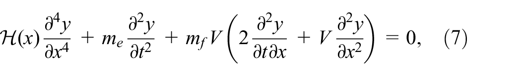
H (x) \frac{\partial^{4} y}{\partial x^{4}} + m_{e} \frac{\partial^{2} y}{\partial t^{2}} + m_{f} V (2 \frac{\partial^{2} y}{\partial t \partial x} + V \frac{\partial^{2} y}{\partial x^{2}}) = 0,

(7)

where $m_{e} = M (x) + m_{f}$ . It should be noted that equation (7) contains four major terms: the pipe stiffness, pipe inertia, Coriolis force, and centrifugal force that arises due to fluid acceleration through the distorted pipe curvature.

The finite element formulation of composite pipe conveying fluid

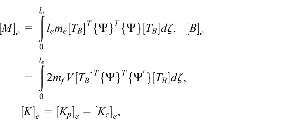
Using the Euler-Bernoulli pipe element, equation (7) has been discretized in order to solve it, wherein theB-spline wavelet on the interval was used as it was in Oke and Khulief.²⁸ As a result, equation (7) can be stated in a condensed form as

[M]_{e} {\begin{matrix} \overset{\cdot\cdot}{y} \end{matrix}}_{e} + [B]_{e} {\begin{matrix} \overset{\cdot}{y} \end{matrix}}_{e} + [K]_{e} {y}_{e} = {0},

(8)

where

\begin{matrix} [M]_{e} = \int_{0}^{l_{e}} l_{e} m_{e} {[T_{B}]}^{T} {Ψ}^{T} {Ψ} [T_{B}] d ζ, [B]_{e} \\ = \int_{0}^{l_{e}} 2 m_{f} V {[T_{B}]}^{T} {Ψ}^{T} {Ψ^{'}} [T_{B}] d ζ, \\ [K]_{e} = [K_{p}]_{e} - [K_{c}]_{e}, \end{matrix}

\begin{matrix} [K_{p}]_{e} = \int_{0}^{l_{e}} \frac{H}{{l_{e}}^{3}} {[T_{B}]}^{T} {Ψ^{″}}^{T} {Ψ^{″}} [T_{B}] d ζ, and [K_{c}]_{e} \\ = \int_{0}^{l_{e}} \frac{1}{l_{e}} m_{f} V^{2} {[T_{B}]}^{T} {Ψ^{'}}^{T} {Ψ^{'}} [T_{B}] d ζ . \end{matrix}

Besides, equation (8) can be stated in state space using the state vectors ${z}$ and ${\begin{matrix} \overset{\cdot}{z} \end{matrix}}$ as

[\bar{M}] {\begin{matrix} \overset{\cdot}{z} \end{matrix}} - [\bar{K}] {z} = {0},

(9)

where

\begin{matrix} [\bar{M}] = [\begin{matrix} [I] & [0] \\ [0] & {[M]}_{e} \end{matrix}], [\bar{K}] = [\begin{matrix} [0] & [I] \\ - {[K]}_{e} & - {[B]}_{e} \end{matrix}], \\ {z} = [\begin{matrix} {y_{1}} \\ {y_{2}} \end{matrix}], {\begin{matrix} \overset{\cdot}{z} \end{matrix}} = [\begin{matrix} \begin{matrix} {{\overset{\cdot}{y}}_{1}} \end{matrix} \\ \begin{matrix} {{\overset{\cdot}{y}}_{2}} \end{matrix} \end{matrix}] . \end{matrix}

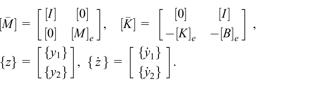
These vectors can be expressed for harmonic motion as

{z} = {W} e^{i ω t}, {\begin{matrix} \overset{\cdot}{z} \end{matrix}} = i ω {W} e^{i ω t} .

(10)

By substituting equation (10) in equation (9), the generalized eigenvalue problem can be obtained as

[[\bar{K}] - λ [\bar{M}]] {W} = {0},

(11)

where $λ = i ω$ and $ω$ is frequency.

Now, the dimension of each matrix in equation (8) is $n \times n$ while that of matrix in equation (11) is $2 n \times 2 n$ .

Numerical results and discussion

Here, AMSs of six pinned-pinned pipes (four composite and two isotropic pipes) were examined and subsequent failure analysis of one of them. The results obtained are as follows:

Composite pipes

The composite pipes ( $P_{1}$ − $P_{2}$ ) defined in Table 1 that have been considered by many investigators along with pipe $P_{3}$ were considered with fluid flow so as to study their vibration behavior and AMSs. Pipe $P_{3}$ uses the stacking sequence given in Bauchau,²⁹ and material and geometric properties of $P_{1}$ except length. In order to validate the model, the fundamental frequency of each pipe without fluid flow was firstly obtained and the results obtained are 98.76, 33.42, and 56.48 Hz respectively. These results agreed with those available in literature or aforementioned Refs. for $P_{1}$ and $P_{2}$ . In addition, the mode shapes for the first four frequencies for these pipes are presented in Figure 2 and it can be seen that they agreed with mode shapes of pinned-pinned structures.

Table 1.

Composite pipes properties.

Property	Pipe $P_{1}$ ^27,30–32	Pipe $P_{2}$ ^28,31,32	Pipe $P_{3}$
$D_{o}$	0.1282 m	0.1126 m	0.1282 m
$D_{i}$	0.1256 m	0.1016 m	0.1256 m
Ply angles/stackingsequence $(^{o})$	[90/45/−45/0₆/90](inner to outer layers)	[±54₅/54](inner to outer layers)	[0/±45/0/45/0/45/0/±45](inner to outer layers)
Length of pipe, L	2.470 m	2.00 m	3.00 m
$E_{11}$	211 $GPa$	12.5 $GPa$	211 $GPa$
$E_{22}$	24.1 $GPa$	7. 1429 $GPa$	24.1 $GPa$
$G_{12} = G_{13} = G_{23}$	6.9 $GPa$	3.3194 $GPa$	6.9 $GPa$
Poisson ratio, $ν_{12}$	0.36	0.56	0.36
Density, $ρ$	1967 $kg / m^{3}$	1730 $kg / m^{3}$	1967 $kg / m^{3}$

Figure 2.

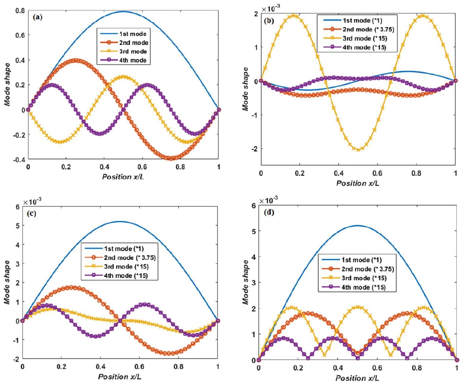
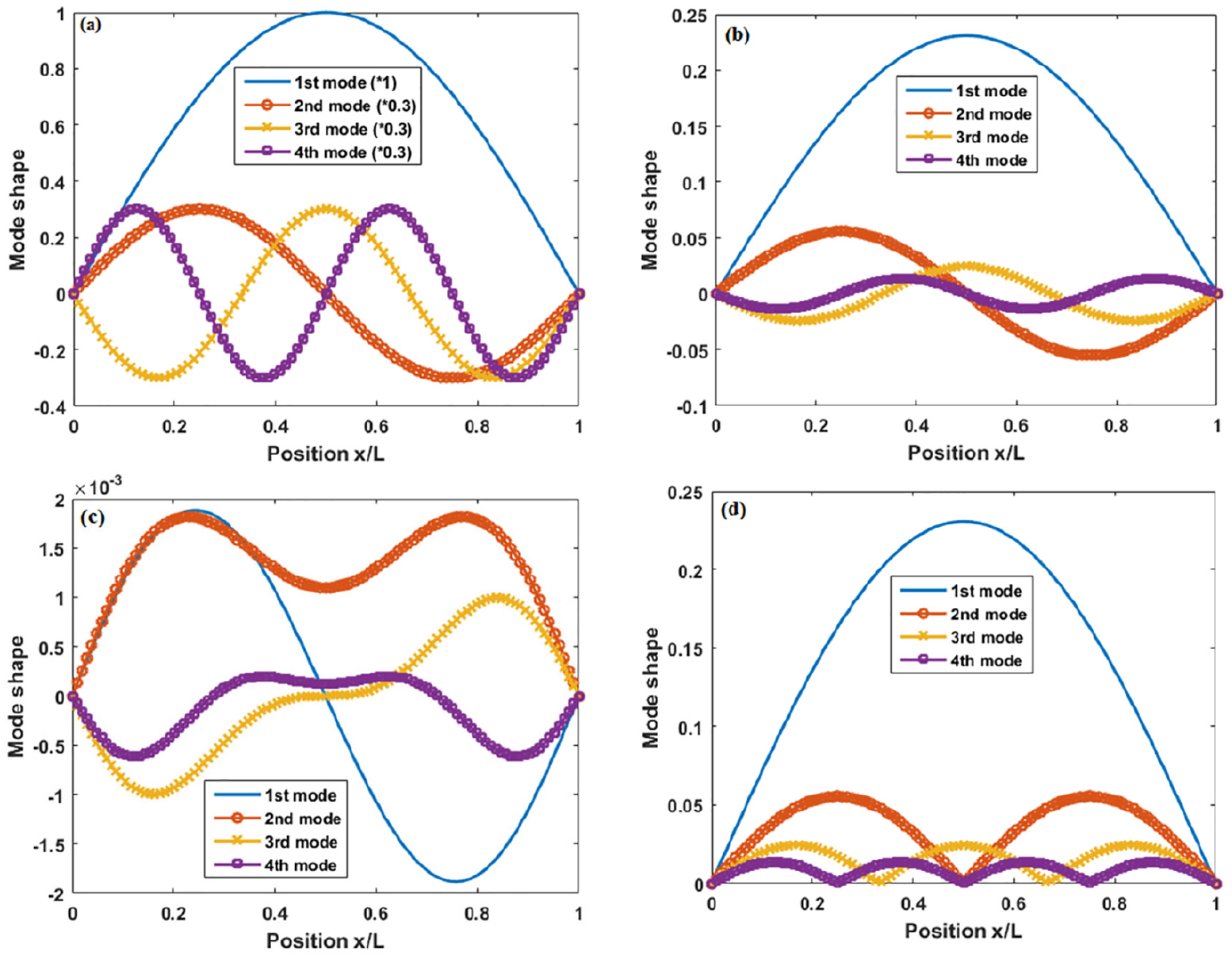
Different pipes mode shapes for the first four frequencies: (a) $P_{1}$ , (b) $P_{2}$ , and (c) $P_{3}$ .

Moreover, each of these pipes was then studied one after the other as the pipe conveying fluid at five different velocities that are less than each pipe critical velocity $V_{c}$ . The fluid used in this investigation was water with density of $998.2 kg / m^{3}$ at all velocities considered. The pipes that were initially undamped suddenly became damped structures as a result of the fluid flowing through them. Consequently, the $2 n$ complex conjugate $λ$ and eigenvectors were obtained but these made the mode shapes to become difficult to obtain as in Figure 2. Nevertheless, by using any of the following three methods: real part, imaginary part, and absolute of complex eigenvectors; the AMSs were obtained from complex eigenvectors. The AMSs obtained for the pipes conveying fluid (damped pipes) at different velocities are compared with their mode shapes (in Figure 2) when they were empty pipes (undamped pipes). The results obtained are as presented in Figures 3 to 7 for $P_{1}$ , Figures 8 to 12 for $P_{2}$ , and Figures 13 to 17 for $P_{3}$ respectively, where “(a)” in Figures 3 to 7 is the same as Figure 2(a), “(a)” in Figures 8 to 12 is the same as Figure 2(b), and “(a)” in Figures 13 to 17 is the same as Figure 2(c). It can be found that the mode shapes for the pipes had been reduced generally when compared to those available when they were empty. Besides, at lower velocities, it is fascinating to see that the mode shapes obtained for these pipes from the imaginary part of their complex eigenvectors offered the mode shapes that are similar to pinned-pinned pipes mode shapes (see Figure 2). At the same time, the absolute of the eigenvectors displayed similar mode shapes in the positive side but the real part of eigenvectors produced wrong mode shapes which cannot be used for further analysis. However, one can observe that as velocity increases, the real part of eigenvectors gives the needed mode shapes, absolute of eigenvectors continues displaying the mode shapes in the positive side while the mode shapes from imaginary part are no longer depict acceptable mode shapes.

Figure 3.

(a) Mode shapes for empty Pipe; (b–d) are imaginary, real, and absolute mode shapes for pipe conveying fluid at V = 10 m/s.

Figure 4.

(a) Mode shapes for empty Pipe; (b–d) are imaginary, real, and absolute mode shapes for pipe conveying fluid at V = 60 m/s.

Figure 5.

(a) Mode shapes for empty Pipe; (b–d) are imaginary, real, and absolute mode shapes for pipe conveying fluid at V = 70 m/s.

Figure 6.

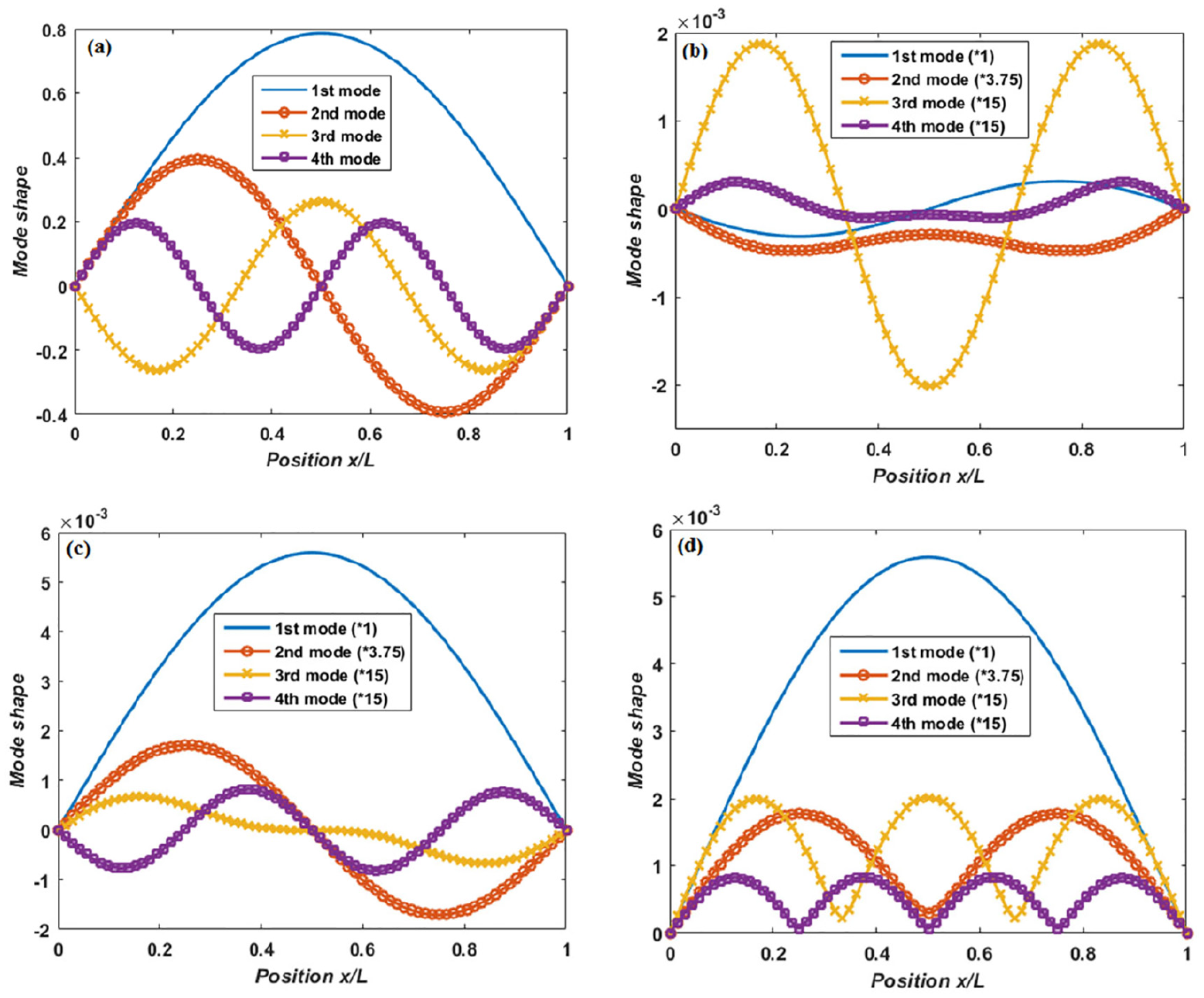
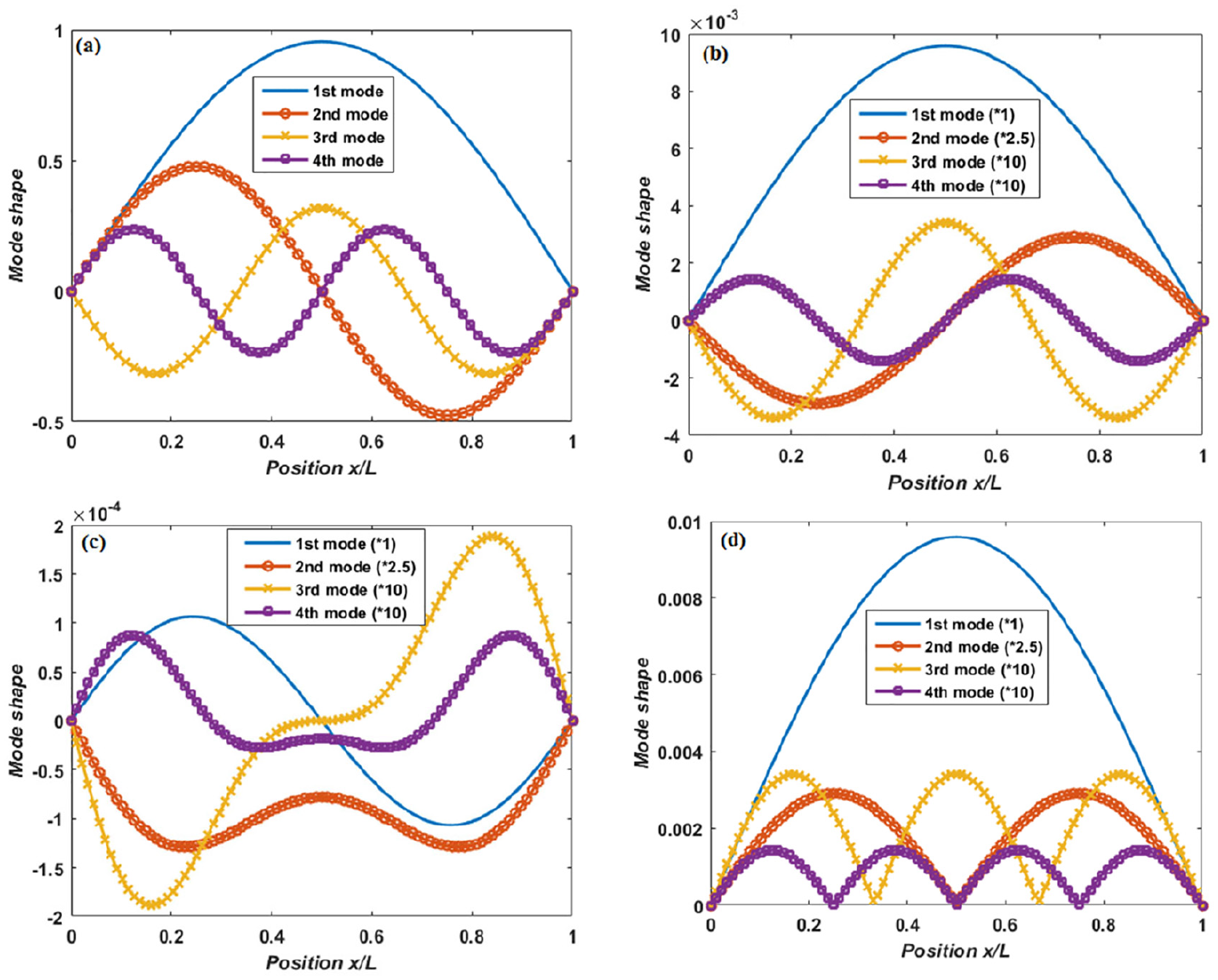
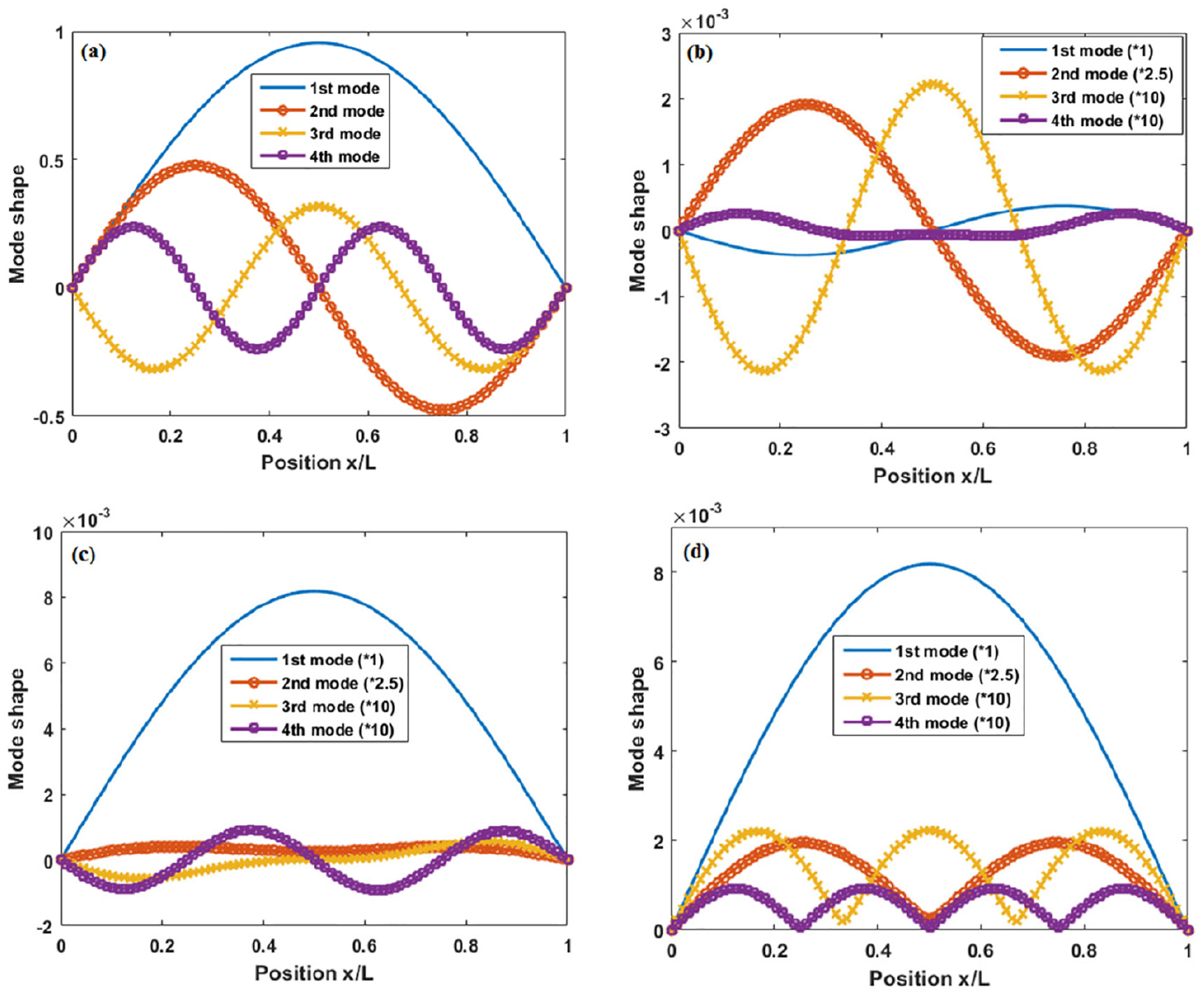
(a) Mode shapes for empty Pipe; (b–d) are imaginary, real, and absolute mode shapes for pipe conveying fluid at V = 80 m/s.

Figure 7.

(a) Mode shapes for empty Pipe; (b–d) are imaginary, real, and absolute mode shapes for pipe conveying fluid at V = 90 m/s.

Figure 8.

(a) Mode shapes for empty Pipe; (b–d) are imaginary, real, and absolute mode shapes for pipe conveying fluid at V = 10 m/s.

Figure 9.

(a) Mode shapes for empty Pipe; (b–d) are imaginary, real, and absolute mode shapes for pipe conveying fluid at V = 40 m/s.

Figure 10.

(a) Mode shapes for empty Pipe; (b–d) are imaginary, real, and absolute mode shapes for pipe conveying fluid at V = 50 m/s.

Figure 11.

(a) Mode shapes for empty Pipe; (b–d) are imaginary, real, and absolute mode shapes for pipe conveying fluid at V = 60 m/s.

Figure 12.

(a) Mode shapes for empty Pipe; (b–d) are imaginary, real, and absolute mode shapes for pipe conveying fluid at V = 70 m/s.

Figure 13.

(a) Mode shapes for empty Pipe; (b–d) are imaginary, real, and absolute mode shapes for pipe conveying fluid at V = 10 m/s.

Figure 14.

(a) Mode shapes for empty Pipe; (b–d) are imaginary, real, and absolute mode shapes for pipe conveying fluid at V = 40 m/s.

Figure 15.

(a) Mode shapes for empty Pipe; (b–d) are imaginary, real, and absolute mode shapes for pipe conveying fluid at V = 50 m/s.

Figure 16.

(a) Mode shapes for empty Pipe; (b–d) are imaginary, real, and absolute mode shapes for pipe conveying fluid at V = 60 m/s.

Figure 17.

(a) Mode shapes for empty Pipe; (b–d) are imaginary, real, and absolute mode shapes for pipe conveying fluid at V = 70 m/s.

Furthermore, it can be observed from these figures that among the three methods examined for obtaining mode shapes from the complex eigenvectors, mode shapes from either absolute or imaginary part of eigenvectors can be used to study fluid pipe displacement, failure, and other analyses at lower velocities. Conversely, at higher velocities, the mode shapes from absolute or real part of eigenvectors can be employed for fluid pipe displacement, failure, and other analyses. It becomes necessary to point out that the mode shapes obtained from absolute eigenvectors that is consistent at any velocity can be modified to look like Figure 2 by changing the signs of the required areas. Thus, instead of employing the mode shapes shown in Figure 2 that are not correct mode shapes for the pipe conveying fluid for failure and further analyses, AMSs obtained from any of these methods can be utilized.

In addition, the very significant observation was observed when acceptable AMSs for $P_{1}$ , $P_{2}$ , and $P_{3}$ abruptly shifted from imaginary part to real part of complex eigenvectors as velocity increases. It was noticed further that around this phenomenon, one or more of acceptable AMSs are presented by imaginary part while the rest are produced by real part of complex eigenvectors. This abrupt shift occurred between velocities of 60–70 m/s (see Figures 4 and 5) for $P_{1}$ , between 40 and 50 m/s (see Figures 9 and 10) for $P_{2}$ , and between 40 and 50 m/s (see Figures 14 and 15) for $P_{3}$ respectively. Further examinations around these velocities revealed that the transition of the acceptable AMSs from imaginary part to real part of complex eigenvectors commenced at velocity greater than 64, 42, and 44 m/s in that order for $P_{1}$ , $P_{2}$ , and $P_{3}$ . Interestingly, velocity of 64 m/s is closer to $V_{h}$ of $P_{1}$ , 42 m/s is closer to $V_{h}$ of $P_{2}$ while 44 m/s is also closer to $V_{h}$ of $P_{3}$ . Where $V_{h}$ is the half of the critical velocity $V_{c}$ and $V_{c}$ is the velocity at which fluid pipe will fracture or fail. The details can be found in Table 2. If this table is looked into critically, it will be observed that the transition velocity $V_{t}$ for each pipe is not far from the half of its $V_{c}$ . The $V_{t}$ is the velocity at which first mode loses shape in the imaginary part of the complex eigenvectors and appears fully in the real part of complex eigenvectors. Although, four modes were considered in this study but $V_{t}$ is related to only first mode because it will occur first among all modes, it is the most destructive mode, and it is also most important in the structural dynamic analysis.

Table 2.

Transition and critical velocities.

Pipe	Transition conditions			Critical conditions
	Velocityrange (m/s)	Velocity $V_{t}$ ^* (m/s)	First frequency(Hz) for $V_{t}$	Velocity range (m/s)	Velocity $V_{c}$ ^* (m/s)	First frequency(Hz) for $V_{c}$
$P_{1}$	64–65	64.53	23.7233	140–141	140.08	0
$P_{2}$	42–43	42.77	15.0382	84–85	84.09	0
$P_{3}$	44–45	44.73	13.5749	97–98	97.30	0

Velocity with two decimal points.

Furthermore, it can also be noticed from these figures that as velocity is closer to the transition velocity, the mode shapes obtained from the imaginary part of complex eigenvectors begin to lose their forms one after the other while reverse was the case regarding the mode shapes obtained from the real part. Hence, different from what was reported in literature, it can be inferred that neither only imaginary part nor only real part of complex eigenvectors is sufficient to obtain acceptable mode shapes of pipes conveying fluid at different velocities.

Further, another pipe $P_{4}$ was utilized to investigate the effect of length on AMSs. This pipe has the same properties as $P_{1}$ but its $D_{i}, D_{o}$ , and $L$ are $0.292, 0.324,$ and $32 m$ respectively. It is first frequency when it was undamped is $1.4112 Hz$ . When this pipe becomes fluid pipe at different velocities, it was observed that mode shapes and $V_{t}$ behaved like those in the previous pipes.

Isotropic pipes

The observations under composite pipes extended this investigation to isotropic pipes and as a result, the model was modified to be able to handle isotropic pipes. The pipes $P_{5}$ and $P_{6}$ considered are defined in Table 3. The modified model was validated with empty $P_{5}$ and $P_{6}$ and the first natural frequency for each pipe was obtained to be 39.6296 and $0.8465 Hz$ . To validate the model further, the first frequency of $P_{6}$ at 0 $m / s$ was determined and the result obtained (0.6955 $Hz$ ) is the same as in Bao-hui et al.³³ This shows the accuracy of the model. The mode shapes for the first four frequencies of these pipes when they were empty are as shown in Figure 18 and it can be observe that they are also agreed with mode shapes of pinned-pinned structures.

Table 3.

Isotropic pipes properties.

Property	Pipe $P_{5}$	Pipe $P_{6}$ ³³
$D_{o}$	0.1282 m	0.324 m
$D_{i}$	0.1256 m	0.292 m
Length of pipe, L	3.00 m	32.00 m
Modulus of elasticity, $E$	210 $GPa$	210 $GPa$
Poisson ratio, $ν$	0.3	0.3
Density, $ρ$	8200 $kg / m^{3}$	8200 $kg / m^{3}$

Figure 18.

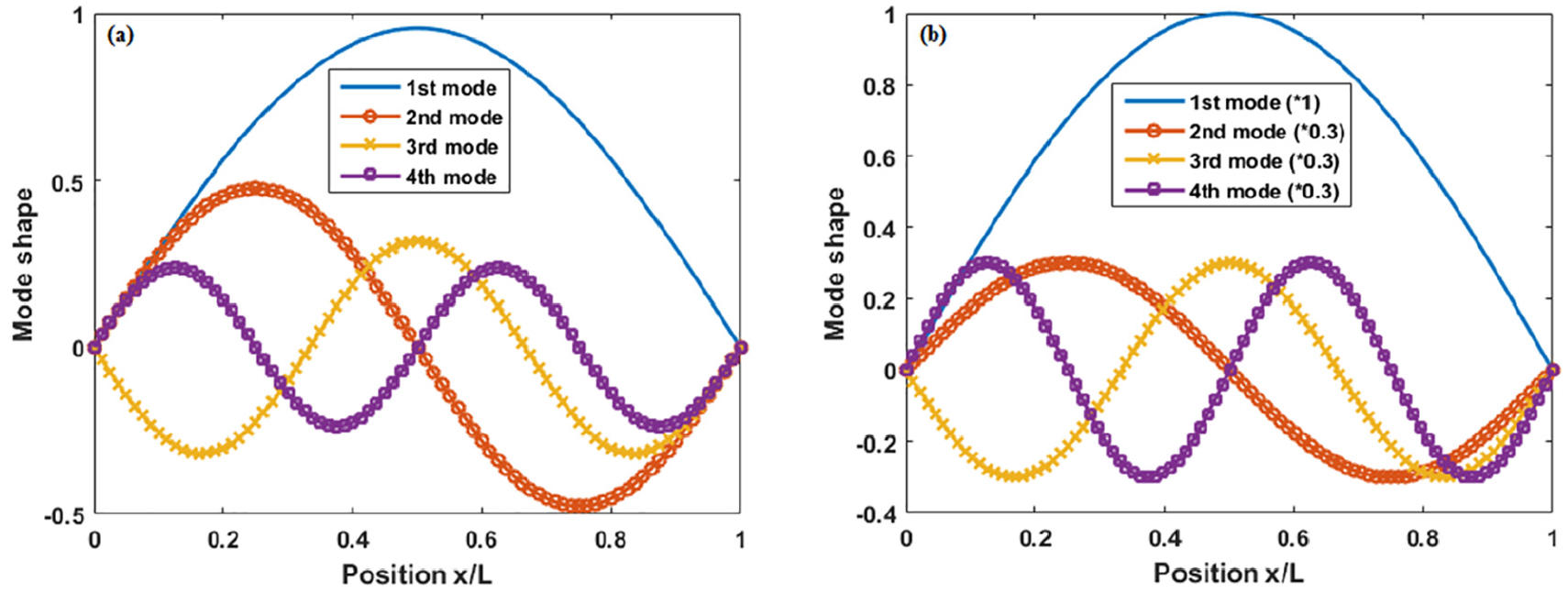
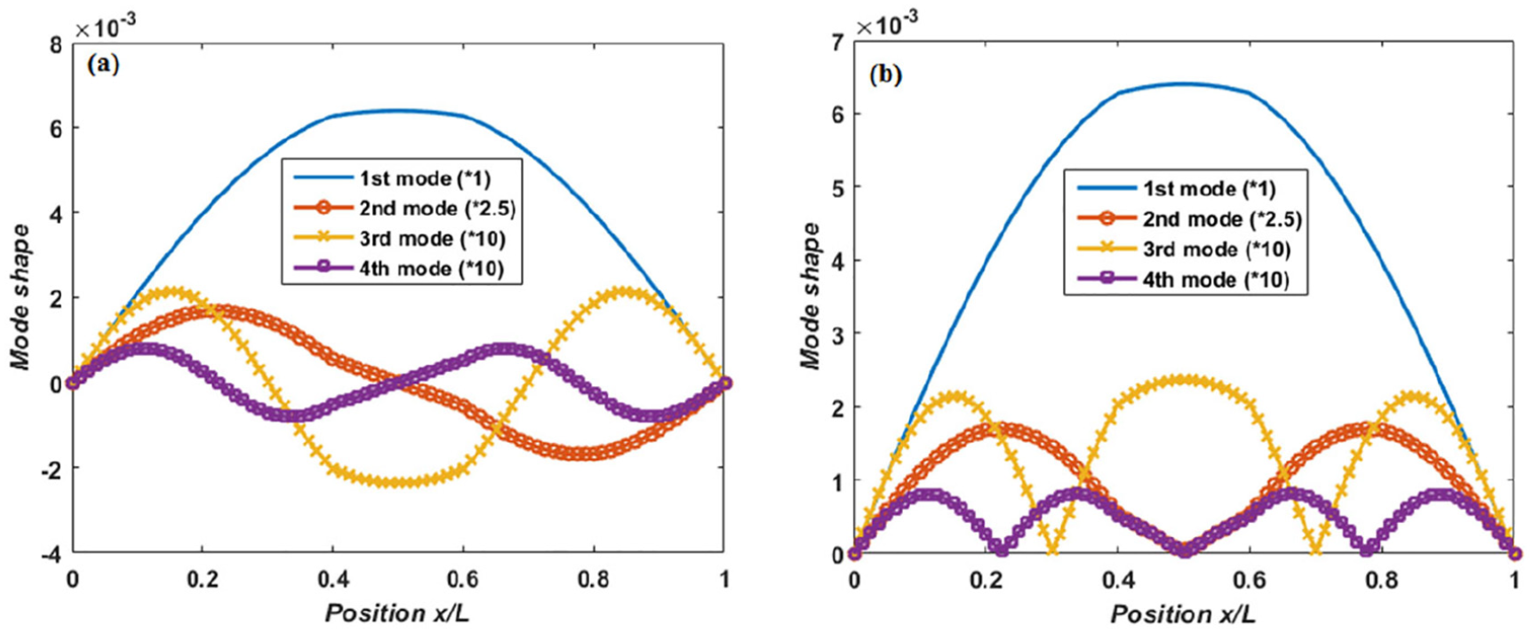
Different pipes mode shapes for the first four frequencies: (a) $P_{5}$ and (b) $P_{6}$ .

Now, as it was done under composite pipes, each of these pipes was then examined one after the other as the pipe conveying fluid at five different velocities that are less than each pipe critical velocity $V_{c}$ . The AMSs obtained for these pipes conveying fluid at different velocities are compared with their mode shapes (in Figure 18) when they were empty pipes. The results obtained are as presented in Figures 19 to 23 for $P_{5}$ , and Figures 24 –28 for $P_{6}$ respectively where “(a)” in Figures 19 to 23 is the same as Figure 18(a) and “(a)” in Figures 24 to 28 is the same as Figure 18(b). The same things observed in figures for composite pipes were also observed in figures for isotropic pipes. The details can be found in Table 4. It will be noticed in this table that the transition velocity $V_{t}$ for $P_{5}$ is not far from its $V_{h}$ as in Table 2 unlike that of $P_{6}$ that is away from $V_{h}$ but it is closer to $V_{h}$ when compare to $V_{c}$ .

Figure 19.

(a) Mode shapes for empty Pipe; (b–d) are imaginary, real, and absolute mode shapes for pipe conveying fluid at V = 10 m/s.

Figure 20.

(a) Mode shapes for empty Pipe; (b–d) are imaginary, real, and absolute mode shapes for pipe conveying fluid at V = 70 m/s.

Figure 21.

(a) Mode shapes for empty Pipe; (b–d) are imaginary, real, and absolute mode shapes for pipe conveying fluid at V = 80 m/s.

Figure 22.

(a) Mode shapes for empty Pipe; (b–d) are imaginary, real, and absolute mode shapes for pipe conveying fluid at V = 90 m/s.

Figure 23.

(a) Mode shapes for empty Pipe; (b–d) are imaginary, real, and absolute mode shapes for pipe conveying fluid at V = 100 m/s.

Figure 24.

(a) Mode shapes for empty Pipe; (b–d) are imaginary, real, and absolute mode shapes for pipe conveying fluid at V = 10 m/s.

Figure 25.

(a) Mode shapes for empty Pipe; (b–d) are imaginary, real, and absolute mode shapes for pipe conveying fluid at V = 50 m/s.

Figure 26.

(a) Mode shapes for empty Pipe; (b–d) are imaginary, real, and absolute mode shapes for pipe conveying fluid at V = 60 m/s.

Figure 27.

(a) Mode shapes for empty Pipe; (b–d) are imaginary, real, and absolute mode shapes for pipe conveying fluid at V = 70 m/s.

Figure 28.

(a) Mode shapes for empty Pipe; (b–d) are imaginary, real, and absolute mode shapes for pipe conveying fluid at V = 78 m/s.

Table 4.

Isotropic pipes transition and critical velocities.

Pipe	Transition conditions			Critical conditions
Pipe	Velocityrange (m/s)	Velocity $V_{t}$ ^* (m/s)	First frequency(Hz) at $V_{t}$	Velocity range (m/s)	Velocity $V_{c}$ ^* (m/s)	First frequency(Hz) at $V_{c}$
$P_{5}$	73–74	73.64	17.5938	146–147	146.20	0
$P_{6}$	50–51	50.24	0.5263	78–79	78.30	0

Velocity with two decimal points.

Moreover, in all the six pipes considered, it was observed that the AMSs needed for pipe failure analysis can be obtained as follows: imaginary part of complex mode shapes will give AMSs at lower fluid velocity, real part of complex mode shapes will give AMSs at higher fluid velocity while both imaginary and real parts are required to obtain AMSs around transition velocities.

Pipes failure analysis

The mode shapes obtained under different pipes are needed for successful failure analysis based on the velocity of the fluid in the pipe under consideration. It should be noted that all the pipes that have been considered above are healthy pipes and AMSs obtained at different velocities depict the actual shapes of such mode shapes. However, these mode shapes will not have the shapes of actual mode shapes once the integrity of any of these pipes (see Figure 29 ) is compromised. The pipe defect can grow in radial or longitudinal direction or both as time passes by. Thus, if the cross-sections of the region with and region without defect in Figure 29 are expanded they can be presented as shown in Figure 30. In this figure, $t_{o}$ , $t_{n}$ , $t_{d}$ , and $l_{d}$ are original pipe thickness, thickness of the region not affected by defect, thickness of defected region, and length of the defect along pipe span respectively. The pipe defect could form any shape but in this work, the defect is assumed to be circular for simplicity as shown in Figure 30(c). The mass and stiffness of the region with defect will continue to change as defect shape increases while the volume of the fluid at the region will increase.

Figure 29.

Pipe with internal defect.

Figure 30.

Cross-sections of different regions of pipe with internal defect: (a) cross-section of region without defect, (b) cross-section of the region with defect, and (c) pipe defect and its width.

As a case study, pipe $P_{2}$ was considered as a pipe with defect wherein $t_{d} = t_{o} / 2 m$ ; $l_{d} = L / 10 m$ ; and $l_{c} = L / 4$ , $L / 2$ , and $4 L / 5 m$ where $l_{c}$ is the defect location along the pipe span. The frequencies of this defected pipe as an empty and as a pipe conveying fluid are presented in Tables 5 and 6 in that order. The effects of the defect on the pipe can be seen in both tables and these will continue as the defect grows till the failure eventually occurs.

Table 5.

Frequency of empty pipe $P_{2}$ with defect at different locations.

S/N	Frequency ofhealthy pipe $P_{2}$ ( $Hz$ )	Frequency of pipe $P_{2}$ with defect ( $Hz$ )
S/N	Frequency ofhealthy pipe $P_{2}$ ( $Hz$ )	$l_{c} = L / 4 m$	$l_{c} = L / 2 m$	$l_{c} = 4 L / 5 m$
1	33.4224	32.9600	32.5790	33.0873
2	133.6896	131.6241	133.5404	131.6785
3	300.8017	299.4132	298.8008	298.6914
4	534.7590	532.8752	532.8749	533.2888
5	835.5622	835.0721	838.5242	831.6705

Table 6.

Frequency of pipe $P_{2}$ conveying fluid with defect at different locations.

Velocity (m/s)	Pipe type		Frequency ( $Hz$ )
			$f_{1}$	$f_{2}$	$f_{3}$	$f_{4}$	$f_{5}$
0	Healthy pipe		17.7944	71.1778	160.1500	284.7113	444.8621
	Pipe with defect	$l_{c} = L / 4 m$	17.1242	66.6366	155.3530	281.9764	430.8833
		$l_{c} = L / 2 m$	16.5461	70.9949	150.9925	281.9795	424.9021
		$l_{c} = 4 L / 5 m$	17.3191	66.8735	152.0967	278.3392	438.5106
10	Healthy pipe		17.6508	71.0684	160.0501	284.6162	444.7698
	Pipe with defect	$l_{c} = L / 4 m$	16.9739	66.5206	155.2505	281.8803	430.7889
		$l_{c} = L / 2 m$	16.3911	70.8842	150.8905	281.8838	424.8072
		$l_{c} = 4 L / 5 m$	17.1709	66.7569	151.9919	278.2423	438.4172
60	Healthy pipe		12.0034	67.1654	156.5336	281.2786	441.5369
	Pipe with defect	$l_{c} = L / 4 m$	10.9959	62.3643	151.6402	278.5070	427.4814
		$l_{c} = L / 2 m$	10.0818	66.9386	147.2962	278.5277	421.4819
		$l_{c} = 4 L / 5 m$	11.3155	62.5753	148.3008	274.8427	435.1400

Furthermore, the presence of the defect in the pipe can be noticed in the pipe mode shapes in which they will be deformed unlike when the pipe is healthy. This deformation will appear around the location where defect is present along the pipe span. Figures 31 to 33 show the new deformed mode shapes of Figure 8(b) and (d) while Figures 34 to 36 display the new deformed mode shapes of Figure 11(b) to (d) for pipe $P_{2}$ when its integrity has been compromised with internal defect as shown in Figure 29. This defect may occur due to erosion, chemical attack or other factors at different locations along the pipe span. Once this occurred, the pipes can be marked for maintenance or replacement to prevent total failure and its consequences.

Figure 31.

(a, b) Imaginary and absolute mode shapes for pipe with internal defect at l_c = L/4 and conveying fluid at V = 10 m/s.

Figure 32.

(a, b) Imaginary and absolute mode shapes for pipe with internal defect at l_c= L/2 and conveying fluid at V = 10 m/s.

Figure 33.

(a, b) Imaginary and absolute mode shapes for pipe with internal defect at l_c= 4L/5 and conveying fluid at V = 10 m/s.

Figure 34.

(a–c) Imaginary, real, and absolute mode shapes for pipe with internal defect at lc=L/4 and conveying fluid at V=60 m/s.

Figure 35.

(a–c) are imaginary, real, and absolute mode shapes for pipe with internal defect at l_c= L/2 and conveying fluid at V = 60 m/s.

Figure 36.

(a–c) Imaginary, real, and absolute mode shapes for pipe with internal defect at l_c= 4L/5 and conveying fluid at V = 60 m/s.

Conclusions

Mode shapes are crucial in dynamic analysis of the structures. Three different techniques for obtaining AMSs of pipes with flowing fluid and their characteristics as the fluid velocity increases were presented, and their application in the pipe failure analysis were investigated in this work. It was observed that when there is substantial compromise in the pipe integrity due to erosion, chemicals in the fluid, corrosion, and so on; the mode shapes will be deformed. The real deformation that will indicate that the pipe has been compromised will appear in one or more of the three methods presented based on the fluid velocity. In this study, at lower velocities this actual deformation was noticed in the mode shapes from imaginary part or absolute of complex eigenvectors while it appeared in the mode shapes from the real part or absolute of complex eigenvectors at higher velocities. On the contrary, the deformation emerged in the mode shapes from all techniques around transition velocities. Once the actual deformation is noticed, the pipe under consideration can be marked as the pipe that will fail sooner or later if necessary maintenance is not done.

Hence, the findings in this study support the initiative that AMSs can be employed to assess or monitor fluid pipe integrity in order to reduce revenue loss, leakage, plant shutdown time, and prevent catastrophic failures.

Footnotes

Handling Editor: Chenhui Liang

Declaration of conflicting interests

The author(s) declared no potential conflicts of interest with respect to the research, authorship, and/or publication of this article.

Funding

The author(s) received no financial support for the research, authorship, and/or publication of this article.

ORCID iD

Wasiu Adeyemi Oke

References

Bhardwaj

Teixeira

Soares

. Reliability assessment of a subsea pipe-in-pipe system for major failure modes. Int J Press Vessel Piping 2020; 188: 104177.

Chu

Zhang

, et al. Failure analysis of a steam pipe weld used in power generation plant. Eng Fail Anal 2014; 44: 363–370.

Majid

Mohsin

Yusof

. Experimental and computational failure analysis of natural gas pipe. Eng Fail Anal 2012; 19: 32–42.

Tang

Parsons

Jude

. Comparison of automatic and guided learning for Bayesian networks to analyse pipe failures in the water distribution system. Reliab Eng Syst Saf 2019; 186: 24–36.

Robles-Velasco

Cortés

Muñuzuri

, et al. Prediction of pipe failures in water supply networks using logistic regression and support vector classification. Reliab Eng Syst Saf 2020; 196: 106754.

Ashrafizadeh

Karimi

Ashrafizadeh

. Failure analysis of a high pressure natural gas pipe under split tee by computer simulations and metallurgical assessment. Eng Fail Anal 2013; 32: 188–201.

El-Gebeily

Khulief

Ghneim

. A multiresolution approach for damage detection in fiber-reinforced polymer pipe systems. Adv Mech Eng 2016; 8: 1687814016668707.

Ying

Cuiyun

Yanhui

. Pipe defect detection and reconstruction based on 3D points acquired by the circular structured light vision. Adv Mech Eng 2013; 5: 670487.

Rezaei

Ryan

Stoianov

. Pipe failure analysis and impact of dynamic hydraulic conditions in water supply networks. Procedia Eng 2015; 119: 253–262.

10.

Zhang

Zhao

Lie

. Estimation of mode shapes of beam-like structures by a moving lumped mass. Eng Struct 2019; 180: 654–668.

11.

. Computer animation of structural mode shapes. In: 2014 international conference on multimedia computing and systems (ICMCS), Marrakech, Morocco, 14–16 April 2014, pp.1–4.

12.

Thomas

Gurusamy

Rajanna

, et al. Structural shape estimation by mode shapes using fiber bragg grating sensors: a genetic algorithm approach. IEEE Sens J 2019; 20: 2945–2952.

13.

Koruk

Sanliturk

. A novel definition for quantification of mode shape complexity. J Sound Vib 2013; 332: 3390–3403.

14.

Zhou

. A novel mode shape reconstruction method for damage diagnosis of cracked beam. Mech Syst Signal Process 2019; 122: 433–447.

15.

El-Sayed

El-Mongy

. Free vibration and stability analysis of a multi-span pipe conveying fluid using exact and variational iteration methods combined with transfer matrix method. Appl Math Model 2019; 71: 173–193.

16.

Bahaadini

Dashtbayazi

Hosseini

, et al. Stability analysis of composite thin-walled pipes conveying fluid. Ocean Eng 2018; 160: 311–323.

17.

Liu

Wang

Zhou

, et al. Vibration response of multi-span fluid-conveying pipe with multiple accessories under complex boundary conditions. Eur J Mech A Solids 2018; 72: 41–56.

18.

Yun-dong

Yi-ren

. Vibration analysis of conveying fluid pipe via He’s variational iteration method. Appl Math Model 2017; 43: 409–420.

19.

Mediano-Valiente

Garcia Planas

. Stability analysis of a clamped-pinned pipeline conveying fluid. WSEAS Trans Syst 2014; 13: 54–64.

20.

Arjmandi

Lotfi

. Computing mode shapes of fluid-structure systems using subspace iteration methods. Sci Iran 2011; 18: 1159–1169.

21.

Ryu

S-U

Sugiyama

Ryu

B-J

. Eigenvalue branches and modes for flutter of cantilevered pipes conveying fluid. Comput Struct 2002; 80: 1231–1241.

22.

Wang

Dai

. Nonconservative pipes conveying fluid: evolution of mode shapes with increasing flow velocity. J Vib Control 2015; 21: 3359–3367.

23.

Zhou

X-W

Dai

H-L

Wang

. Dynamics of axially functionally graded cantilevered pipes conveying fluid. Compos Struct 2018; 190: 112–118.

24.

Sarkar

Paidoussis

. A cantilever conveying fluid: coherent modes versus beam modes. Int J Non Linear Mech 2004; 39: 467–481.

25.

Alfosail

Nayfeh

Younis

. Natural frequencies and mode shapes of statically deformed inclined risers. Int J Non Linear Mech 2017; 94: 12–19.

26.

Chen

Chai

, et al. An extraction of the natural frequencies and mode shapes of marine risers by the method of differential transformation. Comput Struct 2009; 87: 1384–1393.

27.

Oke

Adeyemi

Bello

, et al. Approximate mode shape for damped structures. In: Gdoutos

(ed.) Proceedings of the second international conference on theoretical, applied and experimental mechanics. Cham: Springer International Publishing, 2019, pp.9–14.

28.

Oke

Khulief

. Effect of internal surface damage on vibration behavior of a composite pipe conveying fluid. Compos Struct 2018; 194: 104–118.

29.

Bauchau

. Design, manufacturing and testing of high speed rotating graphite/epoxy shafts. Cambridge, MA: Massachusetts Institute of Technology, 1981.

30.

Qatu

Iqbal

. Transverse vibration of a two-segment cross-ply composite shafts with a lumped mass. Compos Struct 2010; 92: 1126–1131.

31.

Oke

Khulief

. B-spline wavelet-based finite element vibration analysis of composite pipes with internal surface defects of different geometries. Int J Struct Stab Dyn 2017; 17: 1750051.

32.

Oke

Khulief

. Vibration analysis of composite pipes using the finite element method with B-spline wavelets. J Mech Sci Technol 2016; 30: 623–635. journal article.

33.

Bao-hui

Hang-shan

Yong-shou

, et al. Transient response analysis of multi-span pipe conveying fluid. J Vib Control 2013; 19: 2164–2176.

Investigation of approximate mode shape and transition velocity of pipe conveying fluid in failure analysis

Abstract

Keywords

Introduction

Composite pipe conveying fluid system formulation

Equation of motion of composite pipe conveying fluid

The finite element formulation of composite pipe conveying fluid

Numerical results and discussion

Composite pipes

Isotropic pipes

Pipes failure analysis

Conclusions

Footnotes

Declaration of conflicting interests

Funding

ORCID iD

References