Generalized Newtonian flow analysis in the microchannel manufactured by SLA considering nano-scale stair effect

Abstract

SLA (stereolithography), as a rapid and accurate additive manufacturing method, can be used to mold the microchannel. The stair effect is inevitable when the part is printed layer by layer, which has an important influence on the printing performance. In the current work, the power-law flow in the microchannel with nano-scale stairs manufactured by SLA is simulated and investigated. To improve the stability caused by the non-Newtonian behavior, a modified lattice Boltzmann method (LBM) is proposed and validated. Then, a series of simulations are conducted and analyzed, the results show that both the stair effect and power-law index are important factors. The stairs on the surface force the streamlines to be curved and increase the outlet velocity. In addition, different power-law indexes result in completely different flows. The small power-law index leads to a much larger velocity than other cases, while the large power-law index makes the outlet velocity unstable at the middle position.

Introduction

Additive Manufacturing (AM), as an emergent technology, provides a new way to mold parts. ¹ According to the adopted materials, different technologies are developed, such as 3DP, SLA, SLS, FDM.^2–5 When compared with the conventional manufacturing methods, AM can efficiently form parts with complex structures, ⁶ while the poor accuracy and mechanical performances are obvious disadvantages. ⁷ The parts are formed layer by layer, and the stair effect is an important geometry error resource.^8,9 When the size of the part is large enough, the slight stair effect can be ignored. However, if the geometrical size of the part is a millimeter or micro scale, the stair effect must be considered, which affects the following fluid flow or heat transfer.

The current work is aimed at analyzing the non-Newtonian flow in the microchannel manufactured by SLA, ¹⁰ which mainly refers to the fluid dynamics analysis. In the engineering area, the fluid always belongs to non-Newtonian types, such as power-law, Bingham, and Herschel-Bulkley fluid. In the work, the fluid in the microchannel is considered as power-law fluid. Regarding numerical simulation, as common software, Fluent is always used to solve flow problems. Pantokratoras ¹¹ simulated the power-law fluid flow directed normally to a cylinder with a cross-section by using Fluent. Husain et al. ¹² studied the effect of geometrical factors of power-law fluid flow in a narrow annulus by using ANSYS Fluent. Zhou and Bayazitoglu ¹³ used Fluent to simulate the laminar natural convection heat transfer of power-law fluid between parallel vertical open-ended channels. Tang et al. ¹⁴ conducted computational simulations of spiral laminar power-law flow in the partially blocked annulus, and the Fluent is used for the analysis. Ahammad et al. ¹⁵ studied the computational fluid dynamics of power-law fluid flow through smooth-walled fractures based on CFD software ANSYS Fluent.

Although Fluent can be used to solve many problems, many conditions (mesh quality, initial conditions, boundary processing) may cause the non-convergence of the simulation, particularly, the non-Newtonian behavior will aggravate the divergence. Therefore, a more stable method is essential, lattice Boltzmann method (LBM) is introduced here, which is described by the functions and achieved by the programing. In this study, the investigated fluid is a typical non-Newtonian type. LBM can also be used to solve non-Newtonian cases. Dong et al. ¹⁶ adopted LBM to analyze multiphase power-law fluid in rough channels. Mendu and Das ¹⁷ investigated the stable natural convection in the power-law fluid inside a square enclosure by using LB modeling. When the non-Newtonian behavior of the fluid is considered, the changeable relaxation-time parameters may affect the stability or accuracy of the simulation, therefore, new models or modified methods are always required. The multiple-relaxation-time lattice Boltzmann method (MRT LBM) introduces a matrix to express the relaxation process, which is more efficient than the traditional single relaxation time LBM. Yang and Wang ¹⁸ numerically studied the magnetic field effects on the natural convection of power-law fluid in the rectangular enclosure by MRT LBM. Bourada et al. ¹⁹ used MRT LBM to analyze the natural convection of the power-law fluid through a porous deposition. Bisht and Patil ²⁰ assessed non-Newtonian fluid models for benchmark flow by using MRT LBM. Besides the above MRT LBM, some modifications have been done to the traditional LBM to improve the stability. Rouhani Tazangi et al. ²¹ proposed smoothed profile-LBM to investigate the movement of the non-circular particles in the power-law fluid. Li et al. ²² presented an immersed boundary LBM to study the natural convection of power-law fluid in a square enclosure.

When LBM is used to solve flow problems, the calculation process is clear and easy to realize by programing. To make LBM more adapt to the non-Newtonian behavior of the fluid, a modified LBM is proposed to conduct the simulation, then the stair effect of the parts formed by AM technology on the non-Newtonian flow in the microchannel can be investigated. The structure of the work is organized as follows. In Section 2, the modified LBM is introduced and validated by the theoretical solution of Poiseuille flow. In Section 3, the flow in the microchannel manufactured by SLA is analyzed, and the nano-scale stair effect is considered in detail. In Sections 4–5, the discussion and conclusion are given. The current study can contribute to understanding the stair effect of the parts formed by AM technology.

Flow analysis method

Modification for LBM

Standard LBM

In this section, the fluid analysis method is introduced and validated. As mentioned above, LBM has been used in many fields. To improve the stability and accuracy of the numerical method, LBM is modified based on the standard LBM containing an external force. The standard expression is shown as follows ²³ :

$$\begin{array}{c}=f(r+e_i\delta t,t+\delta t)-f(r,t)\hfill \\ =-\frac{1}{\tau }[f(r,t)-f^{\mathrm{eq}}(r,t)]+\delta \mathrm{tF}\prime \hfill \end{array}$$

(1)

where r denotes the displacement vector, τ denotes the relaxation time, δt is the time step, which is equal to 1. e_i denotes the discrete velocity, which is expressed as:

$$e_i=\{\begin{array}{cc}(0,0),\hfill & i=0\hfill \\ \multicolumn{1}{c}{c(\cos \frac{i-1}{2}\pi ,\sin \frac{i-1}{2}\pi ),}& i=1,2,3,4\hfill \\ \multicolumn{1}{c}{\sqrt{2}c(\cos \frac{2i-9}{4}\pi ,\sin \frac{2i-9}{4}\pi ),}& i=5,6,7,8\hfill \end{array}$$

(2)

where c is the lattice speed, which is defined by c=δx/δt, δx is always set to 1, thus, c is equal to 1. f and f ^eq denote the general and equilibrium distribution functions respectively, where f ^eq is expressed as follows:

$$f^{\mathrm{eq}}(r,t)={\omega }_i\rho [1+\frac{e_i·u}{c_s^2}+\frac{{(e_i·u)}^2}{2c_s^4}-\frac{u^2}{2c_s^2}]$$

(3)

where c_s is the lattice sound speed, which is described as $c_s^2=c^2/3$ , u denotes the velocity vector, ω_i denotes the weight coefficient, which is given by ω₀ = 4/9 for i = 0, ω_i = 1/9 for i = 1–4 and ω_i = 1/36 for i = 5–8.

The strain rate tensor for the power-law fluid can be calculated as ²⁴ :

$$S_{\alpha \beta }=-\frac{1}{2\rho \tau c_s^2}\sum ^{}^{\underset{8}{i=0}}{e}_{i\alpha }{e}_{i\beta }\left(f_i-f_i^{eq}\right)$$

(4)

where ρ denotes the numerical density.

Then, the second invariant of strain rate tensor can be calculated as ²⁴ :

$$D_{\mathrm{II}}=\sum _{\alpha ,\beta =1}^l{S}_{\alpha \beta }{S}_{\alpha \beta }$$

(5)

The shearing rate can be further obtained according to the following expression.

$$\stackrel{·}{\gamma }=\sqrt{2D_{\mathrm{II}}}$$

(6)

There is the following description based on the isotropic constraint condition. ²⁵

$${\sum }_{i=1}^9{f}_i^{\mathrm{eq}}{e}_{i\alpha }{e}_{i\beta }=\rho u_{\alpha }{u}_{\beta }+P{\delta }_{\alpha \beta }=\rho u_{\alpha }{u}_{\beta }+\frac{1}{3}\rho {\delta }_{\alpha \beta }$$

(7)

where δ_αβ denotes the Kronecker delta, u_α and u_β correspond to the velocity components in x-direction and y-direction, respectively.

The general distribution function and momentum flux tensor can be expanded based on the Champ-Enskog expansion rule. The specific equations are expressed as follows ²⁵ :

$$f_i\approx f_i^{\mathrm{eq}}+\epsilon f_i^{(1)}+{\epsilon }^2{f}_{\prime }^{(2)}{\Pi }_{\alpha \beta }\approx {\Pi }_{\alpha \beta }^{(0)}+{\Pi }_{\alpha \beta }^{(1)}$$

(8)

where ${\Pi }_{\alpha \beta }^{(0)}$ and ${\Pi }_{\alpha \beta }^{(1)}$ stand for the equilibrium and non-equilibrium momentum flux tensors, respectively. They can be obtained by solving the first moment of the velocity. ²⁵

$$\begin{array}{c}{\Pi }_{\alpha \beta }^{(0)}=\sum _i{e}_{i\alpha }{e}_{i\beta }{f}_i^{\mathrm{eq}}=-P{\delta }_{\alpha \beta }+\rho u_{\alpha }{u}_{\beta \prime }\hfill \\ {\Pi }_{\alpha \beta }^{(1)}=\sum _{i=1}^9{e}_{i\alpha }{e}_{i\beta }(1-\frac{1}{2\tau })f_i^{(1)}\hfill \end{array}$$

(9)

Substituting equation (9) into equation (8), then the specific expression for the momentum flux tensor can be obtained as follows ²⁵ :

$${\Pi }_{\alpha \beta }=-P{\delta }_{\alpha \beta }+\rho u_{\alpha }{u}_{\beta }+2{\mu }_p{S}_{\alpha \beta }$$

(10)

where μ_p denotes the dynamic viscosity of the power-law fluid, which is described by the standard form as follows:

$${\mu }_p={\mu }_{p0}{\left|\stackrel{·}{\gamma }\right|}^{n-1}$$

(11)

where μ_p0 is the viscosity coefficient, n is the power-law index, when n < 1, the fluid is the shear-thinning type, while n > 1, the fluid belongs to the shear-thickening type. Especially, if the power-law index n is equal to 1, the fluid is the typical Newtonian fluid. The relaxation time τ can be calculated by the following:

$$\tau =\frac{{\mu }_p}{\rho \delta {\mathrm{tc}}_s^2}+\frac{1}{2}$$

(12)

If the fluid discussed here is assumed to be the incompressible type, then the general momentum flux tensor can also be described as follows:

$${\Pi }_{\alpha \beta }=\rho u_{\alpha }{u}_{\beta }-{\sigma }_{\alpha \beta }$$

(13)

The stress tensor can be further calculated based on equations (10) and (13).

$${\sigma }_{\alpha \beta }=-P{\delta }_{\alpha \beta }+2{\mu }_{p0}{\mathit{S}}_{\mathit{\alpha }\mathit{\beta }}+2{\mu }_{p0}[{\stackrel{·}{\gamma }}^{n-1}-1]{\mathit{S}}_{\mathit{\alpha }\mathit{\beta }}$$

(14)

Modification

Considering the N-S equation at the incompressible limit, the following equation can be obtained based on the Chapman-Enskog expansion.

$$\begin{array}{c}\multicolumn{1}{c}{\rho {\partial }_t\left(u_{\beta }\right)+\left(\rho u_{\alpha }\right){\partial }_{\alpha }{u}_{\beta }=-{\partial }_{\beta }P+2{\mu }_{p0}{\partial }_{\alpha }{\mathit{S}}_{\mathit{\alpha }\mathit{\beta }}}\\ +2{\mu }_{p0}[{\stackrel{·}{\gamma }}^{n-1}-1]{\partial }_{\alpha }{\mathit{S}}_{\mathit{\alpha }\mathit{\beta }}\hfill \\ =-{\partial }_{\beta }P+2{\mu }_{p0}{\partial }_{\alpha }{\mathit{S}}_{\mathit{\alpha }\mathit{\beta }}+\overline{\mathit{F}}\hfill \end{array}$$

(15)

Therefore, the description of $\overline{F}$ can be obtained as follows:

$$\overline{\mathit{F}}=2{\mu }_{p0}[{\stackrel{·}{\gamma }}^{n-1}-1]{\partial }_{\alpha }{\mathit{S}}_{\mathit{\alpha }\mathit{\beta }}$$

(16)

For the general LBM with the external force, the relative item is expressed as follows:

$${\mathit{F}}_{\mathit{i}}\prime ={\omega }_i(1-\frac{\delta t}{\tau })[\frac{{\mathit{e}}_i-\mathit{u}}{c_s^2}+\frac{({\mathit{e}}_i·\mathit{u})}{c_s^4}·{\mathit{e}}_i]\overline{\mathit{F}}$$

(17)

Substituting equation (16) into equation (17), the modified equation used to describe the non-Newtonian effect for power-law fluid can be expressed as follows:

$$\begin{array}{c}\multicolumn{1}{c}{{\mathit{F}}_{\mathit{i}}\prime =2{\mu }_{p0}{\omega }_i(1-\frac{\delta t}{\tau })[\frac{{\mathit{e}}_i-\mathit{u}}{c_s^2}+\frac{({\mathit{e}}_i·\mathit{u})}{c_s^4}·{\mathit{e}}_i]}\\ [{\stackrel{·}{\gamma }}^{n-1}-1]{\partial }_{\alpha }{S}_{\alpha \beta }\hfill \end{array}$$

(18)

Process of numerical simulation

When conducting the numerical simulations by LBM, MATLAB software is used for the programing. The flow diagram is shown in Figure 1, and the specific process is introduced as follows.

1. Initial definition. Define the required initial parameters, such as the lattice numbers, density, initial viscosity, driven pressure, or velocity.

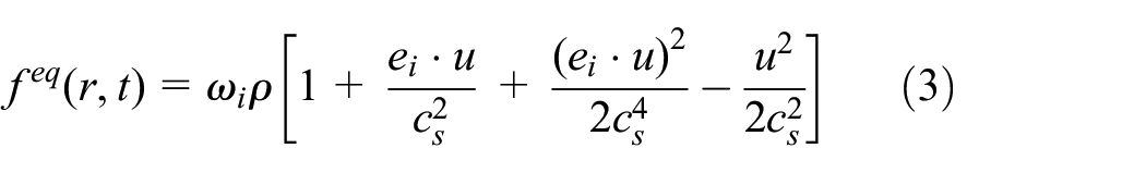
2. Distribution function definition. According to equation (3), the equilibrium distribution function can be defined. The initial distribution function is also defined with equation (3), however, it changes with each iteration.

3. Streaming and collision. The step can be achieved by use of equation (1). It should be noted that the external force item is used to explain the non-Newtonian behavior of the power-law fluid, which can be calculated with equation (18).

4. Parameter calculation. The mentioned parameter mainly refers to the viscosity, which is required for the next iteration and can be calculated by use of equations (4)–(6), (11).

5. Boundary processing. The non-equilibrium bounce-back method is adopted for processing the boundary condition, which is a common and classical method for dealing with LBM.^23,24 The wall slip is ignored here.

6. Judgment. If the velocity gap between the current with the previous step is less than 0.0001, go to (7), otherwise, go to (3).

7. Physical quantities calculation. The required physical quantities can be obtained when the simulation is finished, such as the velocity. With the program, common figures such as the velocity distributions, streamlines, can be obtained.

Figure 1.

Flow diagram.

Validation by Poiseuille flow

In the field of fluid mechanics, several cases have been solved by theoretical calculation. Poiseuille flow has the theoretical solutions for many kinds of non-Newtonian fluid, such as power-law fluid, Bingham fluid, and Herschel-Bulkley fluid. Therefore, it can be used to validate the effectiveness of the numerical method. Regarding the Poiseuille flow, the two plates are parallel to each other. For the power-law fluid, the theoretical solution of the outlet velocity is expressed as follows:

$$u_p(y)=\frac{n}{n+1}{(-\frac{1}{{\mu }_{p0}}\frac{\partial P}{\partial x})}^{1/n}[{\left(\frac{H}{2}\right)}^{(n+1)/n}-{\left|y\right|}^{(n+1)/n}]$$

(19)

where H describes the distance between two parallel plates, y is the vertical position of a certain point, ∂P/∂x denotes the inlet pressure gradient.

In the numerical simulation, the parameters are set as follows. Both the physical distance H and length L are set to 1. The lattice nodes are set to 150 × 150, the pressure gradient ∂P/∂x is set to −3 × 10⁻³, the viscosity coefficient μ_p0 is 0.01. To validate the feasibility of the method, different power-law indexes are investigated and discussed. The comparison between the numerical solutions and the theoretical solutions is shown in Figure 2. When the power-law index is set to 0.5, 1.0, and 1.5, the results show a good consistency, which demonstrates the effectiveness of the mentioned numerical method.

Figure 2.

Numerical and theoretical solutions for power-law Poiseuille flow with n = 0.5, 1.0, and 1.5.

Flow analysis in the microchannel

Microchannel manufactured by SLA

As mentioned in the Introduction, the stair effect always occurs in AM technologies. SLA, as a kind of high-accurate molding method, can be used to form the micro-parts, while the stair effect is unavoidable. It is necessary to analyze the flow in the microchannel and investigate the influence of the stairs on the flow. When the microchannel shown in Figure 3(a) is formed, the left and the right edges are printed as the first and the final layers, respectively, where the thickness is set to 0.4 mm. The geometry of the stair effect is described as the semi-circle, whose radius is 30 nm. Owing to the stair almost occurs in each layer, the semi-circles are distributed uniformly along the printing direction, which is shown in Figure 3(b).

Figure 3.

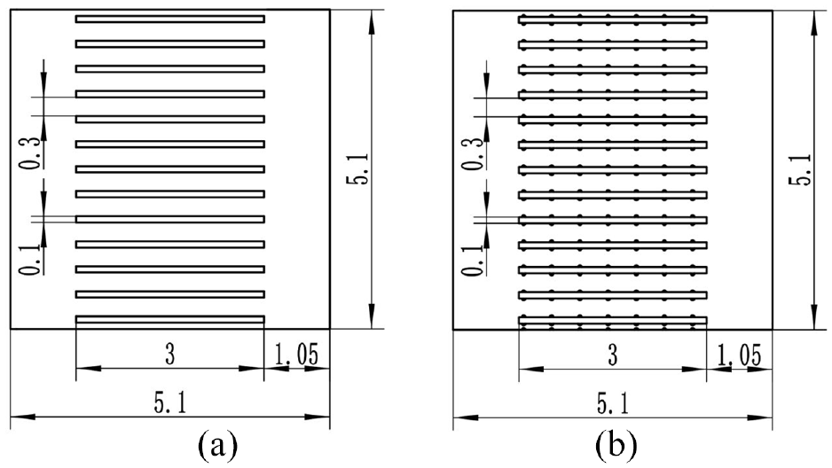
Geometry of the manufactured microchannel: (a) microchannel without stair effects and (b) microchannel with stair effects.

Flow analysis

In the simulation, the fluid flows into the microchannel from the left, and the inlet velocity is set as a parabola, whose maximum value is 1 m/s. To clearly understand the stair effects on the flow, shear-thinning, Newtonian, and shear-thickening fluids are simulated respectively. The rheological equation of the fluid is set as follows:

$${\mu }_p=0.01|\stackrel{·}{\gamma }{|}^{n-1}$$

(20)

For the shear-thinning cases, the power-law indexes are set to 0.4 and 0.8. Regarding the shear-thickening fluid, the power-law indexes are set to 1.4 and 1.8. The special case of n = 1 is also considered, which corresponds to Newtonian fluid.

Grid independency test

To validate the grid independence, the case of n = 0.4 is investigated, and the stair effect is not considered. The lattice numbers are set as 100 × 100, 200 × 200, 250 × 250, and 300 × 300, respectively. The outlet velocity of the center position for each case is given in Table 1. The results indicate that the velocity is kept almost unchanged when the lattice numbers increase to 200 × 200. Therefore, the lattice numbers should be larger than 200 × 200 to ensure that the simulation is independent of the lattice numbers. In the following simulations, the lattice numbers are set to 340 × 340.

Table 1.

The outlet velocity of the center position.

Lattice numbers	Velocity (m/s)
100 × 100	1.6956
200 × 200	1.7435
250 × 250	1.7446
300 × 300	1.7446

Shear-thinning cases

When n = 0.4, two cases are simulated for comparison. In Figure 4, the streamlines figures are given, where Figure 4(a) does not include the stairs, while Figure 4(b) considers the stair effect. The results show that the flow is smooth if there are no stairs, while the streamlines are curved in Figure 4(b) because that the flow encounters the stairs. Then, the outlet velocity distribution is given in Figure 5, which implies that when the fluid flows through the microchannel, the velocity increases. Furthermore, when the stair effect is considered, the outlet velocity increases more greatly, and the waves are more obvious.

Figure 4.

Streamlines of the case n = 0.4: (a) stair effect is not considered and (b) stair effect is considered.

Figure 5.

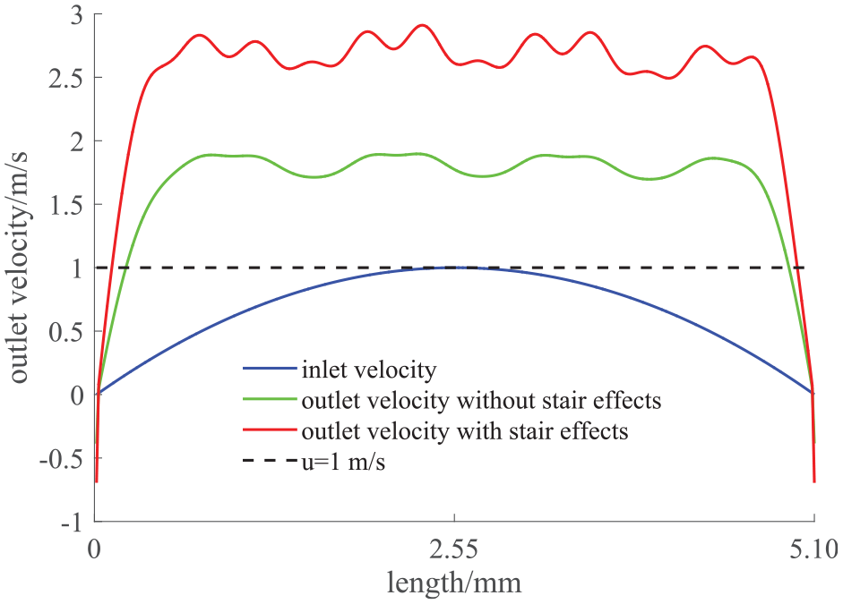
Outlet velocity of the case n = 0.4.

When n = 0.8, the comparison results are shown in Figure 6. The stairs make the streamlines curve, which is similar to the above case. In addition, the color in Figure 6(a) shows that the flow is more forceful than that in Figure 6(b). The outlet velocity shown in Figure 7 floats up and down around u = 1.0 m/s. The obvious peak and valley areas appear in the figure. The outlet velocity is slightly increased when the stair effect is considered.

Figure 6.

Streamlines of the case n = 0.8: (a) stair effect is not considered and (b) stair effect is considered.

Figure 7.

Outlet velocity of the case n = 0.8.

Newtonian case

In equation (20), when the power-law index n = 1, the dynamic viscosity is a constant, and the fluid exhibits Newtonian behavior. The results of the simulation are shown in Figures 8 and 9. In Figure 8, the streamlines are presented, which shows a similar flow phenomenon with the above cases, while the velocity distribution given in Figure 9 is different. The maximum outlet velocity is less than the maximum inlet velocity of 1 m/s in each case. According to Figures 5, 7 and 9, the outlet velocity tends to decrease as the power-law index increases. When the stair effect is considered, the outlet velocity is only slightly larger than that the stair effect is not considered. Therefore, the power-law index may be the main reason for the difference.

Figure 8.

Streamlines of the case n = 1.0: (a) stair effect is not considered and (b) stair effect is considered.

Figure 9.

Outlet velocity of the case n = 1.0.

Shear-thickening cases

When n > 1, the fluid belongs to the shear-thickening type. In Figures 10 and 11, the simulation results of the case of n = 1.4 are shown. The difference of the streamlines (Figure 10) mainly in the outlet, the positions of the streamlines have changed. The velocity distribution shown in Figure 11 presents a great difference. The peak-valley gap is more obvious than that in the above shear-thinning or Newtonian cases. There is no apparent difference in the outlet velocity curves whether the stair effect is considered or not.

Figure 10.

Streamlines of the case n = 1.4: (a) stair effect is not considered and (b) stair effect is considered.

Figure 11.

Outlet velocity of the case n = 1.4.

When n = 1.8, the simulation results are shown in Figures 12 and 13. For both the streamlines and outlet velocity, the obvious differences are presented. The streamlines in Figure 12 tend to flow to the middle position. The small vortices generate at the top and bottom position near the outlet. It implies that the negative velocity near the boundary shown in Figure 13 is decreased first and then increased, which is different from any other case in the change form although the negative velocity may also occur in other cases. The velocity curve is not smooth in the middle positions of the outlet. In addition, two curves in Figure 13 are much closer than those in other cases.

Figure 12.

Streamlines of the case n = 1.8: (a) stair effect is not considered and (b) stair effect is considered.

Figure 13.

Outlet velocity of the case n = 1.8.

Discussion

The cases with different power-law indexes are considered and explored to study the stair effect on the power-law flow in the microchannel. To conduct the numerical simulations, a modified LBM is proposed and validated. According to the obtained streamlines and outlet velocity distributions, common conclusions can be acquired when the stair effect is considered and not. The negative outlet velocity appears near the top and bottom boundaries, then the velocity increases rapidly to achieve a relatively stable value, and finally, the curve floats up and down around the mentioned value, which is quite different from the inlet velocity curve. The streamlines of the cases without stairs are smooth while those of the cases with stairs are curved.

When the effect of the power-law index on the flow is considered, some obvious differences can be found. With the increase of the power-law index, the outlet velocity decreases. In the case of n = 0.4, the outlet velocity is much larger than the inlet velocity. As mentioned above, the outlet velocity increases rapidly to reach a relatively stable value, and then the curve floats up and down around it. It is mentioned that the oscillation extent is different from each other. When n is not larger than 1, the obvious peak and valley areas appear in the outlet velocity distributions. In the peak or valley area, the curve also floats up and down, which is caused by the interactive effect of the flows between two adjacent channels. However, when the fluid belongs to the shear-thickening type, the curve of the outlet velocity is similar to the trigonometric function, which is resulted from that there is no interactive effect between two adjacent channels. Particularly, the outlet velocity of case n = 1.8 is unstable in the middle positions, and the fluid flows toward the middle position.

Furthermore, in the figures of the outlet velocity distributions, the different colors are used to distinguish whether the stair effect is considered or not. The red color represents that the stair effect is considered, and the green color represents that the stair effect is not investigated. In all cases, the red curve is located upon the green curve. The gap between the two curves in the case of n = 0.4 is much larger than that in the other cases, which implies that the stairs can increase the outlet velocity to some extent, and the small power-law index may greatly increase the velocity.

Conclusion

The stair effect always occurs in the parts manufactured by SLA. When the microchannel is printed by SLA, the stairs may affect the flow in the channels. The work mainly investigates the effect of the stairs on the power-law flow in the microchannel. A modified LBM is proposed to improve the stability for simulating non-Newtonian flow and used to analyze the mentioned cases. The results show that both the stairs and the power-law index have significant effects on the flow. The small power-law index can greatly increase the outlet velocity, while the large power-law index makes the velocity unstable.