A position control-based approach to haptic rendering of stiff objects using piece-wise linear model

Abstract

In traditional force rendering approaches, it is quite popular to model a virtual stiff wall as a spring-damper system to compute the interaction force, which can easily lead to unstable behavior. In this paper, we present an approach to ensure no penetration into the wall by position control. The approach approximates the nonlinear model of a 6-DOF parallel-structure haptic device by a piece-wise linear model to improve the performance compared with a controller designed from a one-point linearized model in haptic rendering. A simulation-based performance comparison study shows that the new controller can render higher stiffness than the previous solution.

Introduction

Haptic feedback, also referred to as the sense of touch, is one of the most important senses for human. As the electronics are getting smaller and more powerful, it can be seen in applications from the tactile motor in mobile phones to mimic a key press, to game controllers that bring more immersive gameplay through vibrations. Along that line, more specified tools like research devices,^1,2 wearable haptic gloves,^3,4 dental simulators, ⁵ and other augmented/mixed reality devices^6,7 are also developed for research and training. Although the benefits of having extra haptic feedback in some of these cases are still debatable, haptic feedback is something we rely on when we try to learn motor skills and it is hard to be fully replaced by visual and/or audio feedback.

Haptic rendering, as an analogy to graphic rendering, is the process of “displaying” an object haptically for the user to perceive through haptic channels. There is a good parallel between graphic and haptic rendering and many ideas and methods can be borrowed from one to the other. In most applications, the two also happen simultaneously for the user to have a coherent feeling of the virtual object. Properties like geometry, stiffness, and texture of the rendered object are more important in haptic rendering, while geometry, color, and shading in graphic rendering. It is commonly accepted that the haptic rendering loop should be running at 1000 Hz refresh rate to achieve realistic rendering and the loop consists of five steps: joint space position sensing, workspace position computing, collision detection, interaction force computing, and control input computing. ⁸

Haptic rendering is a challenging topic and it has many layers and aspects. Zilles and Salisbury ⁹ develop the idea of god object to better determine where the interaction is. In this case, a god object that is fully controlled and perfectly tracked is established to represent where the interaction should be and it is solved based on active constraints as the objects are using polyhedral representations. Based on this idea, Ortega et al. ¹⁰ later extend it into 6 DOFs and separate the computation for god object motion from the computation for the rendering force. They also introduce a constraint-based force computation approach, which suppresses force artifacts that exist in previous approaches. Otaduy and Lin ¹¹ propose an approach to render complex objects with high polygon count. The approach aims for both stability and transparency by maximizing the haptic refresh rate, which is achieved by linearization of the contact model in complex contact scenarios. Yu et al. ¹² propose an extended version of the configuration-based optimization approach ¹³ to render objects with fine features as well as sharp geometric features. The approach uses a coarse-to-fine sphere tree to represent an object for faster collision detection and contact constraint formulation. It is designed for dental simulators and claimed to be better for rendering narrow space constraints found in cavities and fine features like ridges on a tooth.

The aforementioned approaches mostly focus on steps in the haptic rendering loop up to collision detection with different kinds of model representations. Other researchers also explore approaches dealing with the last two steps of the rendering loop to achieve a realistic force feedback and a stable behavior when rendering stiff objects. Due to the sampling nature of the haptic device, extra energy can be generated from a passive virtual environment during interaction, which introduces instability. Gillespie and Cutkosky ¹⁴ term the phenomenon “energy leak” and they propose passivity-based approaches to solve this. Hannaford and Ryu ¹⁵ propose time-domain passivity control to achieve adaptive damping to dissipate the extra energy. Ryu and Yoon ¹⁶ extend this into a memory-based passivity approach by eliminating the energy generation from examining position versus force trajectory plot. By fast recording all the data for the plot with specially designed hardware, this method guarantees the net energy coming from the passive virtual environment is less than 0. Their controller emphasizes more on stability than transparency so the resulted behavior is a bit conservative. Colgate et al. ¹⁷ propose “virtual coupling” as a filter between the simulation model and the real device to achieve stable behavior. This approach requires the simulation to be discrete time passive, which is achieved by starting with a continuous time passive model and then discretize it using a backwards difference method if implicit equations are allowed. Adams and Hannaford ¹⁸ later extend this approach to work for both impedance and admittance models of haptic interaction but the approach is not sufficient for a dynamically changing environment. Arbabtafti et al. ¹⁹ present an approach based on the energy consumption principles behind traditional machining (removing material) to calculate the interactive force for drilling and milling in bone or dental surgery. Note that this is a 3-DOF approach because the tools for this type of operation are generally considered as a point or sphere. Desai et al. ²⁰ present a model matching framework for haptic control as they formulate the design problem as a sequence of H-infinity optimization problems. It is reported that they have stably rendered a virtual wall with stiffness up to 5000 N/m, a value well beyond stability limits suggested by other papers^17,21 based on their device.

In summary, there are different ways to capture collision and determine the interaction point. However, most interaction force computing approaches treat a virtual wall as a spring-damper system and this can lead to unstable behavior when rendering a stiff wall. In our previous work, we have proposed a position controller as a solution to achieve a stable interaction with stiff objects. ²² However, a close examination of the previous result shows that there is a tendency of performance drop when the interaction point moves from upper half to lower half of the wall, which might be caused by the increasing modeling error. In this paper, we continue to explore this idea and introduce a piece-wise linear model as the control plant in the hope of reducing that error. The following research questions (RQs) will be further explored:

• RQ 1: Can haptic rendering of stiff interaction be solved as a position controller design problem using a piece-wise linear model as a plant model?

• RQ 2: What is the effect of using a piece-wise linear model instead of one single linear model as the plant model when designing the position controller?

These RQs will be explored in the following sections.

Description of test cases

The test case for this paper is a desktop 6-DOF parallel-structure haptic device called TAU that has been previously developed at KTH for virtual dental training^23,24 and it is chosen for its complexity in structure as well as in modeling. It is a general parallel mechanism (PM) that contains a base (I-column) that is fixed to the ground, a moving platform with a tool handle, and several chains that connect the two, which then create kinematic closed loops. This is opposed to serial manipulators which only have one chain or kinematic open loop. TAU has three kinematic chains that are not identical to each other (see Figure 1) as opposed to other well-studied structure like Stewart-Gough platform, ²⁵ Agile-Wrist, ²⁶ or epicyclic systems. ²⁷ Although the chains are different, we always name the link connected to the base “link 1” with length $L_1$ and the one connected to the platform “link 2” with length $L_2$ . In chain 1 and 2, there is also a “link 3” with length $L_3$ , as indicated in Figure 1. Such asymmetric structure differentiates TAU from those well-known PMs and also results in a more complex and computationally heavy dynamic model, making it a good test case for the purpose of this paper.

Figure 1.

Kinematic diagram of TAU.

TAU has a light-weight design and each chain has two actuators close to or fixed onto the base to minimize mass and inertia effect on the moving platform.

Device specifications

The TAU haptic device is developed with the aim to provide force/torque (F/T) feedback to help dental students develop necessary motor skills for the real dental operations while training in a simulated virtual environment (VE). For this type of applications, the moving platform is equipped with a tool handle that emulates the surgical tool handle for the trainee and the tool center point (TCP) is defined at the center of the platform. The device is designed and optimized to have a workspace of a 50 mm cube that is singularity-free while keeping a small footprint for the device. The device can fit in a $250\times 250\times 300$  mm ³ box. The origin for the workspace coordinate frame is defined to be in the center of the cubic workspace. Within the workspace, the rotation range for the tool handle is $\pm 10$ ° along all axes with respect to (w.r.t) the initial pose. A schematic of the kinematic structure with the main design parameters is given in Figure 1 and the design parameter values are given in Table 1.

Table 1.

Design parameters.

Parameter	Value
Radius of the platform, $R_p$	55 mm
Length of link 1, $L_1$	138 mm
Length of link 2, $L_2$	180 mm
Length of link 3, $L_3$	91.5 mm
Length of column I, $3L_3$	274.5 mm

Definitions in kinematic and dynamic model

The task of haptic rendering can be treated as a simple control problem: given the TCP motion in the Cartesian space, driven by both the user and the device itself, design a controller that generates a motor torque reference so that the user feels the right haptic feedback. Without losing generality or consistency with previous work, ²³ the TCP pose in Cartesian space can be represented by a 6-by-1 vector

$$\mathit{X}=[p_x,p_y,p_z,\alpha ,\beta ,\gamma {]}^T$$

where $(p_x,p_y,p_z)$ denotes the position coordinates and $(\alpha ,\beta ,\gamma )$ the orientation angles of the tool along x, y, and z axis, respectively. The motion of the TCP is actuated by the active joints and the mapping from Cartesian space to joint space representation is the inverse kinematics. In the joint space, the pose of the device is also defined by a 6-by-1 vector

$$\mathit{q}=[q_1,q_2,q_3,q_4,q_5,q_6{]}^T$$

(1)

where $q_i$ denotes the angular position of joint $i$ . These are the active joints that govern the motion of the device while the rest of the joints are passive. Accordingly, the force to be rendered here is a 6-DOF force acting on TCP in Cartesian space, defined by a 6-by-1 vector

$$\mathit{F}=[F_x,F_y,F_z,T_x,T_y,T_z{]}^T$$

and the joint torque to achieve that is defined as

$$\mathit{\tau }=[{\tau }_1,{\tau }_2,{\tau }_3,{\tau }_4,{\tau }_5,{\tau }_6{]}^T$$

(2)

where ${\tau }_i$ denotes the joint torque on joint $i$ . The mapping between $\tau$ and $\mathbf{F}$ is the Jacobian matrix $\mathbf{J}$ , which is commonly found in kinematics studies and calculated in the previous work. ²³

$$\mathit{\tau }=\mathit{J}(\mathit{q}{)}^T\mathit{F}$$

Recap of position control-based approach

The idea of a position control-based approach originates in the fact that common rendering approaches usually treat a virtual stiff wall as a spring-damper system. In our previous paper, we propose a position control approach to improve the haptic rendering of a stiff wall.

In this paper, we improve the approach by using a piece-wise linear model and our scenario is still rendering an ideal stiff wall with infinite stiffness, which is an important scenario for haptic rendering. ¹⁷ If the wall is ideal with infinite stiffness, the TCP cannot penetrate or deform it. In this way, we can design a position controller to make sure that once the collision occurs, the position of the TCP is regulated at the contacting position by the position controller. As indicated in Figure 2, the input and output of the proposed controller are still the same as the traditional one but instead of estimating the interaction force in the Cartesian space, the controller guarantees no penetration (in position) to automatically generate the joint torque needed to achieve that.

Figure 2.

Illustration of the proposed method.

The goal of the controller is to prevent the TCP from penetrating into the stiff wall. Here, we consider user-applied force as disturbance instead of input to the system. Because the proposed position controller is to keep the TCP static, it will try to reject the effect of the user-applied force to the TCP by commanding the actuators to output an equal but opposite force, which is the desired force to render in this case. The TCP shall not move if the user-applied force can be counteracted without saturating the actuators. Thus, the output of the position controller is equivalent to that of a haptic rendering algorithm of a stiff wall. By turning a haptic rendering problem into a position control problem, all methods developed for position control can be applied to solve this haptic rendering problem. Note that the control goal is in the Cartesian space while the control happens in joint space since the motion of the TCP is estimated from joint encoder readings. Therefore, the position reference in the Cartesian space is mapped into joint space by the inverse kinematics of TAU.

Plant modeling

In our previous paper, ²² we present in detail the procedure to design such position controller, from plant model generation to controller design. Specifically, a model of the device is built using the Simscape module in the MATLAB/Simulink environment because of its support of modeling PMs. There are other software ²⁸ that is capable of PM modeling as well but we consider Simscape sufficient for the current requirement and well-suited for the next step in which the control plant model is linearized at one operating point (OP) with the help of Linear Analysis Tool (LAT) in MATLAB. The result of the LAT is a linear time invariant (LTI) state-space model control plant that can be expressed in general form of

$$\{\begin{array}{cc}\multicolumn{1}{c}{\stackrel{·}{\mathit{x}}}& =\mathit{Ax}+\mathit{Bu}\hfill \\ \multicolumn{1}{c}{\mathit{y}}& =\mathit{Cx}\hfill \end{array}$$

(3)

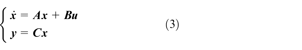
where the control input $\mathit{u}=\mathit{\tau }$ as defined in equation (2) and the output is $\mathit{y}=[{\stackrel{·}{\mathit{q}}}^T,{\mathit{q}}^T{]}^T$ , where q is defined in equation (1). The $\mathit{A}$ , $\mathit{B}$ , and $\mathit{C}$ matrices are the constant coefficients in this form. The state vector $\mathit{x}$ is a $12\times 1$ vector decided by LAT.

Because the model is obtained based on an OP, it should be w.r.t the OP with

$$\{\begin{array}{cc}\multicolumn{1}{c}{\delta \stackrel{·}{\mathit{x}}}& =\mathit{A}\delta \mathit{x}+\mathit{B}\delta \mathit{u}\hfill \\ \multicolumn{1}{c}{\delta \mathit{y}}& =\mathit{C}\delta \mathit{x}\hfill \end{array}$$

where the $\delta$ denotes the difference between the actual value and the value at the OP, for example,

$$\delta \mathit{x}=\mathit{x}-{\mathit{x}}_{\mathrm{OP}}$$

This is also done to $\mathit{u},\mathit{y}$ and later to other terms like $\mathbf{q}$ , their derivatives, and their discrete time counterparts.

The linearized model is then transformed to have the new state vector $\delta \tilde{\mathit{x}}=\delta \mathit{y}=[\delta {\stackrel{·}{\mathit{q}}}^T,\delta {\mathit{q}}^T{]}^T$ with a tilde on top as an indication. The transformed model still has the form of equation (3) where

$$\tilde{\mathit{A}}=\mathit{CA}{\mathit{C}}^{-1},\tilde{\mathit{B}}=\mathit{CB},\tilde{\mathit{C}}=\mathit{I}$$

with $\mathit{I}$ being the identity matrix and the input and output unchanged. In implementation, $\mathit{C}$ is always checked to be invertible.

Next, we augment the transformed model to eliminate the steady-state error. ²⁹ The augmented state vector, denoted by a subscript of a, is

$$\delta {\mathit{x}}_a=[\delta {\tilde{\mathit{x}}}^T,\delta {\mathit{x}}_I^T{]}^T$$

where

$$\delta {\mathit{x}}_I=\int (\delta \mathit{r}-\delta \mathit{q})\mathrm{dt}=\int (\mathit{r}-\mathit{q})\mathrm{dt}$$

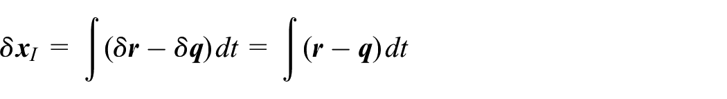
which is the integration of the error between the reference signal $\mathbf{r}$ and encoder reading $\mathbf{q}$ over time.

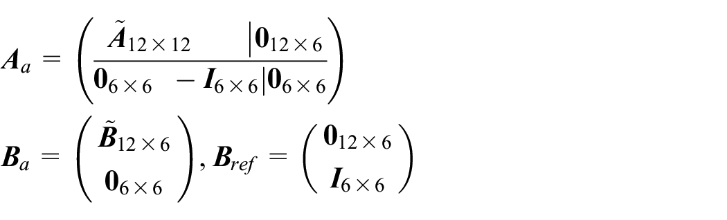
Correspondingly, the augmented model becomes

$$\delta {\stackrel{·}{\mathit{x}}}_a={\mathit{A}}_a\delta {\mathit{x}}_a+{\mathit{B}}_a\delta \mathit{u}+{\mathit{B}}_{\mathrm{ref}}\delta \mathit{r}$$

(4)

with

$$\begin{array}{c}{\mathit{A}}_a=\left(\frac{{\tilde{\mathit{A}}}_{12\times 12}|0_{12\times 6}}{0_{6\times 6}-{\mathit{I}}_{6\times 6}|0_{6\times 6}}\right)\hfill \\ {\mathit{B}}_a=\left(\begin{array}{c}{\tilde{\mathit{B}}}_{12\times 6}\hfill \\ \multicolumn{1}{c}{0_{6\times 6}}\end{array}\right),{\mathit{B}}_{\mathrm{ref}}=\left(\begin{array}{c}{0}_{12\times 6}\hfill \\ \multicolumn{1}{c}{{\mathit{I}}_{6\times 6}}\end{array}\right)\hfill \end{array}$$

Finally, a discrete time model of the augmented model is obtained by the Zero-Order Hold (ZOH) method, which implies

$$\mathit{u}(t)=\mathit{u}[j],j{T}_s\le t\le (j+1)T_s$$

where $T_s$ is the sampling time and it is set to be 1 ms (1000 Hz refresh rate).^21,30 The model from equation (4) is transformed into

$$\begin{array}{c}\multicolumn{1}{c}{\delta {\mathit{x}}_a[j+1]={\mathit{A}}_{\mathrm{aDT}}\delta {\mathit{x}}_a[j]+{\mathit{B}}_{\mathrm{aDT}}\delta \mathit{u}[j]}\\ +{\mathit{B}}_{\mathrm{refDT}}\delta \mathit{r}[j]\hfill \end{array}$$

where

$$\begin{array}{cc}\multicolumn{1}{c}{{\mathit{A}}_{\mathrm{aDT}}}& =e^{A_a{T}_s}\hfill \\ \multicolumn{1}{c}{{\mathit{B}}_{\mathrm{aDT}}}& =\left({\int }_0^{T_s}{e}^{A_{a}t}\mathrm{dt}\right){\mathit{B}}_a\hfill \\ \multicolumn{1}{c}{{\mathit{B}}_{\mathrm{refDT}}}& =\left({\int }_0^{T_s}{e}^{A_{a}t}\mathrm{dt}\right){\mathit{B}}_{\mathrm{ref}}\hfill \end{array}$$

The $e$ here is the natural constant. The result is a discrete time LTI state-space model control plant, denoted by a subscript of a DT.

Control design

As discussed before, the control goal of the controller is to keep the TCP fixed at the collision point so that the deviation from that point is minimized under random disturbance. So we formulate the control problem as an optimization problem to find the optimal gain ${\mathit{K}}_{\mathrm{aDT}}$ such that the state-feedback control law

$$\delta \mathit{u}[j]=-{\mathit{K}}_{\mathrm{aDT}}\delta {\mathbf{x}}_a[j]$$

minimizes, with a linear-quadratic-regulator-based (LQR-based) formulation, the quadratic cost function

$$\mathrm{cost}(\delta \mathit{u})=\sum _{j=1}^{\infty }(\delta {\mathit{x}}_a^T[j]\mathit{Q}\delta {\mathit{x}}_a[j]+\delta {\mathit{u}}^T[j]\mathit{R}\delta \mathit{u}[j])$$

The $\mathit{Q}$ and $\mathit{R}$ matrices are initialized as identity matrices and tuned to be

$$\begin{array}{c}\mathit{Q}=\left(\begin{array}{ccc}{\mathit{I}}_{6\times 6}\hfill & 0_{6\times 6}\hfill & 0_{6\times 6}\hfill \\ \multicolumn{1}{c}{0_{6\times 6}}& {10}^3\times {\mathit{I}}_{6\times 6}\hfill & 0_{6\times 6}\hfill \\ \multicolumn{1}{c}{0_{6\times 6}}& 0_{6\times 6}\hfill & {10}^7\times {\mathit{I}}_{6\times 6}\hfill \end{array}\right)\hfill \\ \multicolumn{1}{c}{\mathit{R}={\mathit{I}}_{6\times 6}}\end{array}$$

Piece-wise linear model extension

In this paper, we explore the effect of modeling the control plant as a piece-wise linear model. Motivated by the performance drop in the region far away from the only one OP during previous simulations, more OPs are established on the edge of the workspace. Because the workspace of the device is a $50\times 50\times 50$  mm ³ cube, the center point of the cube, all the vertices, and all the middle points on the edges, a total of 27 points, are chosen to be the OPs for the purpose of this paper. The OPs (see Figure 3) are shown as follows

$$\begin{array}{c}{{}^{\mathrm{OP}}\mathit{X}}^{m,n,l}=\left(\begin{array}{c}{{}^{\mathrm{OP}}p}_x^{m,n,l}\hfill \\ \multicolumn{1}{c}{{{}^{\mathrm{OP}}p}_y^{m,n,l}}\\ \multicolumn{1}{c}{{{}^{\mathrm{OP}}p}_z^{m,n,l}}\\ \multicolumn{1}{c}{0_{3\times 1}}\end{array}\right)=\left(\begin{array}{c}25(m-2)\hfill \\ \multicolumn{1}{c}{25(n-2)}\\ \multicolumn{1}{c}{25(l-2)}\\ \multicolumn{1}{c}{0_{3\times 1}}\end{array}\right),\hfill \\ \multicolumn{1}{c}{m,n,l\in \{1,2,3\}}\end{array}$$

Figure 3.

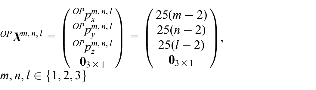
Illustration of the workspace (blue box), the wall (green surface), 27 OPs (red dots), and a grid of QPs on the wall.

where $m,n,l$ is the OP index in $x,y,z$ direction, respectively.

Accordingly, 27 plant models are generated based on these OPs using the same procedure mentioned above and 27 controllers are designed with the same $\mathit{Q}$ , $\mathit{R}$ matrices. So the new controller is actually a collection of 27 sets controller gains. In this way, when the device is operating at a point far away from the center of the workspace, it can use the controller that is generated based on a closer OP. In the simulations shown later, we will query the performance of the whole system at a grid of points, which are called query points (QPs). These QPs should be the result of collision detection as it is the point of interaction. Thus, the problem of which controller to use is formulated into finding the closest OP based on the current QP. There are different ways to define the distance between two points and to search for the shortest among multiple pairs. In this paper, we start by growing cube-shaped subspaces around the OPs so that each OP is at the center of its subspace and the sizes of all subspaces are the same. Then, we determine which subspace the QP is in by checking its x, y, and z coordinate, respectively. The checking rule for each coordinate can be written as

$${{}^{\mathrm{OP}}p}_i=\{\begin{array}{c}-25,-37.5<{{}^{\mathrm{QP}}p}_i<-12.5\hfill \\ \multicolumn{1}{c}{0,-12.5\le {{}^{\mathrm{QP}}p}_i\le 12.5,i\in \{x,y,z\}}\\ \multicolumn{1}{c}{25,12.5<{{}^{\mathrm{QP}}p}_i<37.5}\end{array}$$

It should be noted that the total volume of all subspaces exceeds the workspace of TAU but the position of the QP is also subjected to the boundaries of the workspace. We choose this method to have less computation, which is important for real-time applications. Note that the transition among these controllers is not considered in this paper as the tool is not moving along the wall. It can be an interesting topic for later. For comparison, we choose the better performance controller in the previous paper, ²² which is referred as the proposed controller in that paper, as a baseline. However, we call it the single-operating-point controller (SOPC) in this paper to highlight that it is generated from a control plant using a single OP. Our newly proposed one is named multiple-operating-point controller (MOPC), respectively.

Simulation methodology

To investigate the effect of using a piece-wise linear model as the control plant, we perform the same simulation for both SOPC and MOPC with the help of MATLAB/Simulink. By using this environment, we can reuse the full dynamic model of the device, which is developed to generate linearized model. Furthermore, all aspects of the simulation can be specified by MATLAB scripts, which is good for running a large number of Monte-Carlo simulations with slightly different setting parameters. The virtual wall is considered a unilateral constraint, similar to the definitions by Desai et al. ²⁰ As stated previously, the simulation uses the full (dynamics) model of the device and the linearized model is only used in designing the controller. In other words, we design controllers based on linearized models and test the performance of the controllers on the full model. Because we formulate the haptic rendering problem into a position control problem, the user force exerted on the TCP is considered a disturbance to the controller. The purpose of the simulation is to investigate how well the controller can keep the TCP position under various disturbance forces and what stiffness it can render. To capture the response to sudden disturbance, we have chosen a step force signal as the disturbance. Because we are rendering a flat wall parallel with xy-plane, the disturbance is always along z axis toward the wall, imitating a push on the tool to press against the wall.

The wall we are rendering is located at $z=0$ , on which we have defined a grid of uniformly distributed QPs. The x and y coordinate of the QPs range from −25 to 25 mm with a step of 5 mm, resulting in a grid of 121 QPs on the wall (Figure 3). We query the performance of the controller at each QP by running the same simulation repetitively to have a performance distribution over the rendered wall. The simulation is conducted as follows: the TCP is first initialized at a QP, in contact with the virtual wall but with no interaction force, which is the boundary case for collision detection. Then, a disturbance signal is applied and the response of the system will be recorded and later analyzed. This is the simulation setup for both controllers. It should be noted that for MOPC, once the system is initialized, a controller based on the OP closest to the current QP is chosen.

For the simulation, the disturbance signal is shown below

$$F_{\mathrm{disturb}}(t)=F_{\mathrm{signal}}(t)+w_{\mathrm{noise}}(t)$$

where

$$\begin{array}{c}{F}_{\mathrm{signal}}(t)=\{\begin{array}{c}0,0\le t<1\hfill \\ \multicolumn{1}{c}{F_c,1\le t\le 3}\end{array}\hfill \\ w_{\mathrm{noise}}(t)=\{\begin{array}{c}0,0\le t<1\hfill \\ \multicolumn{1}{c}{\mathcal{N}(0,0.5),1\le t\le 3}\end{array}\hfill \end{array}$$

The force disturbance signal consists of a step signal and a white noise. For the step signal, there is a 1 s delay for the system to stabilize itself before the step happens at time point t = 1. The step level ( $F_c$ ) is randomly generated uniformly within the range of 8–15 N for each run. The step signal holds for 2 s, until the end of the simulation. The total simulation time for a single run is 3 s. The disturbance is overlaid with a high frequency white noise signal. We use the notation $\mathcal{N}(\mu ,\sigma )$ to indicate that the noise follows normal distribution with a mean of $\mu$ and a standard deviation of $\sigma$ . The amplitude of the white noise is roughly 10% of the step level. As stated, the same simulation will be run at each QP with a randomization in the step level and added white noise as a Monte-Carlo simulation in order to check the robustness of the performance.

After finishing and recording all the simulation, we post-process each simulation run to identify maximum penetration into the wall, the stiffness value corresponded to that, and the absolute deviation in $p_z$ w.r.t its QP. Note that this is for a single simulation. And then we compile all 20 simulations at each QP to get the performance distribution over the rendered wall. As our study is purely numerical and quantitative, this simulation framework can serve as an initial step before any physical experiments to get an estimate of the performance. This estimate can be a good indication of whether or not to move to the next experimental phase which requires more careful designs to work with a variety of human users.

Simulation results

With the disturbance signal, the results demonstrate more about the response under sudden quick disturbance changes, similar to the purpose of doing a step test.

The results in Figure 4 show a similar trend and range of value for both controllers with slight differences. The stiffness value is invariant of the change in x coordinate only. With the decrease of y coordinate on the wall, the mean of stiffness also decreases. Although the range of value is similar, the result for MOPC has a higher minimal mean stiffness than that for SOPC, for about 100 N/m. The stiffness mesh for MOPC also varies less than that for SOPC.

Figure 4.

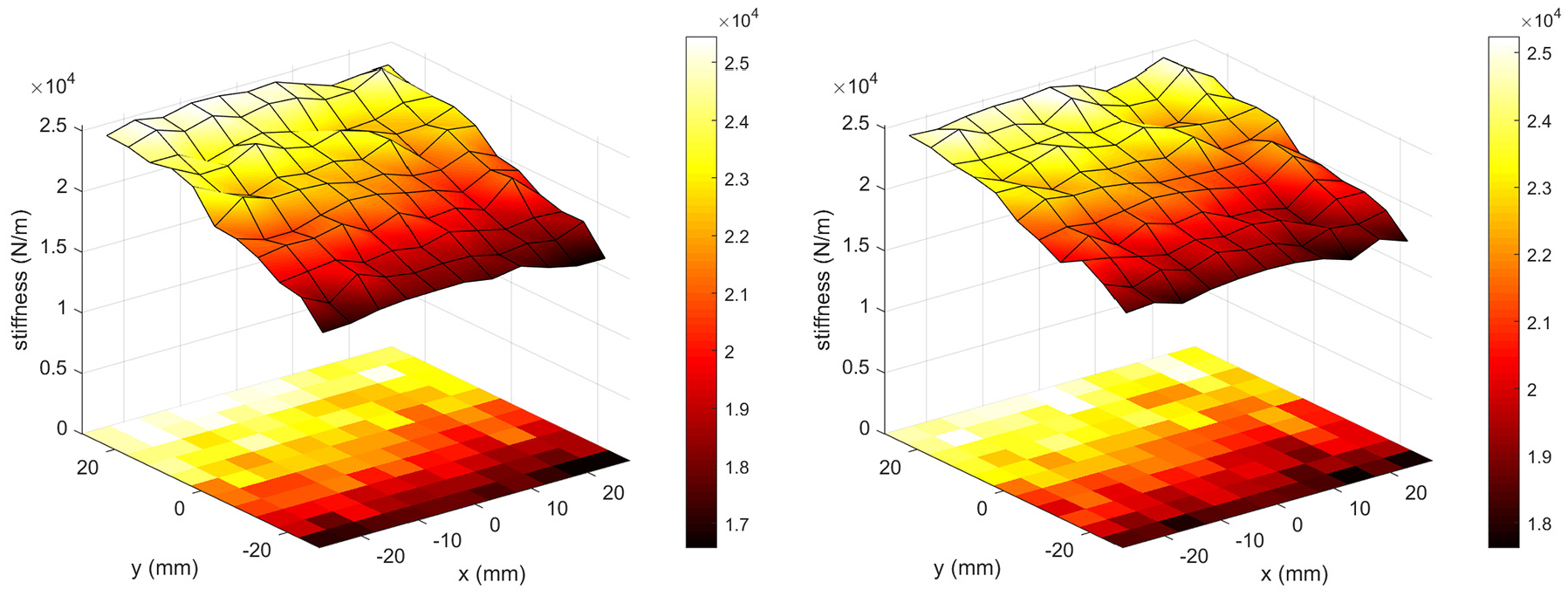
The mean stiffness over 20 simulations at each QP distributed over the wall (top: SOPC, bottom: MOPC).

Apart from the stiffness distribution over the rendered wall, we also examine simulations across all QPs and the results are summarized in Table 2. Note that the mean function is like a filter that “softens” the effect of improvement.

Table 2.

Stiffness characteristics across all simulations.

Parameter	SOPC	MOPC
Minimal stiffness (N/m)	$1.58\times {10}^4$	$1.66\times {10}^4$
Mean stiffness (N/m)	$2.15\times {10}^4$	$2.17\times {10}^4$
Standard deviation (N/m)	$2.50\times {10}^3$	$2.10\times {10}^3$

Because the results are so close to each other, we run t-tests with significance level of 0.05 on the data to see if the results are significantly different. That means we can determine whether or not we have 95 % confidence to say that the mean of the two data sets are significantly different. ³¹ Figure 5 shows which QPs show significantly different results, have higher results for MOPC, and meet both conditions. It seems that when $y<12.5$ , which is the area lower than the yellow square, the performance for MOPC is indeed improved. This improvement is found 30 out of 33 QPs, which also supports the conclusions drawn from Figure 4. Out of all 121 QPs, only 17 show higher stiffness with SOPC that is considered significant. Note that this number might be slightly affected by how the QPs are set up.

Figure 5.

Statistical result at each QP on whether the performance of the two controllers are significantly different (left), whether MOPC has a higher mean than SOPC (middle), and the intersection of the two (right). Lighter color means “true” and darker “false.”

To illustrate more details in the responses, we closely examine the nine simulations where QPs are the same as the OPs of MOPC. The position of subplots in Figure 6 corresponds to the position of the QPs on the wall. The performance at these QPs should be the best for MOPC because the model to design the controller should be accurate at that point. And for SOPC, these QPs are the furthest away from its sole OP for they are on the boundary of the workspace. As shown in the Figure 6, the deviation plots of the TCP in z axis for both controllers are again quite similar. These plots are generated with a constant disturbance signal of 13 N without noise. The plots at different QPs show a similar result. In response to the sudden disturbance, MOPC performs a bit better than SOPC, showing a smaller penetration with an average of 7.9% of improvement. The average root-mean-square errors (RMSEs) in z coordinate across nine QPs for MOPC and SOPC are 0.13 and 0.16 mm, respectively. A larger difference is actually shown when the system is initializing, where SOPC often has a short period to stabilize and MOPC holds the initial pose quite well. The plot in the center shows identical responses for both controllers, which is why the blue plot for SOPC is totally covered by the red plot for MOPC on top and is not visible.

Figure 6.

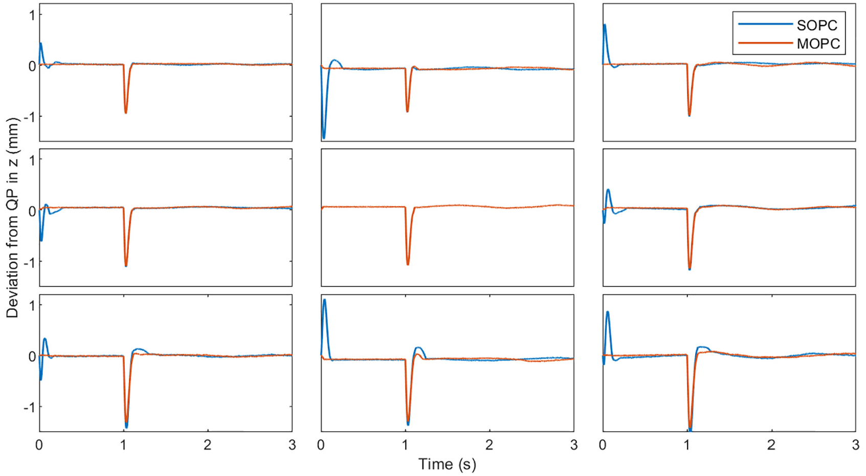
Selected nine simulations where the QPs are the same as the OPs for MOPC (with x coordinate of QPs increases to the right, y coordinate increases to the top, and the origin in the center).

Discussion

To investigate the proposed approach for haptic rendering, we have chosen to render the interaction with a stiff wall as an initial test case. This wall is at $z=0$ and parallel to the xy-plane, which enables us to study the performance solely in z axis direction.

From the stiffness distribution plot (Figure 4), we find that MOPC performs slightly better than SOPC. This advantage is more visible in the low stiffness area (small y coordinate, bottom of the wall), which gives MOPC a higher value in minimal stiffness, improving the overall performance. This is important since we have assumed earlier that the low stiffness area is due to saturation in motors and cannot be improved by a change of controller. However, it is possible that with a more detailed plant model, in our case a piece-wise linear model, the reference signal computed by our controller is further away from the saturation and easier to reach.

This is further verified by Figure 5 as the stiffness at most (30/33) of the QPs with $y<12.5$ is improved when using MOPC. The other three are the insignificant ones, meaning their result is similar to that of SOPC. Because of how MOPC is designed, when a QP is at the center region of the wall where $\{(x,y)|-12.5<x<12.5,-12.5<y<12.5\}$ , the two controllers are essentially the same as they both use the linearized model from the origin. This is also illustrated in the left image of Figure 5 since the results in that region, bounded by a yellow square, are considered not significantly different. The rest of the region on the wall, where MOPC is indeed different from SOPC, not all QPs show significant improvement. This indicates that MOPC can be further optimized to have less sets of controller gains to save some memory storage.

This advantage is achieved by saving a few more controller matrices in the memory of the controller processor. In the current case, the number of controllers dividing the workspace is still manageable. With a larger workspace and a finer division, the number and the memory space for saving can grow rapidly. However, as the result indicates, the “optimal” number of OPs for controlling TAU is probably at the level of 27 as it only improves a little compared to that of 1. A relatively small workspace can be the main reason behind this. Another possibility might be that the current rendering case of a virtual stiff wall is quite simple and the improvement of having more OPs is not that significant.

The difference illustrated in Figure 6 also aligns with the results shown in Figure 4. The performance over the rendered wall are similar for both controllers because the response to the disturbance is only marginally different, with MOPC a bit better, even at the edge of the workspace where the difference should be the largest. In addition, Figure 6 shows another advantage for MOPC that is not visible in plots like stiffness distribution over the rendered wall. The stiffness distribution plot emphasize more on disturbance rejection while this advantage exists in system initialization. The small motion with SOPC in the beginning of the simulation is basically a result of mismatch between the model used to design SOPC and the real model of the device at the current QP. This mismatch manifests into a “jerk” of the TCP and might be perceived by the user as an artifact in rendering. Fortunately, this mismatch is quickly mitigated by the integral part of the controller, leaving a steady pose as what MOPC has before the disturbance happens. In practice, the TAU device should always initialize at the origin when turned on but this effect of mismatches will still show when making initial contact far away from the OP for SOPC.

Conclusions and future work

From the discussion, we can conclude that using a piece-wise linear model as the control plant model improves the performance especially when the device is operating near the edge of the workspace, as opposed to using only one linearized model at the center of the workspace. On the other hand, the burden of this approach is that instead of having one set of controller gains, several sets are needed, of which the number grows with the number of OPs. Although this seems to suffer from the curse of dimension and the number of OPs grows fast in order to have finer division of the workspace, it is actually quite manageable in our case when one linearized model can fit the whole workspace quite well. Although the current improvement in stiffness seems to be only in the numbers and too little for a human user to notice, MOPC shows a significant improvement in the lower area of the wall, where improvement is needed the most. We argue that this improvement may be more significant when the rendering case is more complex or demanding. For this paper in particular, the rendered wall is at the center of the workspace and perpendicular to z axis, leaving the device in a symmetric setup. A more demanding case for the motors can be interacting with an angled wall, which is a part of our future work. An extension to have a smooth transition among the controllers will also be explored.