State of the art methods to post-process mechanical test data to characterize the hot deformation behavior of metals

Abstract

Materials engineering and science rely heavily on the indirect measurement of plastic stress and strain by post-processing of mechanical test data, including tension, torsion, and compression test. There is no consensus among researchers regarding the best test or the post-processing theory nor do adequate standards exist on the characterization methods. The tests are typically performed as customized tests, discrepancies exist in the flow curves obtained by different methods and the chosen mechanical test. More critically, the curves are dominantly treated (perceived) as a set of measured data rather than calculated values. The plasticity-based calculated flow curves and their gradients are, in turn, the basis for several second-tier indirect measurements, such as stacking fault energy and recrystallization. Such measurements are quite prone to errors due to oversimplified post-processing of the tests’ data and can only be experimentally verified in a qualitative or in an average fashion. Therefore, their findings are highly restricted by the limitations of each test, data type and post-processing method, and should be used carefully. This review examines some of the most commonly used data conversion methods and some recent developments in the field followed by recommendations. It will highlight the need to develop test rigs that can provide new data types and to provide advanced post-processing techniques for the indirect measurement.

Introduction

Industrial metal forming processes are way too expensive to be designed and optimized via trial and error. In the last 70 years, thermo-mechanical processing in the metal forming industry has developed from a skills-based approach, relying on trial-and-error developments, to a scientific one, thanks to mathematical modeling and computational analysis to control and optimize its processes and to transfer the results from bench-scale physical simulations to real industrial production. With a rapid increase in the basic understanding of the microstructural changes’ physics and the speed of computing, more complex models have grown to enable the capacity for offline optimization, online control, and property prediction. Such models are now accepted as an economically valuable tool for thermo-mechanical processing. ¹

Parameter gaps: Industrial parameters versus physical simulation parameters

Table 1, ² demonstrates the industrial parameters for some commonly used hot rolling mill operations. It outlines the normal range of strain, strain rates, and temperatures for different types of rolling mills. Also, it presents the range of inter-deformation times. Conducting continuous rolling mill (e.g. rod, bar, and the finishing train of a hot strip mill), the strain rate and inter-deformation time are coupled; each sequential pass has a higher strain rate and a shorter inter-pass time. However, during reverse millings, such as plate mills, the inter-pass time changes along the length of the plate because the head at one pass becomes the tail end at the next. Increasing the plate length and maintaining the roll speed, the inter-pass times may increase during rolling.

Table 1.

Typical range of processing conditions for conventional hot rolling mills. ²

Mill type	Strain per pass	Total strain	Strain rate (s_1)	Temperatures (8°C)	Interpass time (s)
Plate Strip	0.05–0.4	1–4.5	0.3–30	1300–700	5–20
Finishing Roughing	0.2–0.5 0.1–1.3	~2.5 1.5–3.2	0.5–10 10–100	1300–900 1050–700	~10 1–5
Total Structural	0.05–0.8	4–5.7 1–4.5	0.3–30	1250–800	~10
Bar	0.3–0.6	2–5	0.5–300	1200–900	0.07–3
Rod	0.3–0.6	4–7	Up to 2000	1200–900	0.01–3

On the simulation front, sample temperature can be controlled with reasonable accuracy to match those of the industrial one; however, the highest strain rate that can be simulated during the mechanical tests is typically below 100 s⁻¹, which presents a large gap to be extrapolated. Typically, the Zener-Hollman parameter is used in the simulations and extrapolations that account for both temperature and strain rate at the same time. Also, the minimum achievable inter-pass time, by servo-hydraulic actuators, via the test rig is larger than 10 ms. ³ More details on the achievable ranges of the deformation parameters by physical simulations will be presented later in this review. These allow a better understanding of the gap between some of the industrial hot/warm deformation parameters for steels and those of the physical simulations reviewed here.

The pioneering work on recrystallization, by Sellars and McTegart ⁴ and Doherty et al., ⁵ has inspired numerous researchers over the past five decades, to indirectly measure sophisticated deformation phenomena, such as stacking fault energy, static recrystallization (SRX), dynamic recrystallization (DRX), and recovery, based on the mechanical behavior of the materials during the deformation. Examples of these are the effective stress, its derivative with respect to the effective strain, strain rate, and temperature. From a materials science perspective, these phenomena are typically associable with some tangible features, for example, grain size, a solution-phase such as austenite and the dislocation density. From the mechanical engineering perspective, the effective values are associated with measurable values, such as deformation load, displacement, and velocity of the deforming tool. The latter are available as “raw data” during mechanical tests, such as tension, torsion, or compression test. The indirect measurement entails a conversion of the “raw measured” data to “computed” effective stress, strain, and strain rate. The computational step employs mathematics and plasticity-based post-processing methods to account for the mechanical science aspects of the industrial processes and tests. Unfortunately, numerical methods are not currently the most convenient or feasible tools to post-process the raw data. The most commonly used tools are closed-form un-coupled solutions of the mechanical tests, which only allow a limited inclusion of the real deformation issues and phenomena in them.

While it is fully justified to utilize simplified approaches to prove a concept such as indirect measurement of softening mechanism at its early stages and simplified post-processing of the mechanical tests to measure stress, given the significant improvements in computational speed and computing frameworks, it is surprising that still simplistic approaches are widely being used in a large body of the relevant studies.

There is plenty of scope for improvements such as tools and experiments. The gaps and some of the recent developments in the field are reviewed in this article.

General notes and historical background

Material’s flow data often represented mathematically as the constitutive equation, is regarded as the key reference to physically simulate a deformation process. ⁶ It is typically presented with four important variables, namely effective stress, strain, strain rate, and temperature. The effective stress is regarded as the dependent variable and the three other variables are also known as primary parameters. Secondary parameters, which are related to microstructure and microscopic features of the crystal, are occasionally integrated with the equation as separate theoretical and mathematical layers; see, for example, Estrin and Mecking ⁷ or Brown et al. ⁸ for hot working.

The flow condition is typically represented by the maximum distortion criterion (von Mises ⁹ criterion); once the second invariant of deviatoric stress J₂ of a ductile material reaches its critical value, the material begins to yield. The criterion has also been formulated in terms of the von Mises stress, also known as the effective stress, which is equivalent to the uniaxial tensile stress in an ideal tensile test. The definition and the criterion have been used widely to predict the yielding of ductile materials subjected to multi-axial loading. The criterion, as proposed initially, does not explicitly account for the work hardening, rate hardening, or temperature dependence. To address the limitations and dependencies for a specific ductile material, several empirical equations, also known as constitutive equations, have been proposed by different researchers. Such a constitutive equation represents the effective stress mathematically as a function of its primary variables including effective strain, strain rate, and temperature. Also, other secondary equations (sub-equations) have been integrated into the constitutive equation, empirically and theoretically, to correlate each primary parameter to some secondary material-related parameters, such as the internal parameters, dislocation density, activation energy, grain size, etc. The coefficients in a constitutive equation and its secondary equations are typically calibrated using the results from a mechanical test which is assumed to be iso-thermal and based on a homogeneous deformation. More details on the history of metal forming and plasticity can be found in Osakada. ¹⁰

The first concern to utilize a constitutive equation is that none of the primary or secondary parameters in a constitutive equation is directly measurable; typically, sophisticated plasticity-based post-processing steps are needed to convert the measurable data from a physical simulation, load-displacement, into the primary or secondary parameters before their coefficients can be calibrated.

The second concern is that the above-mentioned calibrations rely highly on the average calculated effective stress, strain, and strain rate and do not account for the heterogeneity of the primary parameters during the deformation in the test sample; none of the deformation scenarios, in industrial or physical simulation level, are iso-thermal nor homogeneous.

Constitutive descriptions for high strain rate deformation processes, for example, cold or hot metal spray or rod rolling, are usually derived from oversimplified post-processing of the data acquired by orthodox mechanical tests. The constitutive parameters for more sophisticated processing of the test data are identified using optimization-based, experiment, and numerical techniques: notably the inverse solution. The inclusion of more experimental data into the experimental-numerical cost function in an inverse manner results in a more robust constitutive model.

Surprisingly, in a large amount of the current literature, the post-processing methods are usually seen as a procedural step not worthy of being discussed. Such reports may fail to deal with and address the appropriate identification of the flow curve. In these works, the calculated effective stress, strain, and strain rate values are regarded as reliably measured values rather than calculated ones. The values have been subsequently used as the reference to verify/calibrate their postulated mathematical expressions to quantify the variations and correlation of the deformation parameters together and are now being extensively used to bridge the lab-scale studies with the material behavior in industrial processes. These post-processed data have subsequently been used to explain and quantify sophisticated phenomena such as SRX, DRX, and recovery. The addition of multi-layers empirical sub-equations in these works to correlate the internal parameters of deformation can only add to the confusion while the post-processing issue is not accounted for properly.

The key point of including the early references in this work is to highlight the gap between the three following eras:

• With the beginning of mechanical tests, flow curve identification techniques were rapidly and extensively developed by some pioneers. With the advent of numerical solutions, the developments stopped abruptly and prematurely. However, the numerical methods failed to provide adequate and proper methods to identify flow curves; the flow curves are needed as an input to conduct a numerical study (these are extensively reviewed in this paper).

• Despite the immaturity and inadequacy of the existing flow curve identification methods/tests, many research groups have employed the highly questionable flow curves to justify their hypotheses on the deformation phenomenology, deformation mechanisms, texture evolution, etc. Disagreements between the identified flow curves of the same materials based on different tests and techniques have been known for many years.

• Recent developments of flow identification techniques based on both analytical and numerical-inverse methods.

Few works exist in the literature with an emphasis on the importance of post-processing. Examples for advanced post-processing include those of multi-stage rolling to measure material’s fractional softening and subsequently to calibrate its static recrystallization kinetics model works based on torsion^11–13 or compression tests data.^14–16 These studies have taken into account the non-homogeneous microstructure in their data conversions. Moreover, an optimization method composed of a numerical method and a set of experimental raw data has been used (e.g. Chen et al. ¹⁷ ) to calibrate the parameters of a pre-selected flow model.

Scope

A physical simulation via a bench-scale mechanical test (e.g. tension, torsion, compression, or split-Hopkinson pressure bar test) allows variation of load and displacement, and is meant to keep the two remaining parameters (strain rate and temperature) fixed; however, there are several practical and inherent limitations for each test to fully control strain rate and temperature. More limitations exist for the hot tension test and split-Hopkinson pressure bar, and therefore, the two tests are less used than the two others for physical simulation of the industrial processes. Also, the heterogeneous grain structure of the deformed sample makes the post-processing of the test data extremely challenging, particularly when the test simulates a multi-stage deformation path and/or when the dynamic response of the material is being simulated. Given the unique limitations and capabilities of each test and method, one can better understand the reason behind the use of several tests and methods in the current literature.

For example, there is confusion in the characterization of hot deformation via compression test (e.g. dynamic recovery (DRV), SRX, DRX, and meta-dynamic recrystallization (MDRX)), due to the use of simplistic flow curves. Reported flow curves are assumed to be closely linked to the ram velocity. The post-processing of the measured load-displacement data from the test relies on very basic and inadequate solutions and models.

While the pros and cons of each test have been known for many years, the post-processing methods have slowly evolved to convert the measured load displacement to the calculated stress-strain curve. Nevertheless, the raw data collected by each test are quite limited and, in some cases, inadequate to address the needs of new analytical methods; therefore, the methods and experiments are far from perfect.

The inclusion of the second or third-tier test conditions could have intensified this review even more. This is better visualized after noting that such “deformation mechanisms (e.g. microstructure evolution)” are specific to the material types (e.g. metallic/non-metallic) and the alloying elements and even deformation parameters such as strain, strain rate, and temperature.

Flow characterization; a pre-requisite for meaningful microstructural modeling/studies: Irrespective of the chosen test, one has to realize the fundamental role of material flow curve for any meaningful study of deformation. There is a large body of microstructural and phenomenological models to explore the real-time phenomena development during the deformation (e.g. a multi-layer, microstructure-based and real-time models ¹⁸ ). These rely on several detailed modules and a combination of direct and indirect solutions such as Cellular Automata and Finite Element method. They utilize dedicated models for micro shear and shear bands analysis and recrystallization and involve the description of various material properties in “different time and length scales.” However, such studies critically depend on the flow curves as their input. Without a valid flow characterization, such auxiliary tools/platforms are useless and invalid. Therefore, the current review is focused on the provision of valid flow curves as the input to enable a valid micro-structural study.

This review is mainly focused on the existing routine and advanced methods, while it also makes some recommendations for the test rigs of the future. Special emphasis has been laid upon the required analytical and experimental improvements in the field of axisymmetric compression testing based on the recently developed analytical solutions of the test that require new measurement types.

The review outlines

First, in this review, the common tests for flow stress measurement are outlined and the advantages and limitations of each test are highlighted, the extent of heterogeneity in their deformed samples is explored and parameters responsible for these are discussed. It will be discussed how the non-uniform deformation impacts the material’s identified flow curves for a single and multi-pass hot deformation scenario.

“Common issues in mechanical testing” and “currently used post-processing methods” are reviewed separately in sections 3 and 4, respectively as self-contained sections to allow an easier browsing of each by the reader.

The importance of this review can not be understood without exploring the industrial applications for the flow identification. We have chosen thermo-mechanical processing as of the key application for the reviewed topic. A quick glance of the work in the field of thermo-mechanical processing demonstrates the gravity of the chosen application. However, given the large extend of this application, the topic will be presented very concisely here.

The aim is to improve the accuracy of the indirect measurement by appropriately designing the tests and using advanced methods, proper experimental setups, and new data types. This enables a better indirect measurement of stress in the deformed sample under the analytically and experimentally valid conditions and eventually increases the consistency of the characterized results over different platforms and research groups.

Common mechanical tests for hot characterization

Two major issues for all metal forming processes and structural designs are the forces required for the operation and the properties of the material. Understanding the interaction between a material’s deforming loads and its properties is crucial to design a forming process or to verify the integrity of a structure under its service conditions. The required force, however, depends highly on the workpiece geometry, loading boundary conditions, tool shape, tool speed, and several other parameters; therefore, these types of measurements are not directly transferable to other processes. Before such a transformation can be performed, one has to express the measurements in terms of some universal variables such as effective stress, strain, and strain rate.

The analysis of forces (and stresses) in metal forming processes has been an active area of applied plasticity for the past 50 years. Due to the complexity of force analysis in many metal forming processes, closed-form solutions only exist for the simplest forming processes including mechanical tests. If higher accuracy is required, these analyses can be numerically performed.

Numerical simulations versus closed-form solutions

In the last decades, numerical solutions for many metal forming analyses have been developed; however, these numerical solutions are not sufficient for accurate determination of forces during deformation. Accurate and reliable constitutive equations are also required to precisely identify the forces. Knowledge of the constitutive parameters, which are used to describe relationships between forming variables such as stress, strain rate, temperature, etc., is a prerequisite to numerically determine the forces during the deformation of a material. The constitutive parameters, however, are in turn found based on simplified closed-form solutions of mechanical tests, and therefore they may not be accurate enough to calculate the forces numerically. In other words, the use of the identified set in a numerical solution can lead to inaccurate determination of the required forces for the given deformation process. Hence, one has to solve a metal forming process numerically and break this vicious circle to ensure a complete solution.

Attempts to predict and explain the behavior of materials may be categorized in several ways. They enable to complete the following steps:

1. Identifying the parameters of a given mathematical model,

2. Discovery of new phenomena or a better understanding of known phenomena during deformation of the material, and

3. Developing mathematical models to represent these phenomena.

The determination of the flow curve and its constitutive parameters falls into the third group. Accurate determination of the constitutive parameters needs a large experimental body of data and rigorous analytical tools, such as closed-form solutions and/or numerical methods. A common approach is to devise an inverse solution to use both numerical solution and experimental measurements to explain and predict the behavior of the material; see, for example, Gavrus et al. ¹⁹ , Khoddam et al. ²⁰ The inverse solution enables us to post-process the raw measured data. The experimental data required for this task are usually obtained by performing a suitable mechanical test. Further developments are needed in inverse methods to efficiently use the experimental data and to utilize robust numerical methods to analyze the experimental data. This will be discussed more in section 6 of this review.

Criteria for a good mechanical test

Years of experimentation have shown that suitable mechanical tests to determine the stress-strain relationship should satisfy the following criteria:

1. Stability of deformation. The specimens are not to fail before reaching the amount of deformation required,

2. A simple geometrical configuration over the entire test for ease of analysis, and

3. An ability to simulate hot strength parameters.

The most important mechanical tests are the tension test, hot torsion test, axisymmetric or plane strain compression tests, and the hot/cold split-Hopkinson pressure bar test. In the rest of this section, these tests are generally introduced, and their weaknesses and strengths in fulfilling the above-mentioned criteria will be discussed and compared in section 3.

Tension test

The simplest test for predicting behavior in metalworking is the tension test; however, the disadvantages of this test are the limited magnitude of attainable homogeneous deformation compared with that of the other tests. The limitations are posed by the occurrence of necking during the early stages of deformation in the test sample. The post-necking conditions do not fulfill the second requirement outlined in section 2.2. The status of stress in the sample is uniaxial at the beginning of the test; but, as the straining proceeds, it becomes triaxial making the interpretation of the results difficult. A modified tension test was introduced by Thomsen et al. ²¹ to avoid triaxiality. At the beginning of triaxiality, the test was interrupted and the necked section was machined. Although the tension test may be suitable for the establishment of constitutive relations to predict fracture, it is neither a convenient nor useful test for the development of constitutive equations under high strain deformations and high temperatures. Also, the uniaxial tensile stresses are unsuitable to physically simulate and study the maximum formability in metals as they don’t simulate the real deformation state in multi-axial deformation.

Torsion test

The torsion test is widely used for determining the constitutive parameters for a given material. During this test, high strains and strain rates can be achieved. McQueen and Jonas ²² have used the test to produce effective strains of the order of $\overline{\epsilon }=20$ . Other research groups have reported a maximum achievable strain rate of $\stackrel{.}{\overline{\epsilon }}=30s^{-1}$ using their in-house build test machines. ²³ Gleeble, a commercial provider of mechanical testing machines, does not specify the maximum attainable strain rate using their torsion test machines as it is a function of the maximum machine’s angular velocity and its specimen geometry. An effective strain rate of $\stackrel{.}{\overline{\epsilon }}=50s^{-1}$ is very unlikely given the technological limitation of a servo-hydraulic rotary manipulator. ²⁴ Ideally, a shorter gauge section should enable to obtain a higher strain rate, but there are many practical problems such as interpretation of the deformation outside the gauge section, data acquisition, speed control, and the response time of the rotary actuators.

Sample geometry: The gauge section of a tubular torsion test specimen is generally represented as shown in Figure 1 that is twisted by a torque $M$ acting around its axis.

Figure 1.

Gauge section of a hollow hot torsion test sample.

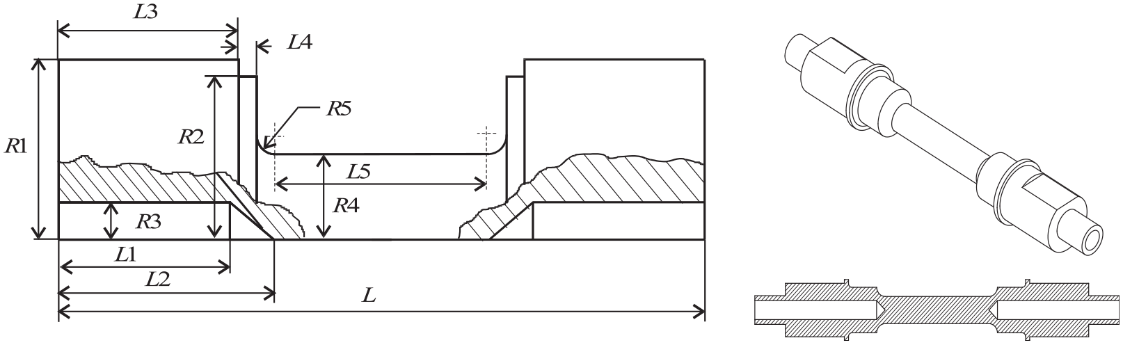
The hollow sample shown in Figure 1 minimizes the radial heterogeneous development of strain and strain rate; however, it is difficult to deform given its thin radial thickness. To partially overcome this problem, Farhoumand et al. ²⁵ modified the sample by adding two thicker hollow shoulders at the sample’s ends and placing two solid and stationary shafts inside the sample while the hollow sample is being twisted. A sample subjected to cold torsion with this technique is shown in Figure 2.

Figure 2.

(a) The geometry of the test sample. (b) the fractured sample after the torsion test.

In another work, Sapanathan et al. ²⁶ employed two longitudinally split solid metallic jackets around the sample to fill the gap between the sample and its induction heating coil. This, shown in Figure 3, makes the heating more uniform and stabilizes the deformation of the hollow sample more by preventing the geometrical instabilities such as those experienced by Farhoumand et al. ²⁵

Figure 3.

Use of split thermal conductors/jackets to improve the heating and to stabilize deformation in a hollow sample.

However, both of these techniques^25,26 add a frictional torque to the recorded data, which has to be taken into account when post-processing the raw data.

The most common specimens used in torsion tests are classified as:

• Those with no cylindrical gauge length ( $L_5=0$ in Figure 4, left), used mainly to investigate the behavior of metals at large strain rates and elevated temperatures, and

• The ones with a cylindrical gauge length, which are mainly used to obtain the strain hardening characteristics.

Figure 4.

Schematic diagram of a specimen of Types I and II for hot torsion test (in a specimen of Type I, $L$ 5 = 0). Left: no clamping ends, Right: with clamping ends.

The design of specimens of Types I and II are shown in Figure 4 left with $L_5=0$ and $L_5\ne 0$ , respectively (the clamping portions are not shown). Figure 4 right shows the clamping portions at both ends of the sample.

The center-holes $R3$ in the sample (Figure 4) are to accommodate thermocouples near the gauge section to monitor and control the heating of the sample.

The test is typically performed in either fixed and free end modes. The latter prevents the length changes but develops axial stress in the sample. The former produces a pure shear deformation. The axial stress development due to the fixed end and the free end (pure shear) are briefly discussed in the next section. In hot torsion tests, torque, twist, time, and temperature are concurrently recorded and the data are reduced to a set of shear-stress shear-deformation curves, each with a constant angular velocity and temperature. Using these raw data, the flow curve is obtained after assuming the yield criterion, commonly von Mises. The test fulfils the second requirement in section 2.2, but the first and third ones can be problematic in some cases.

Compression test

The compression test can produce reasonably homogeneous strain values, which are significantly higher than those of the tension test. The test is conducted in two ways: axisymmetric (ACT) and plane strain (PST).

While the test is mainly used for flow curve identification, it also is used to study texture development and high temperature deformation behavior based on deformation maps (e.g. Rout et al., ²⁷ Dao-chun et al. ²⁸ for ACT, respectively).

The geometry of the compression tests (ACT or PST) is simple enough for analytical purposes. The achievable strains during compression testing of solid or hollow cylindrical specimens are considerably higher than that of the tension test; for example, Hering et al. ²⁹ investigated a typical cold forging steel and showed the maximum strain achieved by tensile test (i.e. the necking stress) was ∼0.12, while a strain of 0.7 was achieved by ACT. Continuous and interrupted uniaxial compression tests were performed by Andrade et al. ³⁰ and Petkovic et al. ³¹ to develop deformation models for steel. The model included microstructural events, such as static and dynamic recrystallization. Moreover, they measured the softening kinetics of static and metadynamic recrystallization by performing interrupted compression tests.

Axisymmetric compression test (ACT)

The ACT is extensively used to design and optimize industrial forming processes. The test characterizes hot and cold flow behaviors of materials and the phenomena associated with them.

The absence of necking, as occurs in a tension test, allows compression test to be conducted to large strains comparable to those of industrial processes such as forging or extrusion; however, barrelling of the specimen, due to friction at the platens, hinders the calculations of the true axial compression stress and from this the identification of the real stress-strain curve of the material. Figure 5 compares undeformed and deformed samples without and with barrelling, respectively. One treatment to prevent barrelling is to apply lubricants, such as PTFE foils ³² ; however, as the sheets of PTFE tear easily, they serve only for a limited range of deformation. Moreover, PTFE may not be safely used at high temperatures, due to the risk of fire. For performing ACT at high temperatures, other options are available; for example, Li et al. ³³ used three different lubricants of molybdenum-disulfide, isopropyl alcohol and acetic acid n-butyl, at their molten state, to reduce friction. To apply these lubricants, the flat ends of the samples are machined with spiral grooves with a depth of ∼0.1 mm (e.g. Tan ³⁴ ).

Figure 5.

Illustration of a compression increment: (a) undeformed-initial sample, (b) barrelling neglected deformed sample described by the cylindrical profile model (CPM), showing an arbitrary cylindrical profile radius ${\overline{R}}_n$ (profile’s effective radius) at an arbitrary time step of $t=t_n$ , and (c) deformed-barrelled sample at $t=t_n$ with an arbitrary barrelled profile’s radius of $R_n\left(z\right)$ .

A recently developed model for ACT (details could be found in Khoddam, ³⁵ Khoddam et al. ³⁶ ) allows the estimation of the test’s heterogeneous deformation and the friction factor via its closed-form solution. Based on a single set of the test’s barrelling-load-deformation data and the model’s closed-form solution, one can estimate the strain and strain rate changes in the sample, instantaneous friction to eventually identify the material’s flow response. To avoid the increase in the friction factor during the test and to compress material homogeneously, the Rastegaev test specimen for ACT ³⁷ (Figure 9) was employed by a few researchers (e.g. Pöhlandt ³⁸ ). However, the unrealistic overestimated strain caused by the sample geometry modification is an important disadvantage of the method. In a purely experimental study, Lovato and Stout ³⁹ performed a large number of compression tests with modified end geometries and lubricants on different materials and recommended the conditions to minimize the barrelling during the test. The suggested procedure, however, does not seem to be transferable to other tests.

Plane strain compression test (PST)

The plane strain compression test (PST) resembles the rolling process more than other tests therefore it is the preferred test method to produce results, particularly texture, comparable with the rolling process. PST is also an important experiment to indirectly measure the flow curves at elevated temperatures. A practice guide for the test through the offices of the National Physical Laboratory (United Kingdom) and the University of Sheffield was suggested. ⁴⁰ Thanks to a reasonably large specimen size that can be utilized in PST, the test is classified as a suitable avenue to study microstructure and texture development during hot deformation. Incremental tests are difficult to perform in a hot PST test for several reasons including the practical problems for lubrication at elevated temperatures. This partly explains why that load-displacement data for hot PST require corrections for the lateral spread and the friction between the platens and the specimen.

Hot plane strain compression is particularly the best option to provide flow curves for modeling plane strain deformation processes, such as rolling. ⁴¹ A typical PST setup and its sample are shown schematically in Figure 6.

Figure 6.

Schematics of PST setup: a sample between upper and lower platens.

Split-Hopkinson pressure bar (SHPB) test

The split-Hopkinson pressure bar, introduced by Bertram Hopkinson, also known as the Kolsky bar, is an apparatus for testing the high strain rate and dynamic stress-strain response of materials. It was known as Hopkinson pressure bar first as it was suggested by Bertram Hopkinson ⁴² to indirectly measure “pulse-like” stress propagation of stress in a metallic bar sample. The test was modified later by Kolsky ⁴³ by utilizing two Hopkinson bars in series, renamed to the split-Hopkinson bar. Incorporating some advancements in the cathode ray oscilloscope in conjunction with electrical condenser units to record the pressure wave propagation in the pressure bars, Kolsky’s modification enabled to indirectly measure both stress and strain and to identify the dynamic flow curve. A design of the Kolsky test (split-Hopkinson pressure bar) can be found in Chen and Song. ⁴⁴ The split-Hopkinson pressure bar will be discussed as a test to characterize ultra-fast deformation and dynamic response of materials that are needed for hot or cold forming processes/events such as explosive forming, ⁴⁵ rod rolling, ⁴⁶ and thermal/cold spray. ⁴⁷

While there are many setups and techniques known as the split-Hopkinson pressure bar, the fundamental principles for these setups and their corresponding measurement are the same. Interestingly, the test is being performed in compression, ⁴⁸ tension, ⁴⁹ and torsion. ⁵⁰ The specimen is secured between the two straight bars, called the incident bar and the transmitted bar, respectively. At the far end of the incident bar, a stress wave is generated to propagate through the bar in the direction of the specimen. This incident wave splits into two smaller waves while reaching the specimen. The first part of the incident wave, known as the transmitted wave, passes through the specimen and into the transmitted bar and is responsible for the plastic deformation of the specimen. The second portion of the wave, known as the reflected wave, bounces back from the specimen and reaches back down the incident bar. ⁵¹ Figure 7 shows an SHPB test setup in compressive deformation mode, its typical mechanical components including a cylindrical sample confined between the incident and transmission bar; the electrical and control subsystems are not shown.

Figure 7.

A schematic of the SHPB test and its sample: a compressive mode.

The tension or compression test setup is usually composed of a long barrel to allow to shape the stabilized with minimum rise time before striking the incident bar. The striker is accelerated by a burst of compressed light gas in a long gun barrel to strike on the end of the incident bar. Several venting holes are devised on the side of the barrel before the exit to allow a non-decelerated strike when colliding the incident bar. The collision velocities are measured carefully, optically or magnetically, just before the collision. Such an accelerating mechanism ensures a controllable and repeatable collision on the incident bar. The striking velocity is reasonably simple to control, for example, by changing the pressure of the compressed gas inside the gun barrel. The loading duration is related to the length of the striker. ⁴⁴ The strain gauges, mounted on the bars, are widely utilized in modern setups to measure strains caused by the propagated waves. Assuming a uniform deformation in the specimen, the stress and strain are calculated based on the amplitudes of the incident, transmitted, and reflected waves.

In the torsional SHPB, a near-perfect square incident wave with a negligible rise time and release time is required. A key subsystem in the torsional test rig is its clamp. A specially designed clamp is usually utilized for this purpose: once the desired torque has been reached between the loading end and the clamp, hydraulic pressure is applied to fracture a notched pin to release the stored torque. Two different designs are shown in Figure 8. Sample designs can be found in Hartmann et al., ⁵² Beattyetal., ⁵³ Chen and Luo. ⁵⁴

Figure 8.

Clamp designs for the torsional Kolsky bar, left: Hartley et al. ⁵⁵ and right: Gilat ⁵⁰ .

Common issues in mechanical testing

The four main mechanical tests reviewed here offer different levels of control to maintain a deformation scenario with fixed effective strain rate and temperature. For example, to prevent variation of strain rate, the test rig applies its load with a controlled rate: a constant angular velocity during torsion test and controlled ram speed for tension and compression tests. These will produce a host of new problems in controlling the homogeneity of the deformation and deformation rate, which are elaborated and discussed in this section.

Comparability of the results from different tests

Each of the major tests reviewed in this article has different capacities to maintain their state of uniaxiality during the entire test and produce different deformation routes such as compression, tension, or shear. To compare the status of deformation in each test sample and to transfer the results to the industrial processes, the samples’ effective stresses are compared together which are bound by the definition of the yield surface and criteria. It is very likely that the effective stress in each sample, measured at the physical simulation bench scale, is different from that of the other test and that of the industrial forming processes.

Known issues with tension test

To keep the strain rate constant in the tension sample, a variable ram speed control is needed. Upon the onset of necking, the ram speed control can no longer maintain a uniform effective strain or strain rate within the sample or to that planned strain rate for the entire deformation range.

Performing the tensile test at elevated temperatures reduces the usefulness of the test further as it introduces several new issues. The shortrange of uniform deformation ⁵⁷ and the occurrence of a too early triaxiality ⁵⁸ are two main issues that extremely complicate the post-processing of the raw data.

While there are a few numerical solutions for the hot tension test (e.g. Lombard et al. ⁵⁹ ), closed-form solutions are only available for the pre-necking. ⁶⁰ The latter does not enable indirect stress measurement post necking. Consequently, the (hot) tension test is not a preferred avenue to characterize the plastic behavior of materials or to physically simulate hot deformation processes.

Known issues with hot torsion test

One of the known issues with the hot torsion test is the radial variation of the strain and strain rate; therefore, both effective strain and strain rate of a material point in the test sample change linearly with their distance from the axis of rotation. The constant angular velocity results in heterogeneous deformation and deformation rate in the sample. The effective strain and strain rate of a material point in the sample increases radially and proportionally with the point’s distance from the sample’s longitudinal axis, and the values change linearly from zero at the sample’s centerline to their maxima at the sample’s outer surface. The strain rate at each radius remains constant during the test, while the effective strain accumulates with twist angle.

Deformation outside the gauge section may introduce some errors in the obtained flow stress. This is particularly the case for the test subjected to high strains, strain rates, and high temperatures. Grabianowski and Kurowski ⁶¹ compared the distribution of hardness on a cross-section of the hot torsion specimen before and after the test as an indication of deformation (work hardening). They noticed that the hardness of the zone outside the measured area of the hot torsion test specimen had changed. They concluded then that the specimen had deformed outside the gauge section. To account for the deformation occurring outside the gauge section, one requires to employ an effective gauge length that changes with deformation. Pöhlandt et al. ⁶² proposed a semi-empirical method to account for deformation outside the gauge section. They proposed a formula to account for deformation outside the gauge section. It involves the calculation of an effective length to be used in the analytical methods for the reduction of the torque-twist data into the flow data. The formula was based on a power-law constitutive equation and required instantaneous effective length which limited its applicability. Later, the method was modified ⁶³ to employ more general constitutive equations.

Another critical issue is that the sample deforms in pure shear, which does not resemble many real industrial processes.

Length changes during high torsional strains

On the suggestion of Nadai, ⁶⁴ MacGregor measured the length of a round bar of soft copper after it had been twisted near the fracture torque and found a small permanent increase of length in the twisted copper cylinder. Also, Davis ⁶⁵ took Vickers hardness readings along a radius in the cross-section of a round bar of copper after it had been severely twisted and cut in pieces. He found work hardening at the center of the circular cross-section in the axis of the bar. These observations indicated that the center portion of a cylinder of originally soft ductile metal after it was severely permanently twisted, is permanently strained in the axial direction. It was concluded by Davis that the distribution of shearing stress $\tau =f(r,\theta )$ did not represent the complete system of stresses in round bars after a considerable torsional overstrain and a system of secondary normal stresses in axial and possibly also in radial and tangential direction must be present in addition to the distribution of shearing stresses $\tau =f(r,\theta )$ deforming the metal.

Swift first stated that in free end torsion tests of mild steel, significant changes in length occur with increasing strain. Swift ⁶⁶ effect is a result of texture development in the sample and develops longitudinal stress in the sample. The causes of the axial deformation are still uncertain, though it has been suggested that they were probably related to anisotropy and texture development in the specimens (e.g. see Tóth et al. ⁶⁷ ) or due to higher-order terms in strain (Ronay ⁶⁸ ). According to Hodierne, ⁶⁹ if the ends are free, corrections may be made for the changes in specimen dimensions.

More commonly, specimens are axially constrained (see Figure 4) so that specimen geometry remains constant, but axial stresses are developed. The conversion of torque ( $M$ ) to surface shear stress ( $\tau$ ) for this case was simplified by Fields and Backofen. ⁷⁰

There is evidence from the studies of solid and tubular specimens of different geometry that the radial dependence of stress developed due to constraining the end of the torsion test specimen is small such that the average axial stress ( ${\sigma }_{\mathrm{A}}$ ) can meaningfully be obtained. According to Sellars and Tegart ⁷¹ :

$$\sigma =(3{\tau }^2+{\sigma }_{\mathrm{A}}^2{)}^{\frac{1}{2}}$$

(1)

the longitudinal stress may generally be neglected without introducing significant errors in the derivation of the effective stress, using the von Mises criterion.

Known issues with the compression test

While the compression test is regarded as the most versatile test for workability, it suffers from critical issues, as summarized in the introduction, regarding friction, temperature, and strain-rate control. These could be minimized by proper test equipment and experimental planning when performing the test at elevated temperatures.

Barrelling

To identify the material flow stress to account for the barrelled shape of the deformed sample, Chen and Chen ⁷² extended Hill’s general solution of the compression test and obtained identical expressions for effective strain and strain rate to those obtained by Avitzur. ⁷³ These were unable to estimate the shearing strain/rates and their contribution to the effective stress and strain.

Correction factor

Ettouney and Hardt ⁷⁴ derived a bulge correction factor to find effective stress by accounting for the barrelling. The factor was based on Bridgman’s correction factor for effective stress after necking in the tensile test ⁷⁵ and was applied to the calculated ideal flow stress assuming no friction. The approach offered no correction factor for strain or strain rate in the sample. This could be a major disadvantage for microstructural studies and the correlation of the structure with deformation and deformation rate.

Evans and Scharning ⁷⁶ demonstrated numerically that the test produces systematic errors in its identified flow curve. They also concluded that due to sufficiently similar internal properties of many alloys under hot working conditions, it is justified to generalize the trends obtained by the numerical studies (e.g. the pattern of deformation heterogeneity in the sample). They found that friction and geometry play the most important role in the heterogeneities with strain and strain rate playing an intermediate important role, while the temperature can be marked as low importance. Similar conclusions were made by Fardi et al. ⁷⁷

Handling of friction

One of the disadvantages of compression tests is the presence of friction at the interfaces of the specimen and the compression plates. It has been reported that the friction is not constant and increases with the test; for example, see the experimental findings by Han ⁷⁸ for the ACT and by Wang and Ramaekers ⁷⁹ for the PST. Despite attempts to minimize barrelling during ACT, it cannot be fully eliminated. This is more challenging if large reductions are required to characterize the material’s flow behavior with higher plastic strains.

While friction can be highly reduced for testing soft materials, for example, polymers and biological tissues, using solid, liquid, or gaseous lubricants, ⁸⁰ it cannot be fully removed for testing metallic samples with a useful large deformation. Moreover, the difficulty in directly measuring friction hinders its accurate modeling; therefore, friction becomes a source of uncertainty in establishing a constitutive model based on the compression test results.

Several methods have been proposed to minimize the friction, such as the use of mica or thin metallic shims of softer materials at the tool-sample interface or modifying the interfaces (known as Rastegaev ⁸¹ lubrication). A schematic of Rastegaev ⁸¹ sample with two recesses at its interfaces with the platens is shown in Figure 9.

Figure 9.

Rastegaev sample: two recesses are filled with a proper lubricant before the test to minimize friction.

These recesses are filled with a proper lubricant before performing the test to minimize friction. Unfortunately, the good lubrication in the Rastegaev tests has a serious backlash; it increases the error of height measurement: the measured reduction of height and sample’s effective strain and strain rate are influenced by deformation of the recesses. A detailed study on the error as a function of the recess and sample geometry can be found in Pöhlandt. ³⁸

The friction, responsible for barrelling, makes the analysis and interpretation of the test results extremely difficult. The use of ring compression to estimate the friction coefficient is questionable; it employs an extrapolation method that serves to eliminate friction after-testing evaluation. At least two or three extra tests, resembling the real test, are required to correlate the findings to the real tests. Furthermore, the extrapolation can be inaccurate because of the inhomogeneous deformation of the specimens.

Another complication is that the friction factor is not constant and changes with the sample’s geometry during the test. To overcome this problem, researchers have proposed different approaches. For example, Cook and Larke ⁸² developed a way to account for the frictional losses. They estimated the zero-friction flow strength by extrapolating the results of the test for different height-to-diameter ratios. This may be an approach to account for frictional losses during a given testing condition, but it is not sufficient in general for removing the uncertainty caused by friction and obtaining an accurate constitutive equation. Alternatively, Pöhlandt and Roll ⁸³ suggested a new specimen geometry to overcome the difficulty with frictional losses. The new specimen is composed of two trapezoid shoulders connecting to the gauge section of the compression test specimen. The errors due to neglect of stress and strain concentration at the conjunction of the shoulders to the gauge section can be considerably higher than that due to neglect or inappropriate modeling of friction. ³⁸

Other methods to overcome the friction issue include modification of sample geometry or tool-sample interface and discontinuous tests which might be useful for limited test scenarios.

Li and Ma ⁸⁴ developed a mathematical model to account for friction when identifying the flow behavior of material using the test; however, the friction factor calculation method used in this work ⁸⁵ has proved to be inaccurate and unreliable; see, for example, Fardi et al., ⁷⁷ Solhjoo, ⁸⁶ Khoddam and Hodgson. ⁸⁷

Based on some thermal-mechanical numerical simulations, Evans and Scharning ⁷⁶ suggested a way of estimating the friction during the ACT and correcting the flow curve obtained from the test; however, his results were based on several limiting assumptions including a simple power-law constitutive equation and therefore their findings are not transferable to a general test.

Li et al. ³³ proposed a method to evaluate the friction coefficient in ACT based on a combined approach. The method relies on simulation of the test and the Avitzur barrelling model ⁷³ and calculation of its barrelling parameter based on the method of Ebrahimi and Najafizadeh ⁸⁵ ; however, the latter has been shown to have serious limitations.^86,88

Another approach is to indirectly characterize/measure friction using the barrelled sample geometry, for example, Alexandrov et al., ⁸⁹ Yao et al., ⁹⁰ Fan et al., ⁹¹ and Solhjoo and Khoddam. ⁸⁸ Methods to account for friction, excluding the barrelling, with either a fixed Coulomb friction coefficient and mixed sticking-sliding friction, as well as a recently developed method by Khoddam et al. ³⁶ are reviewed and discussed in section 6.

Inhomogeneous deformation during compression, advantage or disadvantage?

The compression test is favored less compared to the hot torsion test due to its limitation to provide high effective strains (see for example Khoddam et al. ⁹² ). Also, numerous workers have reported that the flow stresses identified by the hot torsion test are lower than those obtained by axisymmetric tension and compression tests. ⁹³ The latter could be due to the different modes of deformation in each test, that is, shear, tensile, and compressive.

Barrelling adds extra complications for the interpretation of the test data as a result of a subsequent inhomogeneous state of deformation in the test sample; however, the inhomogeneous deformation could be beneficial upon the availability of a reliable model for its analysis. The first benefit is that a multi-axial deformation represents industrial forming processes more realistically. The second advantage is that the maximum effective strain in a heterogeneously deformed compression sample overarches a wider range of deformation with a significantly higher effective strain compared to its homogeneously deformed counterpart. ³⁵

A systematic numerical study of the test was conducted by Ye et al. ⁹⁴ to assess the heterogeneity of deformation during the test. Also, they highlighted the error in correlating the microstructural observations at the sample center to the strain and strain rate estimated based on the available solutions of the test. The study is limited to case studies of the heterogeneous deformation without a recommendation to minimize it or how-to post-process the test data to account for the heterogeneity.

Foldover

Foldover is a complex transient boundary condition in several forming processes including the barrelling compression test (BCT). Foldover in compression test may be compared with triaxiality and necking during the tensile test. The significance of foldover on the interpretation of the test data has been ignored in the current literature; the onset of foldover during BCT is comparable to that of necking in the tensile test. Foldover increases with friction and deformation and is practically inevitable in many forming scenarios. However, methods to detect its onset and to measure its growth during the test are not adequately detailed to allow the separation of the pre- and post-foldover raw data.

Rams speed induced inhomogeneous strain rate

Ram speed control contributes further to the variations of the strain rate as a function of time; this is apart from effective strain rate inhomogeneities induced by barrelling in the sample. A constant crosshead speed ACT does not produce a constant strain rate during the test. Also, it is not possible to keep the strain rate constant over the entire sample by simply varying the cross-head speed. As a result, a distortion of the flow curve occurs because of strain-rate sensitivity.

The issue of strain rate changes during the test or process and its interaction with the results are discussed by Abbod et al. ⁹⁵ It has a big bearing on the reliability of the identified flow curves.

Given a kinematic model that accounts for barrelling, the ram speed, effective strain rate and strain distribution in the sample can be correlated (e.g. Khoddam, ³⁵ Khoddam and Hodgson ⁸⁷ ). The model can be used in the experimental setup to control the ram speed as a function of the sample’s instantaneous height to minimize the heterogeneous strain rate changes in the sample in an average sense. More details on this issue can be found in section 6 of this article.

Ultra-high strain rate and deformation heat

ACT-based high strain rate simulations pose a host of new issues, which eventually worsen the heterogeneity. ⁹⁶ One problem normally encountered with high strain rate testing is the inertia of the moving ram. Many computer-controlled systems will have problems starting or stopping the test on time. The above problem can be overcome using a momentum trap or brake similar to that used in SHPB. ⁴⁴ For example, the TMTS machine uses a wedge, which acts as a stopping mechanism to counteract this problem. The position of the wedge is calculated from the initial height of the specimen and the desired strain level.

Figure 10 shows a strain rate versus time plot for a high strain rate AST test. The figure illustrates a major advantage of using this system for such tests. The travel of the ram allows the tools to already be at speed when they first come into contact with the sample, meaning that the desired strain rate is experienced from the start to the end of the test. The sudden drop-off in strain rate at the end of the test is caused by the ram coming into contact with the wedge mechanism.

Figure 10.

TMTS strain rate versus time plot. ³

The developed constitutive model is more credible when the measured data range is similar to those of the process. Split-Hopkinson bar and torsion tests can be used to obtain the constitutive raw data at high strain rates and high strains, respectively. Alternatively, a non-ideal remedy to this problem is to scale up the results with creep and the similarity theory in mind; see, for example, Khoddam et al. ⁹⁷ and Zener-Holloman parameter. ⁹⁸

Representative point

Upon availability of a kinematic model for ACT which accounts for barrelling, a point in the sample can be chosen as the representative point for flow curve identification that can provide effective strains comparable to those achievable by the hot torsion test (see section 6 of this review). EPM theory of ACT allows tracing flow stress at different points. Given the heterogeneity of EPM’s solution, these flow curves have different maximum stress, strain, and strain rates. A representative point should be defined/chosen in the sample at which the flow is traced. Using the EPM solution of ACT, the effective stress, strain, and strain rate are evaluated at this point to convert the existing experimental data to the flow curve. This will allow the inclusion of the sample’s maximum formability and effective strain during the test and eventually in the flow curve; the flow curve is followed along with the representative point.

Known issues with Split-Hopkinson pressure bar (SHPB) test (Kolsky test)

Primary concerns for valid SHPB experiments have been focused on specimen design, force sensing, and pulse shaping design to achieve uniform deformation/stress equilibration and constant strain rate deformation in the specimen. Contrary to other traditional flow stress tests, there is no standard or commonly used procedure currently available to convert the measured raw high rates data to the flow curves; therefore, discrepancies exist in the results reported by different research groups, with different samples.

Constant strain rate and a need for pulse shaping

Keeping the strain rate over the entire test duration constant is generally a challenging experimental issue. This is particularly the case with an SHPB test given its super high strain rates. A suitable “pulse shaping” technique/system is carefully devised and implemented to change the waveform induced/transmitted in the sample by the incident bar (see Figure 7). This is to ensure that the inevitable stabilizing lag associated with the desired wave has a minimal impact on the speed changes of the incident bar during the sample. It usually requires a long distance between the “air gun” and the sample to be traveled by the incident bar before hitting the sample to start the wave and before hitting the momentum trap to stop the wave. This brings a whole new set of issues such as a need to utilize laser devices to carefully align the Teflon bearing used to guide the incident bar bars.

The Split-Hopkinson pressure bar test provides constitutive raw data suitable for a typical ultra-high strain rate process. However, the provision of meaningful high strain rate data during a test is limited by the dynamic response time of the actuators used in the closed-loop circuit of the test rig. For example, to create a strain rate of $2000s^{-1}$ during a typical torsion test that is running at 3300 rpm with a response time of $0.015\mathrm{s}$ , approximately two full specimen revolutions are necessary before the velocity stabilization. The currently available technology can not provide the required ultra-fast stabilization. Therefore, the credibility of a high strain rate constitutive model established upon such data is not automatically guaranteed.

Shared limitations of SHPB with other tests

Depending on the mode of the SHPB test (e.g. tensile, compressive, or torsional), all post-processing limitations mentioned with other mechanical tests in this section are generally present in the SHPB as well. These limitations and issues are not repeated here for the sake of brevity.

Deformation heat

Strain rate is responsible to develop deformation heat in sample. ⁹⁹ Methods to evaluate the temperature rise during the test are discussed and presented in Sasso et al. ¹⁰⁰ : the heat complicates temperature control during the test.

Heterogeneous deformation in the sample

The dynamic test is being performed on three different modes which are tensile, compressive, and torsional. The experimental setups are quite diverse in their design and their employed theory. This complicates the already difficult comparison of the results.

Similar to other mechanical tests, it is practically very challenging to eliminate or minimize the heterogeneity of deformation, deformation rate, or temperature in its deforming sample (see, for example, Sasso et al., ¹⁰¹ Kariem et al. ¹⁰² ).

Currently used post-processing methods

These methods are typically the simplest ones, making them preferred by the researchers due to their ease of use. Therefore, it is most likely that some of the issues outlined in the previous section have not been addressed in these simple methods.

Tension test

This test has been rarely used for hot flow curve identification as it can produce strains much lower than those occurring in the industrial forming processes. The test has been included in this review for the sake of completeness. The interested reader can find example usage of the test for flow curve identification in Dieter, ¹⁰³ Dieter et al. ¹⁰⁴ Also, reference Pöhlandt ³⁸ can be studied for details on the approximative determination of flow curves from characteristic values obtained by tensile tests.

Hot torsion test

Existing analytical work on the hot torsion in the literature may be either divided into direct closed-form analytical solutions and numerical solutions of the hot torsion test, or into inverse solutions. The direct closed-form solutions are referred to as analytical solutions in this context, which in turn may be divided into four groups:

1. Elastic solutions of pure torsion,

2. Plastic solutions of pure torsion,

3. Reduction of torque-twist data to shearing stress and strain, and

4. Length changes during the torsion test.

In the current literature, both analytical and numerical solutions of the hot torsion test have been used directly or inversely. While a closed-form direct solution is always based on many simplifications, but if modified, it can provide a proper initial guess for the complex inverse numerical solutions (e.g. Khoddam et al., ²⁰ Gelin and Ghouati ¹⁰⁵ ).

Kinematics of the torsion test

It is assumed that the gauge section of a tubular torsion test specimen can be represented as shown in Figure 1, twisted by a torque $M$ acting around its axis.

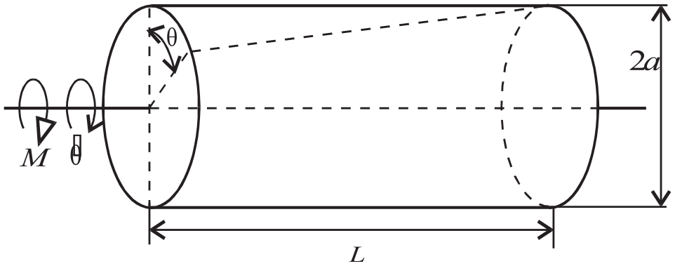
The kinematic model is generally the first theoretical layer for many boundary value problems including the torsion test. This test has simple kinematics as shown in Figure 11. The illustration shows the gauge section of a torsion sample and the radius dependent nature of the plastic strain in the sample twisted by a twist angle of $\theta$ . Upon the movement of the material points in the torsion sample due to pure torsion (fixed end), the sample deforms. Due to the linear increase of the effective strain with radius (i.e. $\epsilon \propto r$ in Figure 11(c)), the effective strain and strain rate increase linearly in the radial direction. This is because the velocity field in the gauge section of the deforming torsion sample is one-dimensional (tangential). The only velocity component is the tangential velocity $V_r$ :

$$V_{\theta }=\frac{\mathrm{rz}\stackrel{·}{\theta }}{l},0<r<r_o,V_z=0,V_r=0$$

(2)

Figure 11.

Torsion sample (a): undeformed, (b): deformed by a twist angle of $\theta$ , and (c): the distribution of effective strain as a function of the radius in the radial and longitudinal directions.

It can be concluded that:

$${\stackrel{·}{\epsilon }}_{\mathrm{zz}}={\stackrel{·}{\epsilon }}_{\mathrm{rr}}={\stackrel{·}{\epsilon }}_{\theta \theta }={\stackrel{·}{\epsilon }}_{\mathrm{rz}}={\stackrel{·}{\epsilon }}_{r\theta }=0$$

(3)

The only non-zero component of strain rate in the sample, shearing, can be found as:

$${\stackrel{·}{\epsilon }}_{z\theta }=\frac{1}{2}(\frac{\partial V_{\theta }}{\partial z}+\frac{1}{r}\frac{\partial {\mathrm{V}}_{\mathrm{r}}}{\partial \theta })=\frac{1}{2}\left(\frac{r\stackrel{·}{\theta }}{l}\right)$$

(4)

where $l$ and $r$ are the sample length and radial coordinate of the deformation point, respectively. The shear strain and shear strain rate at a radial distance, $r$ , are:

$${\gamma }_{z\theta }=2{\epsilon }_{z\theta }=\frac{r\theta }{l},{\stackrel{·}{\gamma }}_{z\theta }=2{\stackrel{·}{\epsilon }}_{z\theta }=\frac{r\stackrel{·}{\theta }}{l}$$

(5)

Assuming that the material is isotropic, the von Mises effective strain rate in the sample becomes:

$$\stackrel{.}{\overline{\epsilon }}=\sqrt{\frac{2}{3}{\stackrel{.}{\epsilon }}_{ij}.{\stackrel{.}{\epsilon }}_{ij}}=\sqrt{\frac{2}{3}\left({\stackrel{.}{\epsilon }}_{rr}^2+{\stackrel{.}{\epsilon }}_{\theta \theta }^2+{\stackrel{.}{\epsilon }}_{zz}^2+\frac{1}{2}\left({\stackrel{.}{\gamma }}_{rz}^2+{\stackrel{.}{\gamma }}_{z\theta }^2+{\stackrel{.}{\gamma }}_{r\theta }^2\right)\right)}$$

(6)

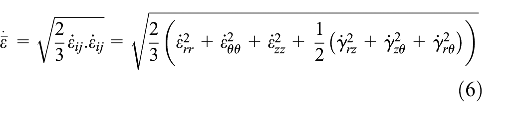
which can be simplified as:

$$\stackrel{.}{\overline{\epsilon }}=\frac{r\stackrel{·}{\theta }}{\sqrt{3}l}$$

(7)

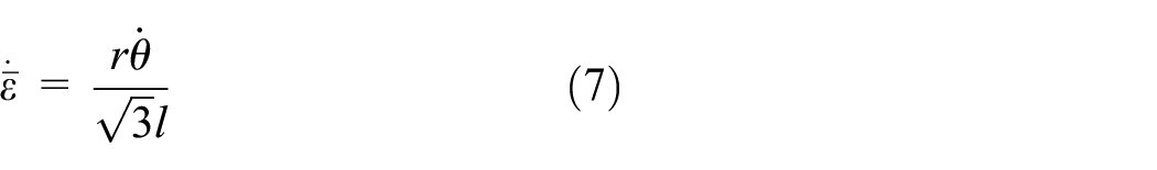
For pure torsion, the von Mises effective strain, $\overline{\epsilon }$ , becomes $\overline{\epsilon }={\gamma }_{z\theta }/\sqrt{3}$ .

Equation (7) is graphically shown in Figure 11; the velocity field and its resulted effective strain and strain rate at a given radius, $r$ , and their maximum values at the outer radius, $r_O$ , are shown in Figure 11(c).

Analysis of elastic torsion

Closed-form solutions for torsion analysis exist for shafts with only the simplest geometry. The Ritz technique has been used together with the theorem of minimum potential or complementary energy for obtaining approximate solutions for shafts of more complex geometry; however, this method is difficult for shafts with complicated cross-sections. A suitable series of functions that approximates the dependent variable must be found for each cross-sectional shape. It is more desirable to find a solution that is equally applicable to all shafts regardless of their cross-sectional configuration. We restrict ourselves here to the case of axisymmetric shafts used in hot torsion tests.

The solution of the elastic torsion of bars by couples applied at the ends was given by Saint-Venant. ¹⁰⁶ He used the so-called Semi-inverse method. Certain assumptions were made about the deformation of the twisted bar and he showed that with these assumptions he could satisfy the equilibrium equations and the boundary conditions. From the uniqueness of the solutions of the elasticity equations (Timoshenko and Goodier ¹⁰⁷ ), it follows that the assumptions were correct and the solution obtained was the exact solution of the torsion problem.

To demonstrate the solution, let us consider a circular shaft of variable diameter as shown in Figure 12. The axis of the shaft is taken as the $z$ axis and the polar coordinates $r$ and $\theta$ are used to define the position of an element in the plane of a cross-section. The stress components are ${\sigma }_r$ , ${\sigma }_{\theta }$ , ${\sigma }_z$ , ${\tau }_{\mathrm{rz}}$ , ${\tau }_{r\theta }$ , and ${\tau }_{z\theta }$ . If the components of displacement in the radial, tangential, and $z$ directions are denoted by $u$ , $v$ , and $w$ respectively, the exact solution satisfies the following equation (see e.g. Timoshenko and Goodier ¹⁰⁷ ):

$$\frac{{\partial }^2\varphi }{\partial r^2}-\frac{3}{r}\frac{\partial \varphi }{\partial r}+\frac{{\partial }^2\varphi }{\partial z^2}=0$$

(8)

Figure 12.

Pure torsion of a circular shaft of variable diameter.

where $\varphi$ is an elastic stress function of $r$ and $z$ such that:

$$r^2{\tau }_{r\theta }=-\frac{\partial \varphi }{\partial z}ãr^2{\tau }_{z\theta }=\frac{\partial \varphi }{\partial r}$$

(9)

The boundary conditions for the function $\varphi$ are:

$$\frac{\partial \varphi }{\partial r}\frac{\mathrm{dr}}{\mathrm{ds}}+\frac{\partial \varphi }{\partial z}\frac{\mathrm{dz}}{\mathrm{ds}}=0$$

(10)

in which $\mathrm{ds}$ is an element of the boundary.

Analysis of plastic torsion with no hardening

The components of ${\tau }_{r\theta }$ and ${\tau }_{z\theta }$ are the only non-vanishing components of stress. At a certain point of the cross-section at which yielding occurred, both shear stress components ${\tau }_{r\theta }$ and ${\tau }_{z\theta }$ must satisfy the condition of plasticity:

$${\tau }_{r\theta }^2+{\tau }_{z\theta }^2=k^2$$

(11)

The constant $k$ is the yield stress in pure shear. It is equal to ${\sigma }_0/2$ for Tresca yield criterion, and equal to ${\sigma }_0/\sqrt{3}$ for von Mises yield criterion, where ${\sigma }_0$ is the uniaxial yield stress in tension.

Two of the three equations of equilibrium are identically satisfied automatically while the third reduces to:

$$\frac{\partial }{\partial r}\left(r^2{\tau }_{r\theta }\right)+\frac{\partial }{\partial z}\left(r^2{\tau }_{\theta z}\right)=0$$

(12)

Equation (12) is satisfied if ${\tau }_{r\theta }$ and ${\tau }_{z\theta }$ are derived from a stress function $\zeta (r,z,\alpha )$ such that:

$${\tau }_{r\theta }=\frac{k}{r^2}\frac{\partial \zeta }{\partial z}\mathrm{and}{\tau }_{\theta z}=\frac{k}{r^2}\frac{\partial \zeta }{\partial r}$$

(13)

where $\alpha$ is the relative angle of twist of one end of the shaft relative to the other end.

If the stress components from equation (13) are substituted into equation (12), the following equation will be obtained:

$${\left(\frac{\partial \zeta }{\partial r}\right)}^2+{\left(\frac{\partial \zeta }{\partial z}\right)}^2=r^4$$

(14)

There is no closed-form solution for equation (14). A numerical method however can be used to solve the governing equation (14) for the stress function. Nadai ¹⁰⁸ used the sand-heap analogy to show the distribution of $\zeta$ within the cross section.

Reduction of torque-twist data

In the determination of the flow stress/constitutive parameters from the hot torsion results, the shear stress should be calculated. A schematic diagram of the cylindrical part of the hot torsion test specimen is shown in Figure 13.

Figure 13.

Schematics of the cylindrical part of the hot torsion test specimen.

The first step, and the most difficult one in the reduction of the torque twist data, is to extract shearing stress from the integral $M=2\pi {\int }_0^a\tau r^2\mathrm{dr}$ . Depending on the choice of the constitutive equation, there may be no closed-form solution for this integral. Four of the most important techniques for the reduction of the torque-twist data; the differential, Nadai, Fields and Backofen, and Semiatin’s method will be reviewed here.

The differential method

The results obtained from two tests, at the same twist rate with samples of radii $a_1$ and $a_2$ close together, are required to use this method (Cook ¹⁰⁹ ). For a given twist, $\theta$ , the differences in torque may be expressed as:

$$M_2-M_1=2\pi {\int }_{a1}^{a2}\tau r^2\mathrm{dr}$$

(15)

The major assumption made in this technique is that the shear stress is nearly constant and equal to $\overline{\tau }$ in the thin layer between $a_1$ and $a_2$ . Equation (15) can be rewritten as:

$$M_2-M_1=2\pi \overline{\tau }\left(\frac{a_2^3-a_1^3}{3}\right)$$

(16)

from which the average shear stress $\overline{\tau }$ can be calculated:

$$\overline{\tau }=\frac{3\pi }{2}\left(\frac{M_2-M_1}{a_2^3-a_1^3}\right)$$

(17)

The corresponding shearing strain with $\overline{\tau }$ is

$$\overline{\gamma }=\frac{(a_1+a_2)\theta }{2L}$$

(18)

The advantage of this method is that it applies to materials obeying any kind of constitutive law; however, it is difficult to obtain the same initial condition for both specimens, especially the initial thermal and microstructural conditions.

Nadai’s method

Nadia’s ¹⁰⁸ surface stress method required sophisticated data analysis since the shear stress is nonlinearly distributed along the radius of a solid circular bar. An iterative procedure was required to determine the stress in this method. Also, in this method, it was assumed that the shearing stress was independent of the shearing strain rate.

A full plastic method (thin-walled tube approximation) was presented by Brown. ¹¹⁰ In this method, it was assumed that the shear stress was uniformly distributed across the wall thickness. The shear stress-strain curve obtained by this method was lower than the curve obtained by torsion or compression tests.

Batdorf and Ko ¹¹¹ used a quasi-elastic (QE) approximation, which is equivalent to assuming a linear shear stress distribution in the specimen with respect to the radius and finding the shear stress-strain relation at the surface of the specimen. Their method overestimated the shear stress at a given strain and gave an upper bound to the shear stress-strain curves.

To examine the basic concepts of Nadai’s surface stress method, let us consider the torque twist data as shown in Figure 14, where ${\theta }^{\prime }=\frac{\theta }{L}=\frac{\gamma }{r}$ is twist per unit length of the specimen. It is assumed that $\tau =f\left(\gamma \right)$ is not necessarily a power-law constitutive equation. It can be shown that (Nadai ¹⁰⁸ ):

$${\tau }_a=f\left({\gamma }_a\right)=\frac{1}{2\pi a^3}·\frac{1}{{\theta }^{\prime 2}}\frac{d}{d{\theta }^{\prime }}\left(M{\theta }^{\prime 3}\right)$$

(19)

Figure 14.

Torque-twist curve.

where $a$ is the outer radius of the specimen. By drawing the tangent to the torque-twist curve (Figure 14) at a few points, ${\tau }_a$ for various values of ${\gamma }_a$ (i.e. a function ${\tau }_a=f({\gamma }_a))$ can be calculated by measuring the length of the two straight lines $\overline{\mathrm{CP}}$ and $\overline{\mathrm{AP}}$ via ${\tau }_a=\frac{1}{2\pi a^3}(\overline{\mathrm{CP}}+3\overline{\mathrm{AP}})$ .

Nadai’s surface stress method does not take into account the dependence of shear stress on the shear strain rate; therefore, for the hot torsion test under high strain and strain rates, where shear stress highly depends on shear strain rate, Nadi’s surface stress method leads to serious error. Furthermore, use of the slope of the $M$ versus ${\theta }^{\prime }$ the curve can introduce more errors, due to the existence of experimental noise.

Fields and Backofen’s method

Fields and Backofen ⁷⁰ have extended Nadai’s method to rate-sensitive materials. They obtained a relationship between shearing stress, torque and twist similar to equation (19):

$${\tau }_a=\frac{1}{2\pi a^3}(\theta \frac{d{M}_{\mathrm{c}}}{d\theta }+3M_{\mathrm{c}})$$

(20)

The value of “constructed torque” $M_{\mathrm{c}}$ , however, is different from the value of torque $M$ in equation (19). The constructed torque-twist curve should satisfy a condition under which:

$$\frac{{\stackrel{·}{\theta }}_1}{{\theta }_1}=\frac{{\stackrel{·}{\theta }}_2}{{\theta }_2}=\frac{{\stackrel{·}{\theta }}_3}{{\theta }_3}=\cdots =\frac{{\stackrel{·}{\theta }}_a}{{\theta }_a}$$

(21)

This condition has been shown in Figure 15. Fields and Backofen showed that equation (20) can be written in the following form:

$${\tau }_a=\frac{M}{2\pi a^3}(n+m+3)$$

(22)

Figure 15.

Construction of a Torque-Twist curve for which $\frac{\stackrel{·}{\theta }}{\theta }=\frac{{\stackrel{·}{\theta }}_a}{{\theta }_a}$ from torque-twist records at constant twist rates (Fields and Backofen ⁷⁰ ).

in which:

$$n={\left(\frac{\partial \ln M}{\partial \ln \theta }\right)}_{\stackrel{·}{\theta }}\mathrm{and}m={\left(\frac{\partial \ln M}{\partial \ln \stackrel{·}{\theta }}\right)}_{\theta }$$

(23)

where $n$ and $m$ are two important constitutive parameters called the strain hardening and strain rate sensitivity indexes respectively.

One advantage of Fields and Backofen’s method is that it can be used with any form of the rate-sensitive constitutive equation. The major limitation of this method is that the torque is assumed to be a unique function of the amount of twist and twist rate $\stackrel{·}{\theta }$ with no regard to the history of the test. This is a major disadvantage when performing interrupted tests to simulate multi-pass rolling or when the material exhibits multiple regimes of hardening. ¹¹² The labor involved to obtain the constructed torque $M_c$ from the available torque twist data is considered as another disadvantage of this method. The method considers the shearing stress at the surface which can produce more error due to surface imperfections such as micro cracks and scale due to high temperature of the specimen. An extension of this method was presented in Khoddam and Hodgson ¹¹² which accounts for materials with multiple regimes of hardening.

Semiatin and Halbrook’s method

For some special forms of the constitutive equation, the integral equation $M=2\pi {\int }_0\tau r^2\mathrm{dr}$ can be solved analytically to obtain a closed-form solution for the reduction of the torque-twist data. Semiatin and Holbrook ¹¹³ obtained a torque-twist equation of similar form to that of Fields and Backofen (equation (22)) provided that a simple power-law equation of the following type is assumed:

$$\tau =G{\gamma }^n{\stackrel{·}{\gamma }}^m$$

(24)

In this method, the simple torque-twist data can be used and the data do not need to satisfy equation (21). This method is limited as it cannot accommodate a recovery or recrystallization type softening in its flow curve.

Axisymmetric compression test

Two main types of post-processing methods for the ACT involve (1) exclusion of barrelling and (2) inclusion of barrelling ³⁸ ; the latter is considered as an advanced method and will be reviewed later in section 6 of this article.

Kinematic solutions of compression test

Consarnau and Whisler ¹¹⁴ proposed a deformation velocity field to identify material flow behavior during the compression test. Their method relies on the conservation of momentum and mass with friction contact surfaces to account for the barrelling and heterogeneous deformation; however, their use of many simplifying assumptions to model and solve the governing equations limit the transferability of their derivations in the real deformation scenarios.

To describe a general kinematic model for the ACT, a material point in the deforming sample is considered whose velocity vector, $\overrightarrow{\phi }$ , is of the following form:

$$\overrightarrow{\phi }=\stackrel{·}{u}\overrightarrow{e_r}+\stackrel{·}{w}\overrightarrow{e_{\theta }}+\stackrel{·}{v}\overrightarrow{e_z}$$

(25)

with $\overrightarrow{e_r}$ , $\overrightarrow{e_{\theta }}$ , and $\overrightarrow{e_z}$ as the unit vectors in radial, tangential, and axial directions, respectively (Figure 5). Also $u\prime$ , $w\prime$ , and $v\prime$ denote the magnitude of the radial, tangential, and axial components of displacements, respectively, and the superscript dot shows their corresponding time derivatives (velocities). In Figure 5 the no-barrelling velocity fields and those of the barrelled sample have been distinguished using superscript prime.

In the conventional cylindrical profile model of ACT (no-barrelling), the following simple kinematic descriptions with a bi-linear velocity field are used:

$$\stackrel{.}{u^{\prime }}\left(r\right)=\frac{\stackrel{.}{\overline{R}}r}{\overline{R}}=-\frac{r\stackrel{·}{H}}{2H},\stackrel{·}{v}\prime \left(z\right)=\frac{z\stackrel{·}{H}}{H},\stackrel{.}{w\prime }=0$$

(26)

where $\overline{R}=0.5D_0\sqrt{H_0/H}$ is the sample’s effective/equivalent profile radius (Figure 5(c)). Using definitions of strain rate components for the conventional model in the cylindrical coordinate system:

$${\stackrel{·}{\epsilon }}_{\mathrm{rr}}={\stackrel{·}{\epsilon }}_{\theta \theta }=-\frac{1}{2}{\stackrel{·}{\epsilon }}_{\mathrm{zz}}=-\frac{\stackrel{·}{H}}{2H}$$

(27)

also ${\stackrel{·}{\epsilon }}_{y\theta }={\stackrel{·}{\epsilon }}_{r\theta }={\stackrel{·}{\epsilon }}_{\mathrm{yr}}=0$ and it can be shown that the resulting normal strain components satisfy the compressibility equation. Also, the equivalent strain rate becomes:

$$\stackrel{.}{\overline{\epsilon }}=\sqrt{\frac{2}{3}}{({\stackrel{·}{\epsilon }}_{\mathrm{rr}}^2+{\stackrel{·}{\epsilon }}_{\mathrm{zz}}^2+{\stackrel{·}{\epsilon }}_{\theta \theta }^2)}^{0.5}=\frac{\stackrel{·}{H}}{H}$$

(28)

The effective strain for this model can be estimated as:

$$\overline{\epsilon }=\frac{-1}{\stackrel{·}{H}}{\int }_{H_0}^H\stackrel{.}{\overline{\epsilon }}\mathrm{dH}=-1{\int }_{H_0}^H\frac{\mathrm{dH}}{H}=\ln H_0-\ln H$$

(29)

The advanced kinematics model for ACT (with barrelling) and their components of velocities will be reviewed in section 6 of this article.

Ram speed

Based on simple velocity field and theory of non-barrelling deformation, effective strain rate, $\stackrel{.}{\overline{\epsilon }}$ , is homogeneously distributed in the sample and:

$$\stackrel{.}{\overline{\epsilon }}=\stackrel{·}{H}/H\mathrm{or}\stackrel{·}{H}=H\stackrel{.}{\overline{\epsilon }}$$

(30)

resulting in:

$$H=H_0{e}^{-t\stackrel{.}{\overline{\epsilon }}}$$

(31)

Equation (31) indicates that for a constant effective strain rate deformation test, one has to ensure that the sample’s initial height, $H_0$ , should be reduced exponentially. When barrelling is considered, the procedure for controlling the sample’s height reduction to maintain a constant strain rate throughout the sample becomes more complex and depends on the assumed kinematics to solve the problem (e.g. Khoddam ³⁵ ). This poses a challenge to develop speed control software for the experimental setup.

Flow stress conversion based on the slab method (friction hill)

Slab analyses rely on solving an equilibrium of forces on a differentially thick slab of material. It is used to model friction during the ACT. One of its key assumptions is the homogeneity of deformation during the test such that plane sections remain plane.

Slab analysis of ACT ignores barrelling of the edges of the cylindrical test sample with an equivalent slab’s (profile’s) radius of $\overline{R}=0.5D_0\sqrt{H_0/H}$ and assumes that the sample’s height is small enough that the axial compressive stress is constant through the sample’s height. All available analytical solutions of ACT (upper bound and CPMs, e.g. slab method) assume that the effective stress ${\overline{\sigma }}_{\mathrm{ave}}$ is homogeneously distributed everywhere in the sample.

Figure 16 shows a schematic of a deformed ACT’s sample, its slab parameters, the dimensions and the position of the cylindrical coordinate system relative to the sample. The initial height and diameter are denoted by $H_0$ and $D_0$ , respectively, these are not shown in the figure. The coordinate system is assumed to be always attached to the sample’s mid-plane at its center. The radial flow of the metal outward during the test induces shearing stresses at the die contact surfaces. On this surface, the frictional shear is directed toward the center of the disk, opposing the outward radial flow. While the effective stress ${\overline{\sigma }}_{\mathrm{ave}}$ is assumed to be uniform in the entire sample, the frictional shear stress $\tau$ at the interface results in heterogeneous variations of the effective stress components (i.e. ${\sigma }_r,{\sigma }_z$ , and ${\sigma }_{\theta }$ ), and therefore, the axial pressure at the tool sample interface $P\left(r\right)=-{\sigma }_z$ changes with a radius as shown in Figure 16. The radial component of stress ${\sigma }_r$ is zero at the sample’s edges and builds up to a sharp peak at the center.

Figure 16.

Friction hill.

Three normal components of the flow stress (i.e. ${\sigma }_r,{\sigma }_z$ , and ${\sigma }_{\theta }$ ) are assumed to be the principal ones. Assuming a von Mises yield criterion and a homogeneous deformation in the entire sample and solving the free body diagram for a typical slab, it can be shown that:

$$\mathrm{Hd}{\sigma }_r=2\tau \mathrm{dr}$$

(32)

The frictional shear stress $\tau$ at the interface has been modeled differently in different studies. Consequently, different solutions for the test have been proposed accordingly. Based on the chosen model, three main solution types may be listed as:

1. Constant friction factor

2. Coulomb coefficient of friction-sliding

3. Combined sliding and sticking

Constant friction factor (sticking): It is assumed that low-yield foils with frictional shear stress $\tau =m{\overline{\sigma }}_{\mathrm{ave}}/\sqrt{3}$ are placed on both sides of the specimen in which $m$ is the friction factor. Flow stress ${\overline{\sigma }}_{\mathrm{ave}}$ and the compression load $F$ will be correlated in this case using the following relationship ⁷³ :

$$\frac{F}{{\overline{\sigma }}_{\mathrm{ave}}}=\pi {\overline{R}}^2(1+\frac{2}{3}\frac{m}{\sqrt{3}}\frac{\overline{R}}{H})$$

(33)

Coulomb coefficient of friction (sliding): It is assumed that sliding coulomb friction develops on both interfaces of the specimen – platens with a frictional shear stress of $\tau =\mu P\left(r\right)$ in which $\mu$ is the Coulomb friction coefficient. Pressure distribution, $P\left(r\right)=-{\sigma }_z$ , at the sample-platen interface ¹¹⁵ is described as:

$$P\left(r\right)={\overline{\sigma }}_{\mathrm{ave}}\exp \frac{2\mu (\overline{R}-r)}{H}$$

(34)

Flow stress ${\overline{\sigma }}_{\mathrm{ave}}$ and the compression load $F$ are connected via ⁷³ :

$$\frac{F}{{\overline{\sigma }}_{\mathrm{ave}}}=2\pi {\overline{R}}^2{Q}^{-1}(Q^{-1}(e^Q-1)-1)$$

(35)

where $Q=2\mu \overline{R}/H$ .

Radial position at which the sticking terminates: Assuming sticking frictional shear stress $\tau ={\overline{\sigma }}_{\mathrm{ave}}/\sqrt{3}$ on both interfaces of the platen-sample, it can be shown that at $\mu \ge 1/\sqrt{3}$ . The sticking condition occurs in which the specimen shears at a layer adjacent to the platens. This leads to the third type of solution with a mixed friction condition.

Combined sliding and sticking: The radius at which sliding terminates and sticking begins is called the critical radius $R_c$ ⁷³ :

$$R_{\mathrm{c}}=\overline{R}(1+\frac{H}{\overline{R}}\frac{\ln \left(\sqrt{3}\mu \right)}{2\mu })$$

(36)

Therefore, the following describes the relationship between flow stress ${\overline{\sigma }}_{\mathrm{ave}}$ and the compression load $F$ ⁷³ :

$$\frac{F}{{\overline{\sigma }}_{\mathrm{ave}}}=\pi {\overline{R}}^2\left(\frac{1}{\sqrt{3}\mu }\left(\frac{Q}{3}{r}_{\mathrm{c}}^3+r_{\mathrm{c}}^2+\frac{2}{Q}{r}_{\mathrm{c}}+\frac{2}{Q^2}\right)-\frac{2}{Q}\left(1+\frac{1}{Q}\right)\right)$$

(37)

where $r_c=R_c/\overline{R}$ and $\mu \le 1/\sqrt{3}$ .

Effective strain and strain rate conversion based on cylindrical profile model (CPM)

A typical no-barrelling (CPM) solution relies on a homogeneous effective strain rate of $\stackrel{.}{\overline{\epsilon }}=\stackrel{·}{H}/H$ . Its corresponding homogenous effective strain in the sample can be found by integrating the effective strain rate along a deformation streamline as:

$$\overline{\epsilon }=\frac{-1}{\stackrel{·}{H}}{\int }_{H_0}^H\stackrel{.}{\overline{\epsilon }}\mathrm{dH}=-1{\int }_{H_0}^H\frac{\mathrm{dH}}{H}=\ln \left(\frac{H_0}{H}\right)$$

(38)

Equation (30) can be used to estimate the homogeneous no-barrelling effective strain rate in the sample.

Data conversion based on CPM or slab method requires an average estimation of $m$ or $\mu$ , respectively, as a priori known. This is even though the friction coefficient increases with deformation as the barrelling escalates (see the experimental findings by Wang and Ramaekers ⁷⁹ for the plane strain compression test and by Han ⁷⁸ for ACT). Solution based on the slab method and CPM indicates that both effective stress and strain rate are homogeneous in the entire sample.

An advanced data conversion method, namely Exponential Profile Model (EPM), ³⁵ relies on instantaneous values of friction factor for each deformed configuration between the initial and final stage. This will be explained in section 6 of the current review.

Numerical study of the compression test-based flow curve identification

Bennett et al. ¹¹⁶ performed a comparative numerical-experimental study of error in the flow curve identified based on the hot compression test data. They used a Norton-Hoff material model as the reference in their coupled thermo-mechanical finite element and compared it with the flow curve identified by the isothermal axisymmetric barrelling test using the Gleeble simulator. Throughout the test, variable errors of 20% in amplitude were found in the experimentally identified flow curves. Larger errors might emerge when the strain and the friction factor exceed 0.8 and 0.2, respectively. Also, the study has no recommendation to avoid or minimize errors. Moreover, in this work, the errors in the slope of identified flow curves, which play the most significant role in the recrystallization and recovery studies, were not discussed.

Plane strain compression test

Due to the lateral spread of the PST specimen and its deviation from ideal plane strain behavior, ¹¹⁷ corrections are necessary to minimize the simplification errors in the closed-form solution of the test which are routinely used for the post-processing.

Some recommendations on the aspect ratio of the test’s sample were made by Loveday ⁴⁰ to limit the post-processing error of the PST data. They recommended some permissible range for the key geometrical ratios including $b_0/w>2(\mathrm{breadth}$ ) $,h_0/w<0.67$ (height), and $l/w>3$ (length); see Figure 6 for the symbols. The symbols with 0 subscripts denote the initial values in the symbols for the undeformed sample. While the preferred values of the height and length ratios are the limiting values, a breadth ratio of 5 is more preferred.

Flow stress and effective strain conversion based on the slab method-friction hill

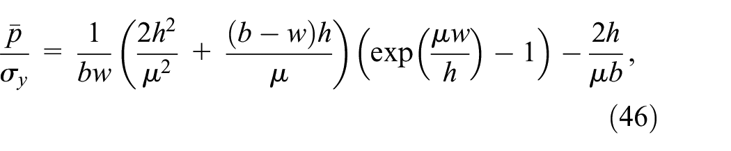
Based on a slab analysis of the sample shown in Figure 6 with the Cartesian coordinate’s origin in the sample’s mid-plane and the $x$ axis parallel to $b$ , it can be shown ¹¹⁸ that for small values of $\mu b/h$ :

$$P_{\mathrm{ave}}=\frac{F_{\mathrm{p}}}{\mathrm{bw}}=\frac{2{\overline{\sigma }}_{\mathrm{ave}}}{\sqrt{3}}(1+\frac{\mu b}{2h})=\frac{2{\overline{\sigma }}_{\mathrm{ave}}}{\sqrt{3}}(1+\frac{\mathrm{mb}}{4h})$$

(39)

where h is the instantaneous height of specimen, b and w are instantaneous width and depth, respectively, ${\overline{\sigma }}_{\mathrm{ave}}$ is the effective stress, $P_{\mathrm{ave}}$ , $F_P$ , $m$ , and $\mu$ are average pressure, plane strain load, sticking friction factor, and Coulomb’s friction coefficient, respectively. The analysis assumes a uniform state of effective stress in the sample.

The slab method-based analytical solution of PST assumes a constant friction coefficient $\mu$ and a homogeneous plastic deformation through the cross-section of the sample. The general solution for converting the force-displacement into an equivalent stress-strain curve can be written as:

$${\overline{\sigma }}_{\mathrm{ave}}={\sigma }_y/f$$

(40)

$$\overline{\epsilon }=-f{\epsilon }_3$$

(41)

where ${\epsilon }_3=\ln (h/h_0)$ and $f$ is a correcting factor. It should be noted that the formula for the equivalent strain depends essentially on the adopted yield criterion; for example, while the Tresca criterion directly leads to equation (41), the von Mises leads to:

$$\overline{\epsilon }=\frac{2}{\sqrt{3}}{({\epsilon }_2^2+{\epsilon }_2{\epsilon }_3+{\epsilon }_3^2)}^{0.5},$$

(42)

where ${\epsilon }_2=\ln (b/b_0)$ ; however, because of two reasons: (1) ${\epsilon }_2$ and ${\epsilon }_3$ are not independent, and (2) ${\epsilon }_2<<{\epsilon }_3$ , the equivalent strain can be written in the general form of equation (41).

Petersen et al. ¹¹⁹ proposed:

$$f=(\frac{2}{\sqrt{3}}(b-w)+w)/b\approx 1.155-0.155\frac{w}{b}$$

(43)

where $b$ is the instantaneous breadth. A common relationship for obtaining $b$ is that proposed by Mirza and Sellars ¹²⁰ :

$$b=b_0(1+C-C{(h/h_0)}^n),$$

(44)

where the exponent $n\approx 0.2$ for aluminum samples lubricated with graphite, ¹¹⁹ and $C$ is the spread coefficient for the sample dimensions before and after a test:

$$C=\frac{(b_f/b_0)-1}{1-{(h_f/h_0)}^{0.5}}.$$

(45)

Note that the exponent 0.5 is a fitting parameter. ¹²⁰

The flow stress in PST is conventionally denoted as ${\sigma }_y=2k$ , with $k$ being the flow stress in pure shear (torsion); however, the relationship changes as the friction condition varies between sliding and sticking. Silk and van der Winden ¹¹⁷ defined a parameter $z_0=\left(\frac{h}{2\mu }\right)\ln \left(\frac{1}{2\mu }\right)$ to identify the friction conditions. For the sliding friction ( $2z_0>w$ ), the flow stress is connected to the average pressure ( $\overline{p}=\frac{F}{\mathrm{wb}}$ ) via:

$$\frac{\overline{p}}{{\sigma }_y}=\frac{1}{\mathrm{bw}}(\frac{2h^2}{{\mu }^2}+\frac{(b-w)h}{\mu })(\exp \left(\frac{\mu w}{h}\right)-1)-\frac{2h}{\mu b},$$

(46)

and for the sticking friction ( $2z_0<0$ ) via:

$$\frac{\overline{p}}{{\sigma }_y}=1+\frac{w}{4h}-\frac{w^2}{12\mathrm{hb}}.$$

(47)

Furthermore, the function for the partial sticking friction condition ( $w>2z_0>0$ ) can be developed ¹¹⁷ as well, which is not presented here.

Recently, Chermette et al. ¹²¹ proposed a different approach to develop a new analytical method to solve the above-mentioned general formulas of equivalent strain and stress. In this work, they proposed to use data of a uniaxial tensile test to obtain the correction factor. They applied the Tresca yield criterion and proposed the flow stress as:

$$\frac{\overline{p}}{{\sigma }_y}=\frac{h}{\mu w}(\exp \left(\frac{\mu w}{h}\right)-1)+\frac{h}{4w}.$$

(48)

The correction factor is defined as:

$$f={\sigma }_{\mathrm{y},\mathrm{ref}}/{\sigma }_{\mathrm{UTT}},$$

(49)

where ${\sigma }_{\mathrm{UTT}}$ is the stress obtained from the uniaxial tensile test, and ${\sigma }_{\mathrm{y},\mathrm{ref}}$ is reference stress that should be found from ${\sigma }_{\mathrm{UTT}}\times {\epsilon }_{\mathrm{UTT}}={\sigma }_{\mathrm{y},\mathrm{ref}}\times {\epsilon }_{\mathrm{y},\mathrm{ref}}$ . The work of Chermette et al. ¹²¹ has been validated only for the sliding friction condition. Moreover, their model is developed for tools with finite radii, while here we adopted a version for a tool without a radius.

Split-Hopkinson pressure bar test

The test is generally involved generating a wave to ideally produce a one-dimensional stress wave in its sample. A common technique for the indirect measurement of the flow stress by SHPB test is strain measurement in its sample. In this technique, one measures length changes in the sample by comparing the velocities of the sample at both ends ( $V_{\mathrm{I}}$ and $V_{\mathrm{T}}$ in Figure 7); this is in contrast with indirect measurement of the effective stress by other tests reviewed in this work. In this technique, different strains induced in the incident and transmission bars are measured using strain gauges (e.g. ${\epsilon }_{\mathrm{I}}$ , ${\epsilon }_{\mathrm{T}}$ , and ${\epsilon }_{\mathrm{R}}$ being the incident, transmission, and reflection strains in Figure 7, respectively). Adding these strains algebraically together, one can find the effective strain in the sample assuming a one-directional stress wave development and propagation. This enables the measurement of deformation in the specimen by integrating the strain with respect to time along the one-dimensional deformation path. Stresses in the sample are recovered using a set of applicable elastic or plastic deformation criteria, a suitable constitutive law, and elastic or plastic energy principles. Such a measurement ignores shear and transverse wave propagation in the sample.

Given the high dynamics nature of the measurement, both experimental and analytical considerations should be planned very carefully. While a wide range of analytical considerations is utilized for the test due to the diversity of the test modes and material types, there are some common experimental requirements for all these tests: for example, very high-resolution data acquisition, minimized friction at the contact points, precise alignments with electronic modules, and sophisticated control systems.

Because the test is mostly used for the room temperature behavior of material and rarely used for hot flow characterization or its associated phenomena, the test’s post-processing techniques are not reviewed in detail here. The interested readers can find further details in the literature, for example, in Chen and Song, ⁴⁴ Bagher Shemirani et al., ⁴⁸ Gray et al., ⁵⁶ and Dai et al. ¹²²

Standards

Compression and torsion tests are generally performed using different settings and specimens, while a few standards are available on tensile testing, (see for example references^123–127).

ASTM E209-18¹²⁸ does not provide enough details for the experimental determination of hot flow curves in compression tests. Existing standards do not provide sufficient details for the experimental practice of determining the flow curves in compression tests. In ASTM E 209-18, ¹²⁸ a constant crosshead speed is also allowed for; however, this results in a large variation of strain rate if high strains are attained.

There is a real need for significant developments and improvements to provide adequate standards for mechanical tests.

Advanced analyses

Advanced analyses comprise direct methods (closed-form solutions) and inverse methods (either numerical or analytical). Also, continuous or interrupted (multi-pass) modes of deformations are useful to classify the existing advanced analyses.

Direct methods (closed-form solutions)

Direct methods are those that take the raw load-deformation data as input directly into a closed-form solution to identify the material flow behavior. The solution allows tracing the development of the effective stress and strain, for a given strain rate and temperature, at a test sample’s material point. Direct methods have been extensively used with all of the four main tests. This section reviews some advanced direct methods available for the mechanical tests.

Inverse methods

The main objective of performing a mechanical test is to determine the material parameters. In several studies, including those of interrupted deformations, the advanced closed-form solutions of the tests are not adequate to correlate the test data and their flow behaviors. This is the case with a study that requires the constitutive parameters as its input, for example, during numerical analysis or during interrupted tests.

The parameter estimation method, ¹²⁹ which is a sub-class of “inverse methods,” employs a combination of a direct method and minimization of errors to determine the unknown parameters. The theory required for numerical analysis of the tests or their closed-form solutions together with experimental raw data is the ingredients for an inverse method. An inverse method also involves the construction of a cost function and its minimization to identify the optimum parameters. Minimization of a cost function (objective function) is a major component of the parameter estimation method. In general, the cost function may have several minima and it is necessary to ensure that the optimization process reaches the global minimum of the cost function. This condition is more likely to be met when the initial guess provided for the design variables is close enough to the global minimum. If a good initial guess is provided, then the local minimum obtained by solving the optimization problem and the global minimum will coincide. Providing a good initial guess for the optimization involves the utilization of a simple closed-form solution.

Search methods are the most important element of an optimization technique. Two types of zero-order search methods, namely Powell’s ¹³⁰ Method and the simplex method of Nelder and Mead, ¹³¹ have been used widely to perform the optimization required for the parameter estimation technique. The reason is that the higher-order search methods need the evaluation of the derivatives of the cost function at many points. These derivatives have to be calculated numerically, which can considerably increase the computational time. Moreover, due to the existence of experimental noise in the cost function, these derivatives (usually used for determining the search vector) are not reliable; however, higher order methods (e.g. those using the Hessian matrix ¹³² ) have been used by some researchers ¹⁹ to post-process the test results. To avoid derivative-related difficulties, one can utilize global optimization methods, which are zero-order search methods, such as particle swarm optimization, genetic algorithms, etc., in the inverse method.

Continuous and interrupted tests

Continuous tests are typically worked to simulate some key forming processes, such as forging and extrusion, in which the material is deformed in a single operation. Alternatively, when a material is deformed in a multi-step fashion, such as multi-stage rolling and radial forging, static recrystallization, and recovery play a key role in its constitutive behavior. Multi-step deformation simulations are the analytical components for thermo-mechanical processing.^23,133,134 Interrupted tests have been widely used in the literature to physically simulate such industrial scenarios.^135,136

The advantages of stepwise deformation can be summarized as follows:

1. The load to deform material at high strains is much lower than that for uninterrupted deformation so that the elastic deformation of the deformation tool is smaller;

2. During the interruption, the deformation heat can be conducted off so that the isothermal flow curve is approximated.

Continuous torsion test

Since the specimen geometry does not ideally vary during the torsion test, a constant strain rate is easily obtained at a given radius by keeping the number of revolutions per minute constant. The majority of the physical simulations are based on a continuous deformation starting with a normalized and uniform microstructure in the sample. The deformation is carried out once under a constant strain rate to provide a given amount of plastic effective strain in the sample. Such single-hit tests are mainly useful to study a one-hit deformation scenario and several practical issues for process optimization or to establish and calibrate basic deformation phenomena for example dynamic softening and recrystallization.

Effective length

Some of the researchers of the hot torsion test take into account the contribution of the angular rotation of the filet between the uniform section and the shoulder. Pöhlandt ¹³⁷ proposed $L_{\mathrm{eff}}$ as the effective length. $L_{\mathrm{eff}}$ is obtained by a semi-empirical method, introducing the concept of the active length of the specimen as:

$$L_{\mathrm{eff}}=L5+2{\hat{L}}_{\mathrm{eff}}$$

(50)

where ${\hat{L}}_{\mathrm{eff}}$ has been defined as (see Figure 17)

$${\hat{L}}_{\mathrm{eff}}={\int }_0^{R5}{\left(\frac{R4}{R\left(z\right)}\right)}^{\left(\frac{3+m+n}{m+n}\right)}\mathrm{dz}$$

(51)

or

$${\hat{L}}_{\mathrm{eff}}={\int }_0^{\frac{\pi }{2}}{\left(\frac{R4R5\cos \left(\xi \right)}{R4+R5(1-\cos \left(\xi \right))}\right)}^{\left(\frac{3+m+n}{m+n}\right)}d\xi$$

(52)

Figure 17.

Illustration for Pöhlandt’s formula.

Equation (52) ⁶³ implies that the active length depends on the material properties as well as geometry. It has to be mentioned that equation (55) is only applicable if the constitutive equation is similar to that given by $\tau =G{\gamma }^n{\stackrel{·}{\gamma }}^m$ .

Interrupted torsion test

Interrupted or multi-hit physical simulations are far more complex than the continuous (single-hit) ones to perform and to interpret their results. A dedicated theory has been developed by Khoddam and Hodgson ¹¹ to account for the heterogeneous static recrystallization in the torsion test. Due to experimental limitations of measuring deformation parameters and their distribution in the sample during deformation and during the interruption period, numerical results of heterogeneous static recrystallization in the torsion test sample can be used to verify such theories. The presented theory ¹¹ takes advantage of an inverse solution and a cost function to estimate static recrystallization but relies on the closed-form solution of the test.

Data classification

The theoretical framework and its solution presented in Khoddam and Hodgson, ¹¹ Khoddam and Hodgson ¹³ require the construction of several torque-twist data types which are defined and employed in the work. The detailed terminologies (e.g. $M,\tilde{M},\mathbb{M}\mathrm{and}\tilde{\mathbb{M}}\mathrm{vs}.\theta \mathrm{and}\mathrm{\Theta }$ ), the procedures to construct the data and their numerical interpolations which are needed for the inverse solution can be found in Khoddam and Hodgson. ¹³

Procedure for the inverse interrupted solution

The procedures to carry out the inverse calibration/solution of a kinematic model based on the torsion test’s data have been presented in Khoddam et al. ¹² This allows estimation of the fractional softening and its distribution in the sample in a multi-layered fashion. The calibration was carried out by generating the experimental torsion data in an equally spaced grid within the entire deformation range with respect to the interruption time and the pre-strain. The inverse method utilized in Khoddam et al. ¹² offers a non-FE inverse calibration of SRX kinematics. It involved iterative solutions of the test in an optimization framework. Steps and procedures for this method have been demonstrated as a flow chart in Figure 18 for a power-law constitutive equation.

Figure 18.

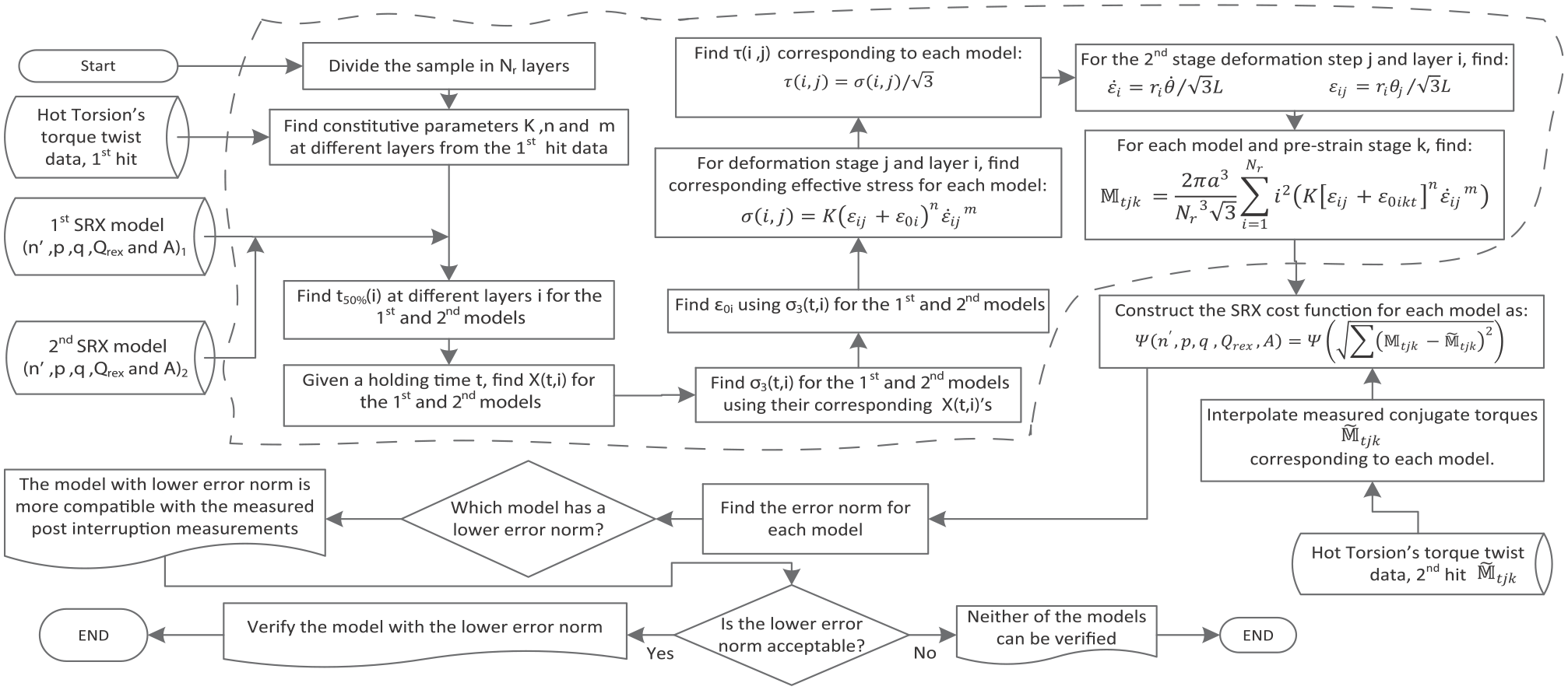
A flow chart to evaluate and compare two proposed SRX kinetic models together and to measure their accuracy. It also shows the borders between the verification tool, to assess a proposed SRX model, with the multi-layer formulation ¹³ which is enclosed inside the dashed border.

The solution compares the experimental multi-hit torque-twist data to its corresponding simulated one and identifies its best kinematic model parameters by minimizing the difference between the two data sets. ¹² The closed-form multi-layer formulation in Figure 18 serves as an iterative solver of the torsion test which provides the analytical components needed in the optimization-based assessment framework.

Sample results on a typical distribution of fractional softening in the test sample

Based on the theoretical framework presented in Khoddam and Hodgson, ¹¹ , Khoddam and Hodgson ¹³ sample solutions were carried out in Khoddam and Hodgson ¹¹ to demonstrate the extent of heterogeneities for the fractional softening $X$ in the sample and its impact on the identified kinematic model parameters (see Figure 19).

Figure 19.

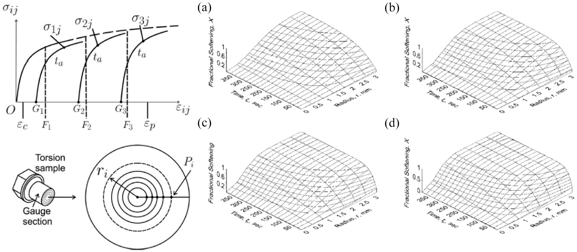
Left: Illustrating a relaxed flow stream set corresponding to a holding time of $t_a$ ¹¹ and, Right: Distribution of fractional softening, ¹¹ $X$ , in the radial direction along a straight radius after twisting the sample by: (a) ${\theta }_F=2.07$  rad, the maximum pre-strain of ${\epsilon }_F=0.2$ , (b) ${\theta }_F=3.10$  rad, the maximum pre-strain of ${\epsilon }_F=0.3$ , (c) ${\theta }_F=4.14$  rad, the maximum pre-strain of ${\epsilon }_F=0.4$ , and (d) ${\theta }_F=5.17$  rad, the maximum pre-strain of ${\epsilon }_F=0.5$ . For all four cases, the sample deforms at an angular velocity of $\stackrel{·}{\theta }=0.103$  rad/s.

The sample solutions obtained in Khoddam and Hodgson ¹¹ were compared to the results obtained based on a kinematic model according to the conventional torsion test data reduction methods. A sample comparison has been shown in Figure 20.

Figure 20.

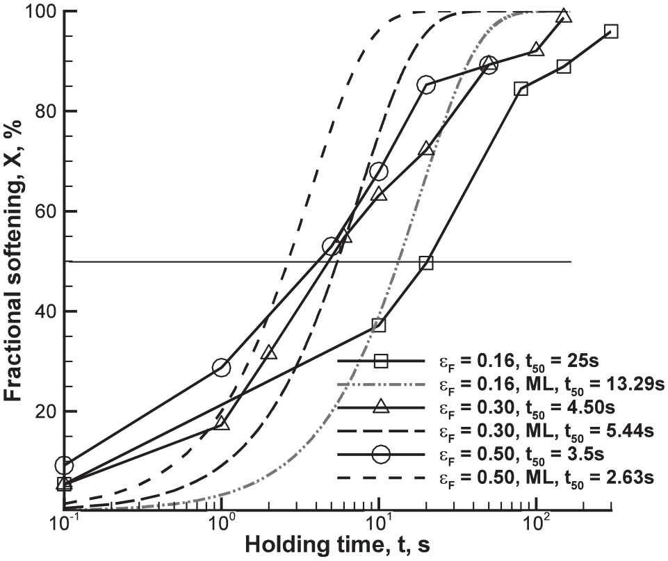
Comparison of softening fraction S-shaped curves and $t_{50\%}$ using traditional and multi-layered (ML) inverse solutions. ¹²

The mathematical framework was implemented for a double-hit torsion test results with an austenitic Ni30-Fe alloy sample which was tested at $1000°\mathrm{C}$ and a strain rate of $1s^{-1}$ . This enabled the study of the extent of deformation heterogeneity in the sample and evaluation of the accuracy of the measurements and characterizations based on the conventional post-processing of the test data. Also, the identified kinetics of static recrystallization was compared with that based on the conventional methods. It was found that based on the interruption scenario, the critical radius, where the fractional softening saturates in the sample, could grow to 90% of the gauge radius. This was found to be the case for a holding time of 5 s or less. Also, it was found that in an innermost cylindrical core of the specimen, comprising 20% of the gauge radius, the critical time was larger than 250 s. It was concluded that the heterogeneous recrystallization in the specimen resulted in the indirect measurement of the effective stress during the second pass and, subsequently, resulted in errors in the second-tier indirect measurement, that is, the SRX kinematic parameters. The errors were found to be critical with short holding times ( $\le 10s$ ) and/or low pre-strains of ${\epsilon }_F\le 0.3$ .

Continuous compression test

The velocity field proposed by Avitzur ⁷³ and that proposed later by Khoddam ³⁵ account for the barrelling; however, the former does not allow for a proper friction factor identification. Moreover, neither of these fields can properly accommodate foldovers in the test sample.

Given the heterogeneous deformation in the sample, it can be shown that material’s forming limit is significantly underestimated by commonly used post-processing methods; the maximum strain in the test samples is generally higher than that anticipated in the gauge section (or inside the equivalent non-barrelled sample) based on an ideal/uniform deformation. The latter model, ³⁵ the exponential profile model (EPM) was proposed to post-process the ACT data.

Comparing velocity components of CPM and EPM

The motion of a material point in the sample can be studied purely based on the model represented by a cylindrical profile model (CPM) or the proposed EPM ³⁵ without linking it to the cause of the motion (e.g. the applied force or developed friction). This kinematic study was conducted in a case study fashion to compare the typical velocity fields for a CPM and the EPM. The assumed geometrical values for the case study included: $B=0.04$ , $\stackrel{·}{H}=10$ , $H=8$ , $D_0=10$ , and $H_0=16.$ Figure 21 compares different aspects of the velocity components used in the cylindrical and exponential profile models.

Figure 21.

Comparison of normalized velocity vector fields and their components for CPM and EPM. (a and b) Velocity components for CPM, (c and d) velocity components for EPM, (e) ${\overrightarrow{\phi }}_{\mathrm{EPM}}$ , and (f) difference between ${\overrightarrow{\phi }}_{\mathrm{EPM}}$ and ${\overrightarrow{\phi }}_{\mathrm{CPM}}$ (see equation (25)).

Contrary to the CPM, the EPM velocity field accounts for the barrelling; however, neither of the models can capture the complex variations of velocities post-foldover.

Foldover

To model the foldover, the deforming sample must be divided into different zones with the velocity components being functions of both $r$ and $z$ . For example, Avitzur and Kohser^138,139 proposed a composite velocity field to account for foldover. They divided the deforming sample into two different zones with continuous velocity components normal to the zones’ interface. Available solutions of the ACT cannot adequately account for the onset of foldover which has a critical value to properly post-process the test data after the foldover’s onset.

EPM’s flow identification: A multi-layer approach

Recently, a combined multi-layer and EPM approach was proposed by Khoddam and Hodgson ¹⁴⁰ to identify the material’s flow curve. They accounted for the non-cylindrical sample in their formulation and derived a closed-form solution for the flow stress by discretizing the barrelled sample into a finite number of cylindrical slices of different radii and found the effective stress in terms of the number of layers, the individual layers’ radii, friction factor, and the current height of the sample. It was shown that their solution approaches that of Avitzur ⁷³ for the special case of no-barrelling.

Experimental limitations for employing advanced methods

To implement the advanced solutions of ACT, including EPM, one needs to measure the mid-plane diameter of the sample as the function of the sample’s height changes. Currently, available compression test rigs are incapable of such measurement. Therefore, virtual finite element generated test data are used in studies of such solutions. ³⁶

The next section provides a conceptual experimental setup to measure the required barrelling data for the EPM method, namely $H-D-B$ . This will allow the implementation of advanced techniques based on real test data.

Concurrent measurement of the EPM’s barrelling data

Rasmussen et al. ¹⁴¹ used the Rastegaev ⁸¹ sample in an upsetting device with a transducer ring. While they used the transducer in conjunction with the Rastegaev sample, one notes that the ring is primarily suitable to measure the sample’s mid-plane diameter $D$ . A conceptual design of the setup is shown in Figure 22 as the perspective, exploded and section views.

Figure 22.

The conceptual design of a barrelling measurement transducer setup: (1) sample, (2 and 3) platens, (4 and 5) lower and upper compression-guiding plates, respectively, (6) middle transducer ring, (7) inductive diameter transducers and their contact tips, (8 and 9) lower-upper compressive springs to keep the transducers’ tips at the sample’s mid-plane during the entire test, and (10) connecting rods. Measuring $D$ when the material properties are axisymmetric, it is sufficient to measure the diameter in only one direction.

We propose to employ the conceptual design in Figure 22 to concurrently measure the barrelling data needed for the advanced EPM analysis; the design enables the measurement of $H-D-B$ . Given the initial geometry ( $D_0$ and $H_0$ ), the mid-plane and top-plane diameters, $D$ and $d$ , respectively can be correlated as ⁷⁷ :

$$d=\frac{\sqrt{5H(9D_0^2{H}_0-4D^{2}H)}-2\mathrm{DH}}{3H}$$

(53)

Also, an equivalent radius $\overline{R}$ to be used for the estimation of EPM’s barrelling parameter, $B$ , can be found as:

$$\overline{R}=0.5D_0\sqrt{\frac{H_0}{H}}$$

(54)

Details on calculations of the EPM’s barrelling parameter $B$ based on $\overline{R}$ , $H$ , $D_0$ , and $H_0$ can be found in Khoddam et al. ¹⁴²

Interrupted compression test

Yanagida et al. used an inverse analysis of the compression test and a coupled thermo-mechanical finite element analysis to calculate the constitutive parameters under dynamic recrystallization. ¹⁴³ They also utilized an inverse analysis to obtain the constitutive equation which takes into account the inhomogeneous strain and temperature distributions. They applied the identified parameters to evaluate the softening fraction in a double compression test. ¹⁴ More recently, Meng et al. ¹⁶ carried out some experiments, inverse analyses, micrographic investigation, finite element method (FEM), and regression analyses to obtain the material genome ¹⁶ for a Fe–0.15C–0.2Si–1.4Mn–0.03Nb alloy, these were used to describe the static and dynamic kinetics of microstructural evolution for the alloy.

While such studies are useful to understand the extent of the fractional softening in the sample, to convert the multi-hit ACT data to flow curve and to identify its corresponding kinematic model, a non-finite element inverse analysis is preferred; to account for the heterogeneous fractional softening in the sample after the interruption is quite complex and the conventional flow identification methods are unqualified for the task.

Sample applications: thermo-mechanical processing and physical simulation for steel

Although there exist a wide variety of metal forming operations, the basic aim is to produce the desired shape change. However, a class of processing, known as thermo-mechanical processing (TMP), is extensively used in metal forming to improve the product properties by engineering its microstructure during the process.

While early work used full-scale plant trials to develop the basic concepts, the development of advanced physical simulation techniques enabled more laboratory-based developments. This significantly reduced the cost and also provided greater insight into the physical processes taking place (e.g. dynamic and static recrystallization) for a given composition and process. As shown in the following, there are only a limited number of cases where the laboratory simulation can exactly match the process conditions and it is more usual to have to extrapolate the laboratory results using models or other techniques.

Thermo-mechanical processing of steel

TMP is widely practised throughout the world to produce steels with improved mechanical properties without the need for subsequent heat treatment. It also generally lowers the use of alloy element additions, which improves weldability and reduces costs and produces final properties not achievable by any other technique.

The various techniques can be divided into those that involve control of the deformation processes or control of the post deformation cooling history. While the technological aspects of TMP are well understood, there are still several theoretical issues that need to be resolved, particularly if generalized models are to be constructed. At the same time, there are now TMP processes developed based on either microstructure manipulation, such as the formation of ultrafine ferrite through strain-induced transformation, or through new plant configurations. The latter involves the close coupling of the casting and working processes and involves a much more integrated approach to TMP, while also requiring the development of new microstructure evolution models.

A large portion of the microstructure mechanisms considered by the physical metallurgist plays a role in the TMP of steel, namely recrystallization, grain growth, transformation, and precipitation. These combine, often through complex interactions, to dictate the sequence of microstructural events that lead to the end microstructure, which plays a large role in determining the mechanical, physical, and chemical behavior of the final product.

The commercial exploitation of TMP began over five decades ago with the introduction of controlled rolling, particularly in the manufacture of plate products. In these early instances, the rate of recrystallization in the austenite was reduced so that strain could be accumulated in the microstructure during finish rolling. Accumulated strain leads to fine ferrite grain sizes following transformation.

In the intervening period to the present, a range of commercial TMP processes has been developed (and exploited commercially) for a wide range of hot deformation operations. A cross-section of these is summarized in Table 2, along with the important microstructure and thermal-mechanical aspects.

Table 2.

Selected thermo-mechanical processes and their microstructural, mechanical, and thermal challenges.

Process	Description	Microstructure processto be controlled	Thermal and mechanical challenges
Conventional controlled rolling/forging	Finishing hot forming below the recrystallization stop temperature (RST) to improve strength and toughness	Static RecrystallizationStrain induced precipitation	Temperature control Higher rolling loads
Accelerated cooling	Water or air cooling through the transformation at moderate rates	Transformation	Heat transfer Temperature uniformity Residual stresses
Direct quenching	Water or other high-speed quenchants to form more hardenable microstructure	Transformation	Heat transfer Temperature uniformity Residual stresses
Quench and selftempering	Rapid quenching of a stock surface using water to form martensite surface layer which is then auto tempered by heat conducted from the center of the bar	Transformation	Heat transfer
Rod colling	Forced air or retarded cooling of rod/bar to remove heat treatment before cold forming	Transformation Annealing	Heat transfer
Warm forming	Deformation of a predominantly ferrite microstructure	Recrystallization texture	Rolling mechanics Heat transfer
Intercritical rolling	Deformation of mixed austenite and ferrite microstructure for improved strength and toughness	Transformation Recrystallization Precipitation Texture	Rolling mechanics to predictrolling load

There are also a large number of thermal and mechanical aspects that also need further work, and some of these will also be raised (Table 2 also highlights some particular areas). Table 2 reveals that TMP is carried out in two areas of manufacture: (i) during deformation at elevated temperature, and (ii) during cooling to room temperature following deformation. This natural division will be used as the framework in discussing the microstructural and mechanical issues confronting current TMP approaches.

Steel deformation

Steel forming, in the context of TMP, can be mainly classified as hot and warm working.

Hot-working

The basic concepts of TMP were initially developed for use in the control of deformation in plate mills where there was a need for new products with improved strength, toughness, and weldability. The last of these results from a lower alloy element addition, whereas the former two are achieved through grain refinement.

The ferrite grain size is refined by increasing the density of ferrite nucleation sites before the start of the transformation. The nucleation site density, in turn, is raised in one of two ways. The first, and most widely applied, involves increasing the grain boundary surface area/unit volume (and intergranular sites) by retarding recrystallization. This approach is termed conventional controlled rolling. The second employs repeated recrystallization between subsequent deformation passes and is termed Recrystallization Controlled Rolling (RCR). This approach relies on the presence of a fine dispersion of TiN precipitates which are formed during solidification and reheating. However, the removal of N (in TiN precipitates) decreases the strength of the steel, which counteracts the strengthening achieved by grain refinement.

Hence true RCR is generally combined with extensive precipitation hardening through the addition of moderately high levels of V (also with higher N contents). The more common scenario is to use RCR concepts during the roughing phase of a CCR process. The fine TiN particles then provide further improvements by markedly reducing the size of the heat-affected zone during welding. The key outstanding research issues in these processes lie with the development of adequate generalized mathematical models to predict the microstructure during processing. Although there is a range of mathematical models to predict, for instance, the transformed ferrite grain size as a function of deformation parameters, ¹⁴⁴ none are sufficiently generalized to permit the prediction of grain size outside a limited range of compositions and conditions.

Warm working

Over the last three decades or so, several producers of steel strip have found that considerable benefit can be gained by running their hot strip mills at temperatures 70°C or more below normal finishing temperatures (see Harlet et al., ¹⁴⁵ Parks et al. ¹⁴⁶ ). This practice, known variously as warm or ferritic rolling, has the potential to broaden the product range and lower the production cost of the hot-rolled strip.

Changing the rolling temperature from the “hot” to the “warm” regime leads to a considerable change in the physical metallurgy. This is a consequence of the fact that the austenite to ferrite phase transformation occurs before, or during, deformation. In the case of the former, issues arise with respect to the microstructure evolution of ferrite at elevated temperatures. In the case of the latter, which involves deformation in the two-phase region, these are combined with the mutual influence of each phase on the microstructure and, probably, more importantly, the substructure of the other.

Transformation is an alternative to deformation to control the manufacturing of steel. It is beyond the scope of physical simulation via mechanical tests. Such processes are usually simulated using other physical simulation rigs such as deformation dilatometers. The interested reader can refer to Nishioka and Ichikawa ¹⁴⁷ for details of such controls.

Physical simulation approaches

The development of the above TMP approaches was initially through full-scale mill trials. However, the development of the hot compression and hot torsion tests at about the same time led to large scale laboratory investigations. In particular, the concept of controlled rolling involved determining the temperature and alloying conditions under which recrystallization was retarded to be longer than the inter-pass period. The strains, strain rates, and temperatures of plate rolling (Table 1) were similar to those that could be achieved in the ACT and hence the study of the effect of composition using these tests led to the development of the Nb microalloyed steels. The role of other microalloying elements, such as V and Ti was also studied in this physical simulation.

The ACT is limited by the total amount of strain that can be applied and so could not take account of the microstructure refinement during the roughing part of the test. The so-called Tnr test using hot torsion was developed by Jonas et al. at McGill university to address this issue. Here the sample is reheated and cooled at a constant cooling rate with deformation applied at regular intervals. The change in work hardening behavior, determined from the average stress for each deformation provides insight into the level of recrystallization, while it is also possible with this test to determine the critical transformation temperatures for the start and finish of ferrite formation during warm rolling.

The further reproduction of actual rolling schedules on hot deformation equipment has been also obtained in-plane strain compression, where it has been extended to hot strip mills, although it is generally not possible to obtain the exact temperature profile during the latter stages of rolling where conduction to the work rolls is important. Hodgson et al. further extended the torsion physical simulation to include the strains and inter-pass times in rod and bar mills, but it is not possible to simulate the actual strain rates and temperature changes. However, the work did highlight the likely role of strain accumulation leading to dynamic and metadynamic recrystallization.

In summary, the laboratory simulation can lead to general insights into the likely microstructure evolution processes in commercial rolling, but outside of plate rolling it is generally necessary to make simplifications to the strain rate and thermal history of the sample.

Conclusions and the future works

Flow curve identification and the flow curve-based studies start at a physical simulator level and therefore the physical simulation platform and its associated analytical post-processor (solver) need to be chosen carefully to fulfill several criteria before they can be adopted at a scientific or engineering level.

For engineering and industrial applications, the questions to be answered by a physical simulation are typically far more basic and simpler compared to those posed by scientists. The currently used existing physical simulators and studies have provided valuable insight and helped them to optimize their processes and to reduce the costs.

From a scientific perspective, the requirements are much higher and therefore one has to choose the platform and its associated analytical method very carefully; as such physical simulations are often used to validate complex hypotheses, indirectly measure second-tier deformation parameters and monitor the progress of several dynamic phenomena with time. The barriers to reduce the test’s load-deformation data into flow curve include inevitable deviation of the tests from their ideal deformation scenarios and our limited understanding of the multi-disciplinary interactions between the materials and properties. Significant gaps and deficits exist, analytically and experimentally, to indirectly measure the effective stress-strain reliably based on the available mechanical tests reviewed in this article. Therefore, serious questions are posed on the reliability and repeatability of the existing measurements and their industrial applications due to the deficient fulfilment of the criteria. Table 3 presents a concise summary of the reviewed tests, their merits and disadvantages.

Table 3.

A simple comparison of the reviewed mechanical tests.

	Tension	Torsion	Compression	SHPB
Stability of deformation Simple geometry for analysis	Robust for elastic deformation and that before necking, only gauge section deforms	Stable geometry for large plastic strains, 148 only gauge section deforms	Good before foldover and barreling, 149 entire sample deforms	Similar to compression case, more challenging to measure, entire sample deforms
Applicability on simulating deformation states, e.g. load reversal	Limited to uniaxial forming, some attempts to interpret test results after necking by combined numerical-analytical-experimental methods, prone to buckling under compression (reversal)	Dominantly, shear deformation; unable to resemble most forming scenarios, lower flow curves than other tests, 93 easy load reversal	Uniaxial compression can extend to multiaxial using new barreling models, unable to reverse the loading	Similar to the compression case, only a few published works are available, unable to reverse the loading
Application forlarge stresses and strains	Plastic stresses and strains can only be interpreted using inverse methods	Commonly used for highest achievable strains and stresses	1. Limited by stroke and large heterogeneity 2. Strains larger than those of tensile and smaller than those of torsional tests	Mostly used for cold-warm deformations and super plasticity
Key limitations	1. Hard to keep the strain rate constant 2. Unsuitable for plastic deformation at elevated temperatures	Strain rate changes radially and linearly	1. Barreling dynamically changes the geometry 2. Friction brings uncertainty 3. Foldover is hard to model/ measure	Extremely fast deformation; data acquisition is limited by the available technology

This article reviewed the most commonly used mechanical tests to indirectly measure materials’ hot flow behavior and the second-tier material properties which rely on the flow curves. The unique combination of the pros and cons for each test was reviewed in detail to choose the optimum test which suits a given application. It was highlighted that only a small number of models exist to identify flow and softening properties with limited transferability/consistency depending on the tests used to derive them. The gap and deviations from the ideal case become much wider when measuring other properties which rely on indirect measurement of the flow curves. The complications are found to increase when the flow stresses with at least one unloading or relaxation are involved.

It might be concluded that the available physical simulators and their solvers deviate inevitably and significantly from the ideal uniaxial deformation under constant strain rate and temperature. To minimize the impact of the deviations, a significant number of developments on both experimental and analytical methods are needed. These are essential to obtain reliable flow curves which are independent of the chosen physical simulator.

Recently developed advanced analyses reduce some of the limitations such as accounting for multiple regimes of hardening, deformation outside the gauge section, barrelling/multi-axial deformation, friction, and non-homogeneous hardening/softening of the sample during multi-step deformation scenarios. However, more advanced theories are needed to further reduce the limitations. Also, new data types have to be measured concurrent to the load-deformation data to enable the implementation of the advanced analyses.

Some future experimental developments in mechanical testing include:

• Concurrent measurement of length and temperature changes during high twist torsion.

• Provision of adequate standards for the mechanical tests.

• Development of new axisymmetric and plane strain compression test rigs to:

Some future analytical developments in mechanical testing include:

• Models to account for barrelling, foldover, friction variation, flow curve identification at a representative point.

• Dedicated post-processing theories for the interrupted tests.

• High strain rate simulation with advanced theoretical solvers.

• With regards to the future of the parameter estimation technique applied to the mechanical tests, several interesting prospects for future research are available.

• Development of numerical methods for calculation of initial and post deformation temperature distribution.

• To employ each non-ideal mechanical test as avenue to study multi-axial loading/deformation scenarios to present a more realistic simulation of the multiaxial stresses in material under real forming process.

• Contributions in the new fields of the inverse method to use the numerical-experimental analysis of the mechanical tests to explore and explain metallurgical phenomena during the deformation.

• Inclusion of length changes in end-free torsion test to explain the evolution of texture during the test.

• Comparison between the softening due to heat generation during the test and the hardening due to work hardening in a manner that is independent of the type of constitutive equation chosen.

• Use of inverse solution of the mechanical tests to determine the coefficients which describe thermal boundary conditions during the hot tests.

Experimentally, thermo-mechanical processing is a mature concept in the steel processing industry and there has been little change in the processes involved over the past few decades. Assuming a flow model as the measured data, most of the research is focused on the second tier and indirect measurement of the thermo-mechanical process parameters and to the refinement of our understanding or in the representation of the process in mathematical models. This is where the physical simulations and their resulted measurement can play the most significant role. At the same time, new processes are being developed which are attempting to develop ultrafine ferrite grains through a strain-induced transformation during hot rolling. Other changes are in the range of future potential configurations that may be possible with the new near net-shaped casting and direct rolling processes. Both of these developments indicate new areas of theoretical research that are required.