Analysis of Timoshenko beam with Koch snowflake cross-section and variable properties in different boundary conditions using finite element method

Abstract

This study analyzed a Timoshenko beam with Koch snowflake cross-section in different boundary conditions and for variable properties. The equation of motion was solved by the finite element method and verified by Solidworks simulation in a way that the maximum error was about 2.9% for natural frequencies. Displacement and natural frequency for each case presented and compared to other cases. Significant research achievements illustrate that if we change the Koch snowflake cross-section of the beam from the first iteration to the second, the area and moment of inertia will increase, and we have a 5.2% rise in the first natural frequency. Similarly, by changing the cross-section from the second iteration to the third, a 10.2% growth is observed. Also, the hollow cross-section is considered, which can enlarge the natural frequency by about 26.37% compared to a solid one. Moreover, all the clamped-clamped, hinged-hinged, clamped-free, and free-free boundary conditions have the highest natural frequency for the Timoshenko beam with the third iteration of the Koch snowflake cross-section in solid mode. Finally, examining important physical parameters demonstrates that variable density from a minimum value to the standard value along the beam increases the natural frequencies, while variable elastic modulus decreases it.

Introduction

In the early 20th century, the Timoshenko beam theory was proposed by the Ukrainian scientist and engineer Stefan Timoshenko. Considering the simultaneous effect of shear deformation and torsional torque, this model became an appropriate model for describing the behavior of short beams, sandwich composite beams, and beams under the influence of high-frequency excitation (at wavelengths close to the thickness of the beam). The Timoshenko beams’ application is vast, so researchers analyzed it in different states.^1–6 The specific Koch snowflake cross-sections for the beam also can be used in heat exchangers and communication devices.^7–9 Some of the researches are as follows: Sabuncu and Evran ¹⁰ studied the stability of a rotating Timoshenko beam. The beam had an asymmetric cross-section and was under axial force. The results showed that a pre-twisted angle could affect the shear coefficient. Tang et al. ¹¹ investigated the exact frequency equation for a Timoshenko beam which was exponentially graded for bending stiffness and density. The achievements illustrated that based on the gradient index, two critical frequencies have existed for the beam, and frequencies less than critical valued harmonic vibration cannot be excited. Sarkar et al. ¹² found a new closed-formed solution for a Timoshenko beam with variable properties in the fixed-fixed boundary condition. The outcomes showed that the fundamental frequency is the same for polynomial variations of properties for the beam. Calim ¹³ evaluated the transit behavior of a tapered Timoshenko beam with axially functionally graded properties. In the study, the effect of rotary inertia and shear deformation was examined. Bentancur and Ochoa ¹⁴ analyzed the second-order stiffness matrix and loading vector for a Timoshenko beam. The connection of the beam was semirigid in the presence of axial loads. A new concept as fixity factor for tapered Timoshenko beam-columns with semirigid end connections was introduced. The model was able to determine the static and stability behavior of elastic framed structures. Ling et al. ¹⁵ studied the dynamic stiffness matrix in a non-uniform Timoshenko for free vibration mode. The obtained results demonstrate the pros of the proposed technique in accuracy and efficiency and the usefulness of the approach for flexure hinges’ dynamic design. Khasawneh and Segalman ¹⁶ introduced an analytical and numerical stable expression for Timoshenko and Euler-Bernoulli beams in their article. They analyzed both beam theories for different boundary conditions and verified the result with the finite element method. Chen et al. ¹⁷ studied the forced vibration of a multi-crack Timoshenko beam with damping effects. Numerical examples show the influences of the shearing effect, crack path, and crack position on the one-cracked Timoshenko model’s vibration performances and the multiple cracks cases. Doeve et al. ¹⁸ presented an analytical solution for static deflection of a fully coupled composite Timoshenko beam. In the scheme, the composite’s stiffness properties were not restricted by the cross-section, material and had the ability to validate numerical methods. Han et al. ¹⁹ proposed a dynamic model for a rotating composite Timoshenko beam under bending-torsion coupled vibration. The paper assessed the effect of rotation speed, and bending-torsion couplings on the natural frequencies, and beam displacement via numerical simulation. Zhang et al. ²⁰ studied Timoshenko and Euler-Bernoulli beam behavior differences under a moving mass. They understood that the Timoshenko beam model’s displacement profile discontinues gradient at the support points, while the Euler-Bernoulli beam does not. Zhang et al. ²¹ analyzed a transversely isotropic magneto-electro-elastic Timoshenko beam model by VIM. They examined the static bending and free vibration problems for simply supported boundary conditions under uniformly distributed load and the influence of magneto-electro-elastic coupling on supports. Liu et al. ²² researched the dynamic stability of axially translating viscoelastic Timoshenko beam. They showed the effects of system parameters on the resonance instability region of the first two harmonic parameters and the Galerkin technique’s truncation order’s stability. De Rosa and Lipiello ²³ discovered a new closed-form solution for a cracked Timoshenko beam vibration on an elastic medium. The achievement shows that the new technique is efficient. For two different auxiliary functions of Timoshenko and Euler-Bernoulli, the dynamic problem is converted to a Euler-Bernoulli beam subjected to an axial load, proving the technique’s novelty. Chockalingam et al. ²⁴ investigated an I-shape Timoshenko beam’s in-plane behavior in a 3D environment. They used FEM to solve the problem, and the analytical solutions are also used to develop the exact shape functions for interpolating nodes. The displacements, rotations, stress resultants, normal, and shear stresses gained from the proposed beam element show good agreement with the 3D FE model. Some other important results in the field can be found in the literature.^25–31

Many investigations have been done in the term of Timoshenko beam with different cross-sections and boundary conditions; nevertheless, none considered the shapes of Koch snowflake iterations as the beam’s cross-section. We, for the first time, in an original and novel study, analyzed the Timoshenko beam with the first, second, and third iteration of the Koch snowflake cross-section, which are unique structures. Initially, the Timoshenko beam’s formulation was done, and the solution of governing equations for the beam’s motion and related natural frequencies were found by the finite element method. Solidworks simulation verified the results of the FEM. In the following, effects of cross-sections, boundary conditions, and beam properties have been investigated, and results have been plotted and interpreted sufficiently.

Problem formulation

As shown in Figure 1, unlike Euler-Bernoulli’s theory for beams (Bule color), the planes do not remain perpendicular to the beam’s neutral axis. In fact, in a Timoshenko’s beam (Golden color), the shear deformations appear in the shape of a change in plates’ angle. Moreover, in contrast to Euler-Bernoulli’s theory, in the equation of motion for the Timoshenko beam, in addition to the fourth-order partial derivative, there is also a second-order partial derivative for beam length dimension.

Figure 1.

Schematic comparison between Timoshenko and Euler-Bernoulli theories.

As mentioned in Timoshenko’s theory, the beam movement is determined by both effect of the bending moment and shear force. To study these effects, first, the beam deformation is calculated under the pure shear force and then combined with the deformation due to the bending moment so the final displacement can be obtained. According to the coordinates in Figure 1, the displacement of the beam will be as follows (u, v, and w are displacement in x, y, and z directions, respectively, and we consider the displacement in XY-plane):

$$u=0,v=v(x,t),w=0,$$

(1)

And the strain and stress components are:

$$\begin{array}{c}{\epsilon }_{\mathrm{xx}}=\frac{\partial u}{\partial x}=0,{\epsilon }_{\mathrm{yy}}=\frac{\partial v}{\partial y}=0,{\epsilon }_{\mathrm{zz}}=\frac{\partial w}{\partial z}=0,\hfill \\ {\epsilon }_{\mathrm{xy}}=\frac{\partial u}{\partial y}+\frac{\partial v}{\partial x}=\frac{\partial v}{\partial x},{\epsilon }_{\mathrm{xz}}=\frac{\partial u}{\partial z}+\frac{\partial w}{\partial x}=0,\hfill \\ \multicolumn{1}{c}{{\epsilon }_{\mathrm{yz}}=\frac{\partial v}{\partial z}+\frac{\partial w}{\partial y}=0,}\end{array}$$

(2)

$$\begin{array}{c}{\sigma }_{\mathrm{xx}}=0,{\sigma }_{\mathrm{yy}}=0,{\sigma }_{\mathrm{zz}}=0,\hfill \\ {\sigma }_{\mathrm{xy}}=G{\epsilon }_{\mathrm{xy}}=G\frac{\partial v}{\partial x},{\sigma }_{\mathrm{xz}}=0,{\sigma }_{\mathrm{yz}}=0,\hfill \end{array}$$

(3)

In the equation (3)G is the shear modulus. The shear strain is determined on the XY-plane with the variable γ:

$$\gamma (x,t)=\frac{\partial v(x,t)}{\partial x},$$

(4)

Overall transverse displacement of the beam is calculated from the sum of shear and bending displacements:

$$v=v_s+v_b,$$

(5)

As a result of equation (5), the overall slope of the beam’s centerline is given by the following equation:

$$\frac{\partial v}{\partial x}=\frac{\partial v_s}{\partial x}+\frac{\partial v_b}{\partial x},$$

(6)

Since the rotation of the cross-section (θ) of the beam is only affected by the bending moment, we will have:

$$\theta =\frac{\partial v_b}{\partial x}=\frac{\partial v}{\partial x}-\frac{\partial v_s}{\partial x}=\frac{\partial v}{\partial x}-\gamma ,$$

(7)

It should be noted that the deformation due to the shear force will not involve any axial displacement.

$$\begin{array}{c}u=-y(\frac{\partial v}{\partial x}-\gamma )\equiv -y\theta (x,t),\hfill \\ v=v(x,t),\hfill \\ w=0,\hfill \end{array}$$

(8)

The strains corresponding to these displacements are as follows:

$$\begin{array}{c}{\epsilon }_{\mathrm{xx}}=\frac{\partial u}{\partial x}=-y\frac{\partial \theta }{\partial x},{\epsilon }_{\mathrm{yy}}=\frac{\partial v}{\partial y}=0,{\epsilon }_{\mathrm{zz}}=\frac{\partial w}{\partial z}=0,\hfill \\ {\epsilon }_{\mathrm{xy}}=\frac{\partial u}{\partial y}+\frac{\partial v}{\partial x}=-\theta +\frac{\partial v}{\partial x},{\epsilon }_{\mathrm{yz}}=\frac{\partial w}{\partial y}+\frac{\partial v}{\partial z}=0,\hfill \\ \multicolumn{1}{c}{{\epsilon }_{\mathrm{zx}}=\frac{\partial u}{\partial z}+\frac{\partial w}{\partial x}=0,}\end{array}$$

(9)

Moreover, using the strain values in equation (9), we can calculate the corresponding stress values (E is elastic modulus, and k is the shear correction coefficient in Timoshenko beam theory):

$$\begin{array}{c}{\sigma }_{\mathrm{xx}}=-\mathrm{Ey}\frac{\partial \theta }{\partial x},\hfill \\ {\sigma }_{\mathrm{xy}}=\mathrm{kG}(\frac{\partial v}{\partial x}-\theta ),\hfill \\ {\sigma }_{\mathrm{yy}}={\sigma }_{\mathrm{zz}}={\sigma }_{\mathrm{xz}}={\sigma }_{\mathrm{yz}}=0,\hfill \end{array}$$

(10)

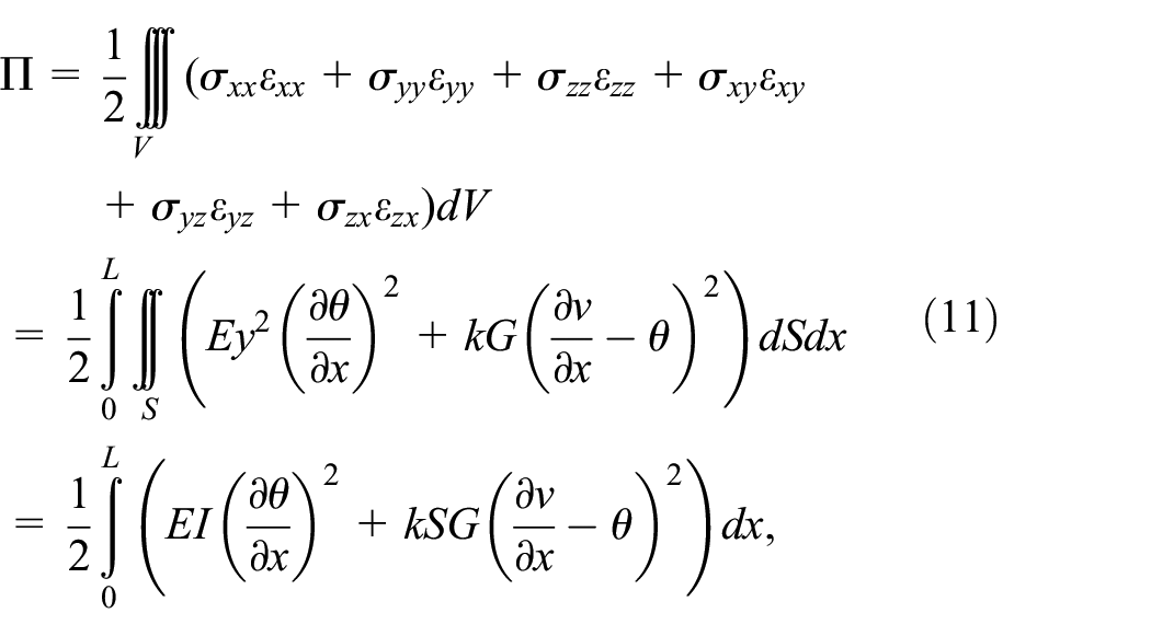
Now that the beam’s stress and strain values have been obtained, the kinetic and strain energy values can be achieved using the existing relations, and then the equations for the beam vibrations will be available using Hamilton’s principle. Note if the beam’s boundary conditions, properties, or additional forces change, so does the ultimate equation of motion. Here a beam with constant uniform properties, clamped on one side and free on the other, under no force, is examined. In the first step for strain energy (Π), when L is the length, and S is the surface, and I is the moment of inertia of the beam, we have:

$$\begin{array}{c}\mathrm{\Pi }=\frac{1}{2}\underset{V}{\int \int \int }({\sigma }_{\mathrm{xx}}{\epsilon }_{\mathrm{xx}}+{\sigma }_{\mathrm{yy}}{\epsilon }_{\mathrm{yy}}+{\sigma }_{\mathrm{zz}}{\epsilon }_{\mathrm{zz}}+{\sigma }_{\mathrm{xy}}{\epsilon }_{\mathrm{xy}}\hfill \\ \multicolumn{1}{c}{+{\sigma }_{\mathrm{yz}}{\epsilon }_{\mathrm{yz}}+{\sigma }_{\mathrm{zx}}{\epsilon }_{\mathrm{zx}})\mathrm{dV}}\\ =\frac{1}{2}\underset{0}{\overset{L}{\int }}\int \underset{S}{\int }(E{y}^2{\left(\frac{\partial \theta }{\partial x}\right)}^2+\mathrm{kG}{(\frac{\partial v}{\partial x}-\theta )}^2)\mathrm{dSdx}\hfill \\ =\frac{1}{2}\underset{0}{\overset{L}{\int }}(\mathrm{EI}{\left(\frac{\partial \theta }{\partial x}\right)}^2+\mathrm{kSG}{(\frac{\partial v}{\partial x}-\theta )}^2)\mathrm{dx},\hfill \end{array}$$

(11)

Moreover, the kinetic energy results from the beam’s transverse displacement in the period of the beam is (ρ is the beam’s density):

$$T=\frac{1}{2}\underset{0}{\overset{L}{\int }}(\rho S{\left(\frac{\partial v}{\partial t}\right)}^2+\rho I{\left(\frac{\partial \theta }{\partial t}\right)}^2)\mathrm{ds},$$

(12)

Applying Hamilton’s principle and using equations (11) and (12), the following relation is formed:

$$\begin{array}{c}\underset{t_1}{\overset{t_2}{\int }}(\mathrm{\Pi }-T-W)\mathrm{dt}=0,\hfill \\ \underset{t_1}{\overset{t_2}{\int }}[\underset{0}{\overset{L}{\int }}(\mathrm{EI}\frac{\partial \theta }{\partial x}\delta \left(\frac{\partial \theta }{\partial x}\right)+\mathrm{kSG}(\frac{\partial v}{\partial x}-\theta )\delta \left(\frac{\partial v}{\partial x}\right)\hfill \\ \multicolumn{1}{c}{-\mathrm{kSG}(\frac{\partial v}{\partial x}-\theta )\delta \theta )\mathrm{dx}-}\\ \underset{0}{\overset{L}{\int }}(\rho S\frac{\partial v}{\partial t}\delta \left(\frac{\partial v}{\partial t}\right)+\rho I\frac{\partial \theta }{\partial t}\delta \left(\frac{\partial \theta }{\partial t}\right))\mathrm{dx}-\underset{0}{\overset{L}{\int }}f\delta \mathrm{vdx}]\mathrm{dt}=0,\hfill \end{array}$$

(13)

Since no force is applied to the beam, the work done is equal to zero. By using the fractional integration method, equation (13) can give us the equations of motion of the beam in v and θ values:

$$-\frac{\partial }{\partial x}\left[\mathrm{kSG}(\frac{\partial v}{\partial x}-\theta )\right]+\rho S\frac{{\partial }^{2}v}{\partial t^2}=f(x,t),$$

(14)

$$-\frac{\partial }{\partial x}(\mathrm{EI}\frac{\partial \theta }{\partial x})-\mathrm{kSG}(\frac{\partial v}{\partial x}-\theta )+\rho I\frac{{\partial }^2\theta }{\partial t^2}=0,$$

(15)

The boundary conditions for the beam are:

$${\mathrm{kSG}(\frac{\partial v}{\partial x}-\theta )\delta v|}_0^L=0,{\mathrm{EI}\frac{\partial \theta }{\partial x}\delta \theta |}_0^L=0,$$

(16)

We are able to transform the two equations of motion into one fourth-order differential equation. In order to achieve this goal, equation (14) should be reformed as the following equations:

$$\begin{array}{c}-\mathrm{kSG}\frac{{\partial }^{2}v}{\partial x^2}+\mathrm{kSG}\frac{\partial \theta }{\partial x}+\rho S\frac{{\partial }^{2}v}{\partial t^2}=f,\hfill \\ \frac{\partial \theta }{\partial x}=\frac{{\partial }^{2}v}{\partial x^2}-\frac{\rho }{\mathrm{kG}}\frac{{\partial }^{2}v}{\partial t^2}+\frac{f}{\mathrm{kSG}},\hfill \end{array}$$

(17)

by deriving the equation (15) with respect to x, we have the relation below:

$$-\mathrm{EI}\frac{{\partial }^2}{\partial x^2}\left(\frac{\partial \theta }{\partial x}\right)-\mathrm{kSG}\frac{{\partial }^{2}v}{\partial x^2}+\mathrm{kSG}\frac{\partial \theta }{\partial x}+\rho I\frac{{\partial }^2}{\partial t^2}\left(\frac{\partial \theta }{\partial x}\right)=0,$$

(18)

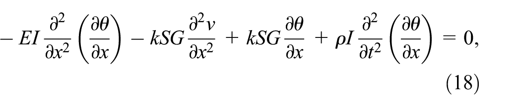
Finally, by replacing the modified form of the first equation (equation (17)) in equation (18), we will obtain the free vibration equation of a Timoshenko beam:

$$\mathrm{EI}\frac{{\partial }^{4}v}{\partial x^4}+\rho S\frac{{\partial }^{2}v}{\partial t^2}-\rho I(1+\frac{E}{\mathrm{kG}})\frac{{\partial }^{4}v}{\partial x^2\partial t^2}+\frac{{\rho }^{2}I}{\mathrm{kG}}\frac{{\partial }^{4}v}{\partial t^4}=0,$$

(19)

Obviously, the first two terms of equation (19) are like the first two terms of Euler-Bernoulli’s theory for beams, and the third and fourth terms represent the shear effect that do not exist in Euler-Bernoulli’s theory. We used a standard material for analyzing the Timoshenko beam, which is AISI 1020 steel. The properties of the mentioned material are shown in Table 1.

Table 1.

Properties of AISI 1020 steel.

Property	Value	Unit
Elastic modulus	2 × 1011	N/m2
Poisson’s ratio	0.29	—
Shear modulus	7.7 × 1010	N/m2
Mass density	7900	kg/m3
Tensile strength	420,507,000	N/m2
Yield strength	351,571,000	N/m2

Timoshenko’s beam’s equations of motion were solved by the finite element method, which brings us the beam displacement and the natural frequencies. In the first step of analyzing three different shapes, the first three iterations of Koch snowflakes (the first iteration is a simple triangle, the second iteration is a hexagram, and the third iteration) were considered as cross-sections (Figure 2). These three cross-sections have distinct geometry, area, and moment of inertia, which cause a different beam response. In the second step, the use of a hollow cross-section instead of solid was investigated. In the third step, the effect of four different boundary conditions on the beam’s behavior was examined. Table 2 illustrates the boundary conditions and their related equations.

Figure 2.

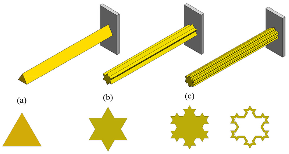
First three iteration of Koch snowflake as Timoshenko beam cross-sections: (a) first iteration (triangle), (b) second iteration (hexagram), and (c) third iteration.

Table 2.

Boundary condition and related equations.

Boundary condition type	Governing equations
Clamped	$v=0,\theta =0,$
Hinged	$v=0,\mathrm{EI}\frac{\partial \theta }{\partial x}=0,$
Free	$\mathrm{kSG}(\frac{\partial v}{\partial x}-\theta )=0,\mathrm{EI}\frac{\partial \theta }{\partial x}=0,$

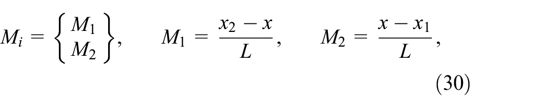
In the last step, beam properties such as density and modulus of elasticity were considered variable along the beam. The density and elastic modulus equations are shown in equations (20) and (21), respectively.

$$\begin{array}{c}\multicolumn{1}{c}{E(x)=(E_L-E_R){\left(\frac{x}{L}\right)}^{1.5}+E_L,E_L=70\times {10}^{9}N/m^2,}\\ \multicolumn{1}{c}{E_R=200\times {10}^{9}N/m^2,}\end{array}$$

(20)

$$\begin{array}{c}\multicolumn{1}{c}{\rho (x)=({\rho }_L-{\rho }_R){\left(\frac{x}{L}\right)}^{1.5}+{\rho }_L,{\rho }_L=2700\mathrm{kg}/m^3,}\\ \multicolumn{1}{c}{{\rho }_R=7900\mathrm{kg}/m^3,}\end{array}$$

(21)

Finite element method (FEM)

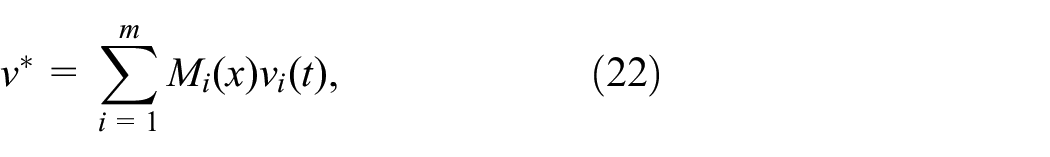
The equation of motion (equation (19)) of the Timoshenko beam was solved by the finite element method (FEM) by using MATLAB software. Here is a summary of the procedure of FEM.^32–35 In the beginning, we have to determine the properties, area, and moment of inertial for each cross-section, which directly affects the beam’s stiffness and mass matrices. After that, we need to indicate the number of nodes, elements, and the shape function to solve the problem. So, 50 elements with 51 nodes, and that the length of the elements is considered equal. The total number of degrees of freedom is 102, which is twice the number of nodes. With these establishments, we introduce v* and θ* in element {e} as the shape functions for v and θ functions, respectively:

$$v^{*}=\sum _{i=1}^m{M}_i(x)v_i(t),$$

(22)

$${\theta }^{*}=\sum _{i=1}^m{N}_i(x){\theta }_i(t),$$

(23)

In calculating the stiffness and mass matrices in each element, shear force and bending effects are considered separately. Then we substitute the v* and θ* in equations (14) and (15) to obtain the residues. Based on the standard Galerkin technique, the residues are made orthogonal with respect to the shape functions, so for each element, we have:

$${\int }_V[-\frac{\partial }{\partial x}\left[\mathrm{kSG}(\frac{\partial v^{*}}{\partial x}-{\theta }^{*})\right]+\rho S\frac{{\partial }^2{v}^{*}}{\partial t^2}-f(x,t)]M_i\mathrm{dx}=0,$$

(24)

$$\begin{array}{c}\multicolumn{1}{c}{{\int }_V[-\frac{\partial }{\partial x}\left(\mathrm{EI}\frac{\partial {\theta }^{*}}{\partial x}\right)-\mathrm{kSG}(\frac{\partial v^{*}}{\partial x}-{\theta }^{*})+\rho I\frac{{\partial }^2{\theta }^{*}}{\partial t^2}]}\\ \multicolumn{1}{c}{N_i\mathrm{dx}=0,}\end{array}$$

(25)

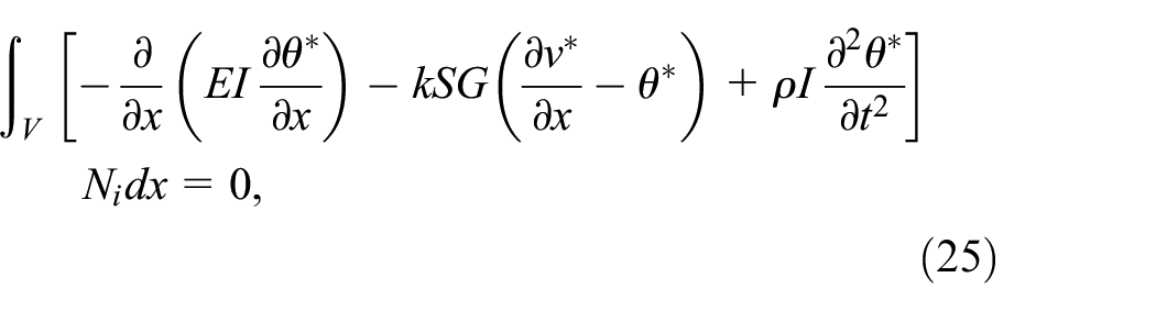
By weak formulation for the terms ∂²v*/∂x² and ∂²θ*/∂x² and replacing the shape function in the equations (24) and (25), when no external force is applied to the beam, we achieve the following relations:

$$\begin{array}{c}\multicolumn{1}{c}{m\frac{{\partial }^2{v}_j}{\partial t^2}\underset{0}{\overset{L}{\int }}{M}_j{M}_i\mathrm{dx}+\mathrm{kSG}{v}_j\underset{0}{\overset{L}{\int }}\frac{d{M}_j}{\mathrm{dx}}\frac{d{M}_i}{\mathrm{dx}}\mathrm{dx}}\\ \multicolumn{1}{c}{-\mathrm{kSG}{\theta }_j\underset{0}{\overset{L}{\int }}\frac{d{M}_i}{\mathrm{dx}}\mathrm{dx}={\mathrm{kSG}\frac{\partial v^{*}}{\partial x}{M}_i|}_0^L+{\mathrm{KSG}{\theta }^{*}{N}_i|}_0^L,}\end{array}$$

(26)

$$\begin{array}{c}\multicolumn{1}{c}{J\frac{{\partial }^2{\theta }_j}{\partial t^2}\underset{0}{\overset{L}{\int }}{N}_j{N}_i\mathrm{dx}+\mathrm{EI}{\theta }_j\underset{0}{\overset{L}{\int }}\frac{d{N}_j}{\mathrm{dx}}\frac{d{N}_i}{\mathrm{dx}}\mathrm{dx}+\mathrm{kSG}{\theta }_j\underset{0}{\overset{L}{\int }}{N}_j{N}_i\mathrm{dx}}\\ \multicolumn{1}{c}{-{\mathrm{kSG}{v}_j\underset{0}{\overset{L}{\int }}\frac{d{M}_j}{\mathrm{dx}}{N}_i\mathrm{dx}=\mathrm{EI}\frac{\partial {\theta }^{*}}{\partial x}{N}_i|}_0^L.}\end{array}$$

(27)

For all elements and nodes of the beam, equations (26) and (27) in the matrix form are:

$$\left[m\right]\left\{\frac{{\partial }^{2}v}{\partial t^2}\right\}+\left[K_1\right]\left\{v\right\}+\left[K_2\right]\left\{\theta \right\}=\left\{F_1\right\}+\left\{F_1^{\mathrm{BC}}\right\},$$

(28)

$$\left[J\right]\left\{\frac{{\partial }^2\theta }{\partial t^2}\right\}+\left[K_3\right]\left\{\theta \right\}+\left[K_4\right]\left\{v\right\}=\left\{F_2^{\mathrm{BC}}\right\},$$

(29)

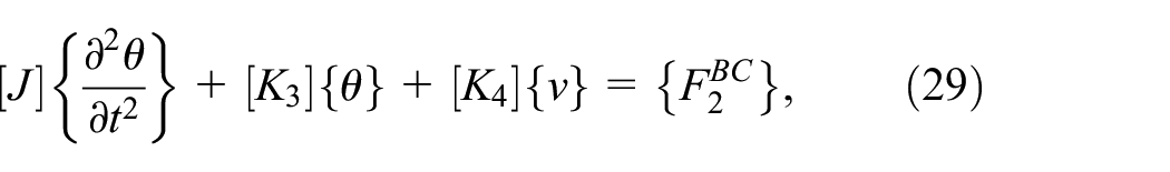
Utilizing the appropriate procedure for the solution, equations (28) and (29) are solved in the time domain for desired initial conditions. To solve the problem in the x domain, we consider linear shape functions for the unknown variables:

$$M_i=\left\{\begin{array}{c}{M}_1\hfill \\ \multicolumn{1}{c}{M_2}\end{array}\right\},M_1=\frac{x_2-x}{L},M_2=\frac{x-x_1}{L},$$

(30)

$$N_i=\left\{\begin{array}{c}{N}_1\hfill \\ \multicolumn{1}{c}{N_2}\end{array}\right\},N_1=\frac{x_2-x}{L},N_2=\frac{x-x_1}{L},$$

(31)

By applying the shape functions, the matrices for mass can be calculated:

$${\left[m\right]}_{\mathrm{ij}}^e=m\underset{0}{\overset{L}{\int }}\left[\begin{array}{c}{M}_1^2{M}_1{M}_2\hfill \\ \multicolumn{1}{c}{M_1{M}_2{M}_2^2}\end{array}\right]\mathrm{dx}=\frac{\mathrm{mL}}{6}\left[\begin{array}{cc}2\hfill & 1\hfill \\ \multicolumn{1}{c}{1}& 2\hfill \end{array}\right],$$

(32)

$${\left[J\right]}_{\mathrm{ij}}^e=J\underset{0}{\overset{L}{\int }}\left[\begin{array}{c}{N}_1^2{N}_1{N}_2\hfill \\ \multicolumn{1}{c}{N_1{N}_2{N}_2^2}\end{array}\right]\mathrm{dx}=\frac{\mathrm{JL}}{6}\left[\begin{array}{cc}2\hfill & 1\hfill \\ \multicolumn{1}{c}{1}& 2\hfill \end{array}\right],$$

(33)

And for the element stiffness matrices, we have:

$$\begin{array}{c}{\left[K_1\right]}_{\mathrm{ij}}^e=\mathrm{kSG}\underset{0}{\overset{L}{\int }}\left[\begin{array}{c}\frac{d{M}_1}{\mathrm{dx}}\frac{d{M}_1}{\mathrm{dx}}\frac{d{M}_1}{\mathrm{dx}}\frac{d{M}_2}{\mathrm{dx}}\hfill \\ \multicolumn{1}{c}{\frac{d{M}_2}{\mathrm{dx}}\frac{d{M}_1}{\mathrm{dx}}\frac{d{M}_2}{\mathrm{dx}}\frac{d{M}_2}{\mathrm{dx}}}\end{array}\right]\mathrm{dx}=\frac{\mathrm{kSG}}{L}\left[\begin{array}{cc}1\hfill & -1\hfill \\ \multicolumn{1}{c}{-1}& 1\hfill \end{array}\right],\hfill \\ {\left[K_2\right]}_{\mathrm{ij}}^e=\mathrm{kSG}\underset{0}{\overset{L}{\int }}\left[\begin{array}{c}\frac{d{M}_1}{\mathrm{dx}}{N}_1\frac{d{M}_1}{\mathrm{dx}}{N}_2\hfill \\ \multicolumn{1}{c}{\frac{d{M}_2}{\mathrm{dx}}{N}_1\frac{d{M}_2}{\mathrm{dx}}{N}_2}\end{array}\right]\mathrm{dx}=\frac{\mathrm{kSG}}{2}\left[\begin{array}{cc}-1\hfill & -1\hfill \\ \multicolumn{1}{c}{1}& 1\hfill \end{array}\right],\hfill \\ {\left[K_3\right]}_{\mathrm{ij}}^e=\mathrm{EI}\underset{0}{\overset{L}{\int }}\left[\begin{array}{c}\frac{d{N}_1}{\mathrm{dx}}\frac{d{N}_1}{\mathrm{dx}}\frac{d{N}_1}{\mathrm{dx}}\frac{d{N}_2}{\mathrm{dx}}\hfill \\ \multicolumn{1}{c}{\frac{d{N}_2}{\mathrm{dx}}\frac{d{N}_1}{\mathrm{dx}}\frac{d{N}_2}{\mathrm{dx}}\frac{d{N}_2}{\mathrm{dx}}}\end{array}\right]\mathrm{dx}-\mathrm{kSG}\underset{0}{\overset{L}{\int }}\left[\begin{array}{c}{N}_1^2{N}_1{N}_2\hfill \\ \multicolumn{1}{c}{N_1{N}_2{N}_1^2}\end{array}\right]\hfill \\ \mathrm{dx}=\frac{\mathrm{EI}}{L}\left[\begin{array}{cc}1\hfill & -1\hfill \\ \multicolumn{1}{c}{-1}& 1\hfill \end{array}\right]-\frac{\mathrm{kSGL}}{6}\left[\begin{array}{cc}2\hfill & 1\hfill \\ \multicolumn{1}{c}{1}& 2\hfill \end{array}\right],\hfill \\ {\left[K_4\right]}_{\mathrm{ij}}^e=\mathrm{kSG}\underset{0}{\overset{L}{\int }}\left[\begin{array}{c}{N}_1\frac{d{M}_1}{\mathrm{dx}}{N}_1\frac{d{M}_2}{\mathrm{dx}}\hfill \\ \multicolumn{1}{c}{N_2\frac{d{M}_1}{\mathrm{dx}}{N}_2\frac{d{M}_2}{\mathrm{dx}}}\end{array}\right]\mathrm{dx}=\frac{\mathrm{kSG}}{2}\left[\begin{array}{cc}-1\hfill & -1\hfill \\ \multicolumn{1}{c}{1}& 1\hfill \end{array}\right].\hfill \end{array}$$

(34)

Finally, the system of equation for the element {e} is formed:

$$\left[\overline{M}\right]\left\{\stackrel{··}{X}\right\}+\left[\overline{K}\right]\left\{X\right\}=\left\{\overline{F}\right\},\left\{X\right\}=\left\{\begin{array}{c}{v}_1\hfill \\ \multicolumn{1}{c}{{\theta }_1}\\ \multicolumn{1}{c}{v_2}\\ \multicolumn{1}{c}{{\theta }_2}\end{array}\right\}.$$

(35)

It should be noted that solving this equation will be correct when the boundary conditions are applied correctly in the problem. In the end, the displacement function according to the nodes in the beam length will be obtained.

Result and discussion

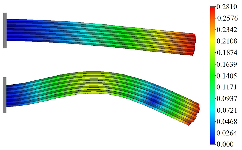
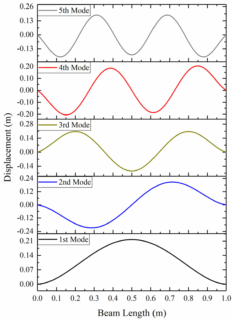
After finding the equation of motion for the Timoshenko beam and solving the problem using the finite element method, we analyzed it in different conditions. The first three iterations of the Koch snowflake are considered as cross-sections in the first analysis. Figures 3 to 5 show the beam’s first five mode shape for each cross-section in the clamped-free boundary condition. However, to validate our result, Solidworks simulation, an alternative for time-consuming FEA software, is used, which has been used in previous studies.^36,37 Figures 6 to 9 illustrate the first two modes of each cross-section in Solidworks simulation. It can be seen that the maximum error for displacement is 0.3 %, 0.3%, and 0.36% for the first mode, and about 2.92%, 2.85%, and 2.87% for the second mode, for the first three iterations, respectively, which proves that the applied method has acceptable accuracy. Furthermore, each mode’s corresponding natural frequency for every cross-section compared to Solidworks simulation is illustrated in Tables 3 to 5. The maximum errors between all mode shapes are about 2.96%, 1.97%, and 2.61% for the first three iterations of Koch snowflake for frequencies.

Figure 3.

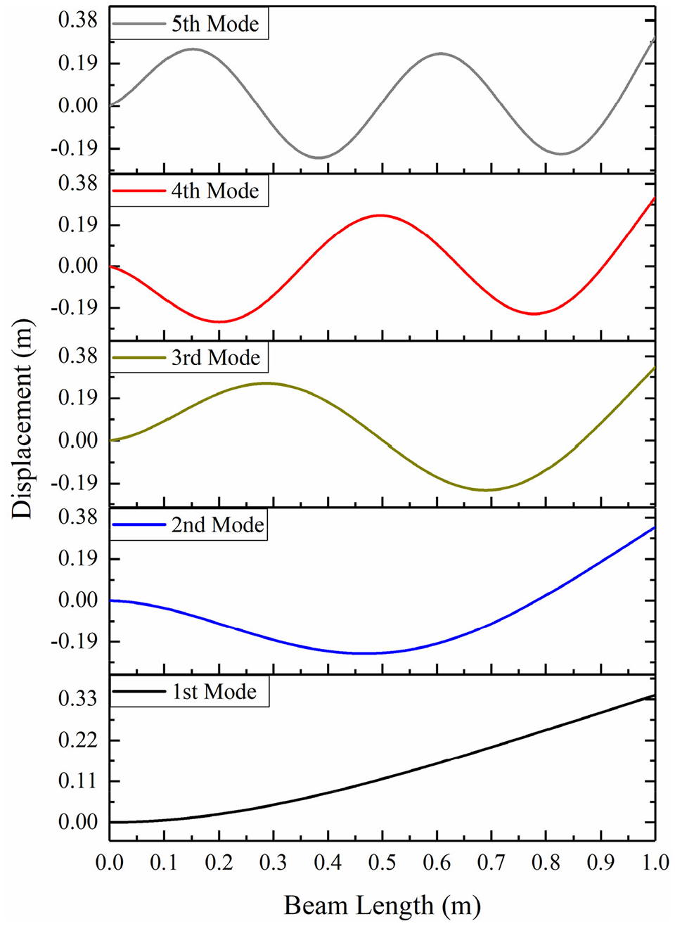
Mode shape of the beam for the first iteration of Koch snowflake (triangle) cross-section.

Figure 4.

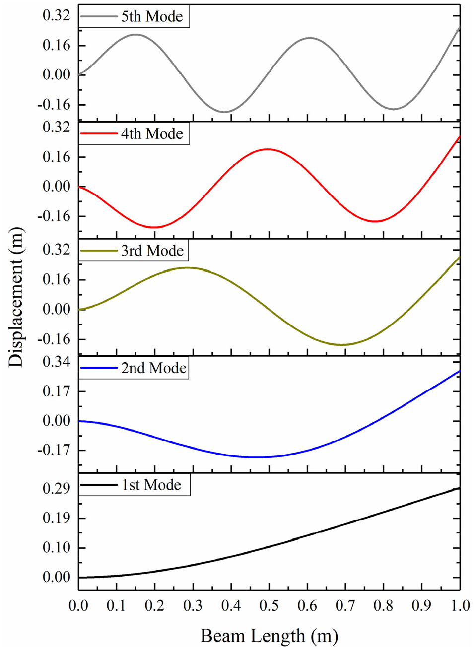
Mode shape of the beam for the second iteration of Koch snowflake (hexagram) cross-section.

Figure 5.

Mode shape of the beam for the third iteration of Koch snowflake cross-section.

Figure 6.

First and second mode shape for triangle cross-section in simulation.

Figure 7.

First and second mode shape for hexagram cross-section in simulation.

Figure 8.

First and second mode shape for Koch snowflake cross-section in simulation.

Figure 9.

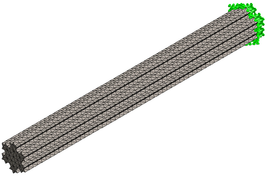
Mesh of the Timoshenko beam with Koch snowflake cross-section in the clamped-free boundary condition.

Table 3.

Comparison of natural frequency for FEM and Solidworks simulation for the first iteration of Koch snowflake (triangle) cross-section (rad/s).

Modenumber	FEM	Solidworkssimulation	Error(%)
1st	364.4088	360.76	1.0114
2nd	2233.7223	2205.20	1.2934
3rd	6052.4052	5949.70	1.7262
4th	11,357.8218	11,357.00	0.0072
5th	17,868.0771	17,355.00	2.9564

Table 4.

Comparison of natural frequency for FEM and Solidworks simulation for the second iteration of Koch snowflake (hexagram) cross-section (rad/s).

Modenumber	FEM	SolidworksSimulation	Error (%)
1st	401.5833	398.64	0.7383
2nd	2449.7397	2427.60	0.9120
3rd	6593.8871	6516.80	1.1829
4th	12,276.9410	12,090.00	1.5462
5th	19,161.5002	18,791.00	1.9717

Table 5.

Comparison of natural frequency for FEM and Solidworks simulation for the third iteration of Koch snowflake cross-section (rad/s).

Modenumber	FEM	Solidworkssimulation	Error (%)
1st	422.6378	419.87	0.6592
2nd	2570.6686	2546.00	0.9689
3rd	6892.3943	6795.80	1.4214
4th	12,774.7966	12,525.00	1.9944
5th	19,850.3826	19,345.00	2.6125

From a vibrational point of view, in each iteration level for cross-section, the area, and moment of inertia increase, which cause the higher natural frequency in a mode. The rise in areas are 33.33% and 11.11%, and the increase in the moment of inertia are 62.96% and 23.46% at each level. Simultaneously, the natural frequency increased by 10.2% and 5.24% for the first mode shape.

It should be mentioned that in the Solidworks simulation, mesh type was considered solid, and four Jacobina points were selected. 11,947 and 20,662 are the number of elements and nodes, so each element size is equal to 21.3716 mm. Timoshenko beam meshing with the third iteration of Koch snowflake cross-section with clamped-free boundary condition is shown in Figure 9.

Next, the hollow cross-section effect in the displacement and natural frequency of the beam is investigated. The mode shapes of this cross-section are shown in Figure 10. The area and moment of inertia in the hollow cross-section compared to solid one has decreased about 63.83% and 41.44%; in contrast, the natural frequency growth is approximately 26.37%. This phenomenon is happed because natural frequency has a direct relationship with stiffness and an inverse relationship with mass, and in this case, the mass of the beam has reduced. Figure 11 shows a comparison for the natural frequencies in the first five mode shapes for the three iterations of Koch snowflake and hollow cross-section.

Figure 10.

Mode shape of the beam for hollow Koch snowflake cross-section.

Figure 11.

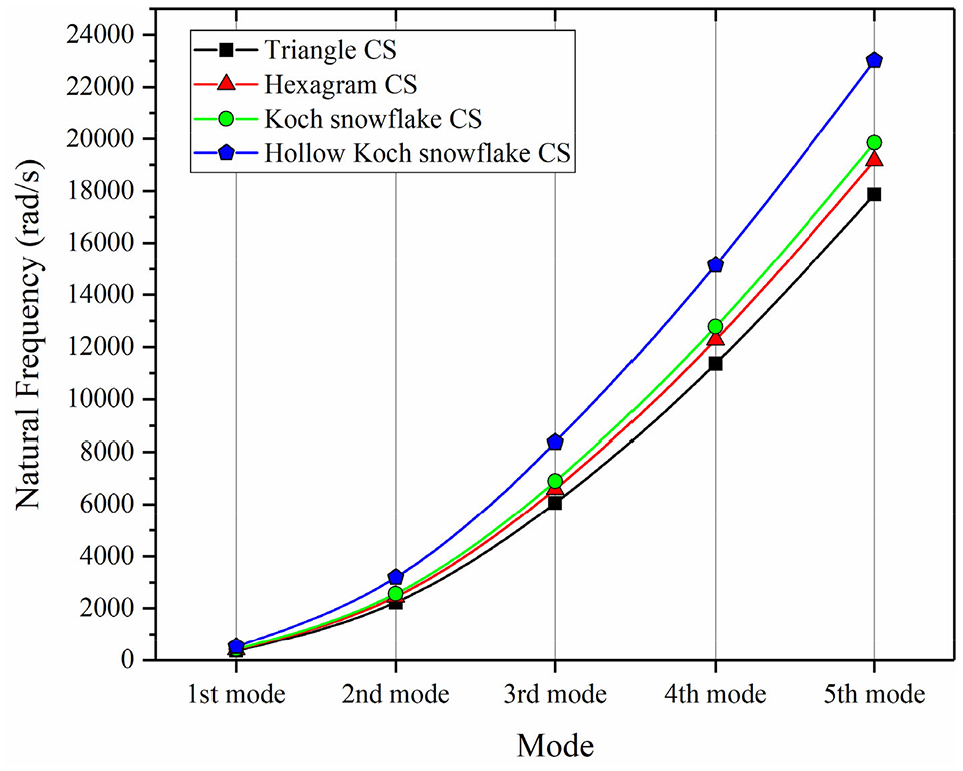
Comparison of natural frequencies for different cross-sections.

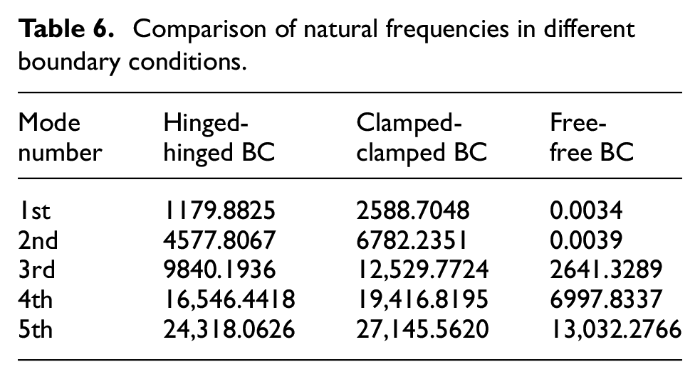
The behavior of any beam is under the influence of boundary conditions. ³⁸ So, for the Timoshenko beam, we studied it under the clamped-free, clamped-clamped, hinged-hinged, and free-free boundary conditions with the relation in Table 2. Figures 12 to 14 demonstrate the beam’s displacement for different states, where we can see that the slope of the beam’s displacement near both ends changes while the max amplitude is approximately constant for every condition. Table 6 shows the natural frequency of each mode for all conditions. Natural frequencies for the clamped-clamped boundary condition are highest, free-free boundary conditions are lowest, and hinged-hinged is placed in the middle.

Figure 12.

Mode shape of the beam for Koch snowflake cross-section with clamped-clamped boundary condition.

Figure 13.

Mode shape of the beam for Koch snowflake cross-section with hinged-hinged boundary condition.

Figure 14.

Mode shape of the beam for Koch snowflake cross-section with free-free boundary condition.

Table 6.

Comparison of natural frequencies in different boundary conditions.

Mode number	Hinged-hinged BC	Clamped-clamped BC	Free-free BC
1st	1179.8825	2588.7048	0.0034
2nd	4577.8067	6782.2351	0.0039
3rd	9840.1936	12,529.7724	2641.3289
4th	16,546.4418	19,416.8195	6997.8337
5th	24,318.0626	27,145.5620	13,032.2766

Figures 15 and 16 illustrate the Timoshenko beam’s mode shape when density and elastic modulus vary along the beam. Under the function in equations (20) and (21), density and elastic modulus change along the beam from a minimum value to the standard value. Table 7 shows the natural frequencies for the beam with variable properties. It is understandable from Table 7 that variable density has increased the frequency while the variable elastic modulus declined it.

Figure 15.

Mode shape of the beam for Koch snowflake cross-section with variable density.

Figure 16.

Mode shape of the beam for Koch snowflake cross-section with variable elastic modulus.

Table 7.

Natural frequencies for variable density and elastic modulus.

Mode number	Variabledensity	Variable elasticmodulus
1st	465.2849	269.7000
2nd	3199.9036	1842.4068
3rd	8919.7376	5106.2310
4th	16,676.7977	9522.1248
5th	25,992.5532	14,823.0343

Conclusion

This study analyzed a beam with the cross-section of the first three Koch snowflake iterations with Timoshenko Theory. The governing equation of the beam was solved by the finite element method and was verified by simulation. The behavior of the beam under the variable properties and different geometries and boundary conditions were studied, and the significant results are as follow:

• In each level of Koch snowflake iteration used as a cross-section, the area and moment of inertia increase, and it causes a 5.2% and 10.2%, and 5.24% rise in the first natural frequency.

• Hollow Koch snowflake cross-section can enlarge the natural frequency by about 26.37% compared to a solid one.

• Change in boundary conditions changes the slope of the beam’s displacement in the ends. Moreover, the clamped-clamped, hinged-hinged, clamped-free, and free-free have the highest natural frequency for the Timoshenko beam with Koch’s third iteration snowflake cross-section.

• Variable density from a minimum value to the standard value along the beam increases the natural frequency, while variable elastic modulus decreases.