
Abstract
The manufacture of total hip arthroplasty (THA) requires the control of the quality of free form surfaces. In fact, the polyethylene insert is deformed to fit the overall geometry of the femoral part, which has an impact on the quality of the contact. In this paper, we propose a method for evaluating the defects of complex forms. The originality of the approach is the use of artificial intelligence to position the cloud of measured points, obtained with a three-dimensional measuring machine equipped with a contactless sensor, with regard to the 3D CAD model of the THA. The artificial intelligence algorithm used is based on neural networks that are trained using a virtual positioning realized with 3D CAD software. Finally, the difference between the positioned point cloud and the CAD model allows us to evaluate the shape defect of the measured THA surface. We found that the error of the proposed method is at the vicinity of micron scale.
Introduction
Total hip arthroplasty (THA) provides momentous enhancement in mobility and quality of life for patients suffering from osteoarthritis of the hip. Lan et al. 1 reported that an increase in THA by 71% toward 635,000 procedures per year, by 2030 is projected. As the occurrence of osteoarthritis and the procedure volumes of THA continue to raise, mastery of their manufacturing quality control is required. Indeed, the control of the form defects of the THA surface is crucial to ensure the proper functioning of the complete system. The contact between the femoral component (cobalt-chromium alloy head and femoral stem) and the cup of hip (polyethylene part) are illustrated in Figure 1. The acceptable defect must guarantee the femoral head/cup contact of hip stability and the amplitude of the geometrical defect between these two components must not induce a risk of wear. Coordinate measuring machine (CMM) is one of the most common in vitro wear measure methods. 2 In this context, 3 investigated the evaluation of hip implant wear measurements by analyzing acetabular components in polyethylene using CMM technique and showed that identifying key elements of the measurement uncertainty are crucial to enhance the reliability and the accuracy of CMM wear measurement. The CMM generated data points (3D point cloud) were exported to a text file and imported into computer-aided design (CAD) software in order to determine the diameter of the explanted femoral heads by creating two spheres to simulate the position of the femoral head in the cup. 4 While Dall’Ava et al., 5 measured the internal and external diameter of the off-the-shelf cup by scanning the internal and external surface near the edge of the cup with an average of 14,500 points for each of the five trace treated. The CMM software automatically computed the values of the diameters.

Diagram of total hip implant. 6
Research on the analysis of free form surfaces defect realized by comparing a nominal mathematical model with a measured point cloud, obtained from a three-dimensional non-contact measuring machine, was investigated since the eighties. 7
Ip and Gupta 8 used partial 3D point cloud of an artifact for retrieving the CAD model of the object. Adopting the assumption that the point clouds are evenly sampled on the target surface, they proposed a three step approach: first, partially scanned point clouds and polygonal CAD meshes (CAD models) are separated into surface patches, afterwards aligned and compared according to the main components of the surface patches. The matching of scanned point cloud to CAD meshes approach consists of three stages: (i) segmentation of point cloud and CAD models into surface patches using an identical algorithm, (ii) identification of the matching patches in point cloud and CAD models, and finally (iii) aligning the point cloud with the CAD models and evaluating the error associated with the alignment.
In recent years, scholars have done several researches on the registration problem, that is the proper localization of the 3D point clouds, like those originated by CMMs and structured light scanners, in the same coordinate system. Pauwels 9 stated that for fine registration known variants of the Iterative Closest Point (ICP) algorithm are commonly implemented and investigated an original approach that targets multisensor coordinate metrology scenarios specific issues. The proposed approach is based on joining implementation of the ICP and point augmentation algorithms. It was concluded that even the best ICP solution would greatly benefit from an supplementary step consisting in processing the data sets to be registered, specifically, processing the fixed point set by point augmentation.
Future intelligent three-coordinate measuring machines has attracted the attention of Han et al. 10 who proposed a T-spline based unifying registration technique for free-form surface artifact in intelligent CMM. While artificial intelligence approach to free-form shapes registration has been investigated by several others scholars. Kang et al. 11 proposed the use of a data-driven deep learning methodology to automatically detect and classify building elements constructed form a laser-scanned point cloud scene. Kang et al. 11 work is based on three steps. First, the points cloud is converted into a graph representation (where vertices represent points and edges represent connections between points inside a fixed distance). Next, the type of building component is determined based on the segmented points and augmented with context from nearby points. Finally, each identified object is matched with a corresponding building information model entity based on the nearest neighbor in the feature space. An edge-based classifier was used in the first step while in the second one a point-based object classifier was employed. The issue of finding a procedure allowing positioning the measured point cloud with regard to the mathematical model has been explored. Different methods have been used, namely the least square method. 2 However, this latter does not guarantee the determination of the shape defect in the standard meaning because it is based on an optimization algorithm, which can converge to a local minimum. Artificial intelligence systems, developed since the early sixties, show their efficiency to evaluate geometric defects. 12 Therefore, it seems appropriate to use such tools to evaluate the form defects of prosthesis. Indeed, the shape of hip prostheses is complex because it associates several different free form surfaces. The analytical resolution of this problem leads to a nonlinear differential equations system of several variables. The resolution of these equations induces divergence errors. However, the exploitation of the neural network system makes it possible to do without complex mathematical resolutions. The issue is, therefore, to determine the relevant neural network application for positioning measured points with regard to a nominal 3D CAD model and to estimate form defects.
The aim of this work is, therefore, to propose a robust positioning method of measured points with regard to a CAD model for evaluating the shape defects of a free form surface.
Research assumptions and methodology
The problem is to find a method to position a cloud of points measured on the real surface with its theoretical model. In this study, we are interested in femoral stem implant I-Hip which is composed of forged alloy Ti-6Al-4V ELI. The stem is designed in double cones and has a slight symmetrical taper, proximal to distal, in the sagittal plane and an essentially symmetrical taper, proximal to distal, in the coronal plane, ending with a rounded tip. The proximal side path is bent to allow the rod to clean the bone base of the femoral greater trochanter during the insertion step.
The evaluation of the form defect of the produced femoral stem is done by comparing points measured on the produced part and the nominal 3D CAD model after a relevant positioning of the measured points. Thus, the present paper focus on the definition of a positioning method of the measured points with regard to the nominal 3D CAD model using artificial intelligence algorithm of the neural network type. The problem is to propose a suitable neural network as well as its learning protocol to define this positioning method. The knowledge of the produced defects must make it possible to set up the manufacturing process to improve the produced quality. With reference to the methods of association (adaptation) to the point cloud model taken by a non-contact probe, which we will have exposed among the most used for the three-dimensional case. The method of association is small displacements which imposes the use of a local reference mark in order to obey the condition of the small displacements which limits its exploitation for clouds of points a little distant from the real surface, but with less complexity for processing by neural networks. The nonlinear method for its part theoretically offers the possibility of making an association between a cloud of points and a surface quite distant from each other, but the nonlinear nature of the problem in this case poses difficulties of stability and convergence. We have also seen some researchers who have explained the ICP method with a little detail and in addition to its nonlinear character, it is its simplicity which is very suitable for the chosen surface model, that is the STL model that we used. 1
Materials and methods
Cloud of hip prosthesis points
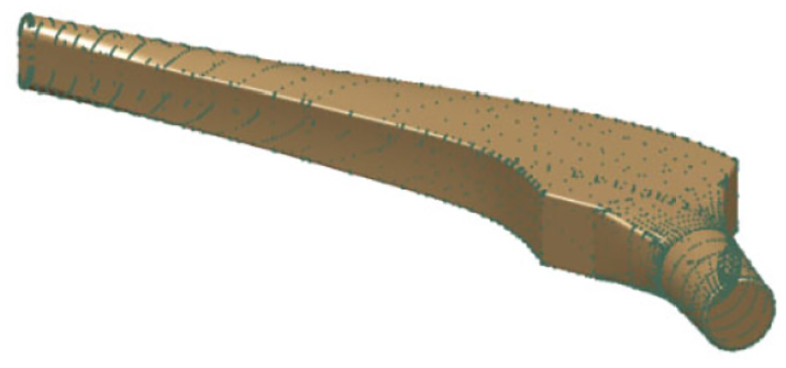
We use a three-dimensional measuring machine with Geomatic software to obtain the point cloud of the studied part. In our case, we get 6841 points coordinates in the Cartesian coordinate system of the measuring machine (x, y, z). These points are obtained using a contactless probe (Figure 2(a)).

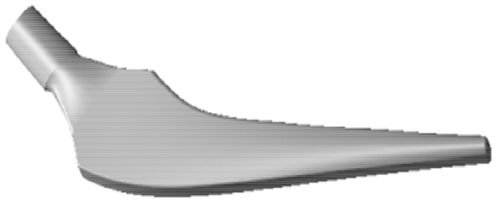
Acquisition of prosthesis geometric data to be analyzed: (a) cloud of points, (b) STL format file, and (c) 3D CAD prosthesis.
STL format of the hip prosthesis
The STL format is usually obtained by triangulating an exact model using CAD software. A STL data file is defined from triangular facets defined by the coordinates of the three vertices and its normal directed to the free side of the object. The 3D point cloud format conversion operation in STL format is performed by Catia V6 software. For the hip prosthesis the number of facets obtained is 13,678 (Figure 2(b)).
Design of the hip prosthesis
The femoral stem implant I-Hip is created and can be used to perform operations to obtain a part with a relevant quality 13 (Figure 2(c)).
Rapid THA prosthesis prototyping process
Rapid prototyping concerns all the technologies, that make it possible to obtain the physical representation of a 3D CAD model in a very short time. 14 This rapid prototyping relies on a set of tools that allow to achieve intermediate product representation projects: numerical models (product geometry), digital and physical models, prototypes, and pre-series. This system integrates three essential notions that are 14 :
Time: The purpose of rapid prototyping is to quickly realize models, with the aim of reducing product development time.
Cost: Rapid prototyping makes it possible to produce prototypes without the need for expensive tools, while guaranteeing the performance of the final product.
Shape complexity: The control of the produced geometrical defects still requires an experimental process based on the measurement of the realized part defects and the implementation of corrective action. Thus, this work can be included in a reverse engineering scheme (Figure 3).
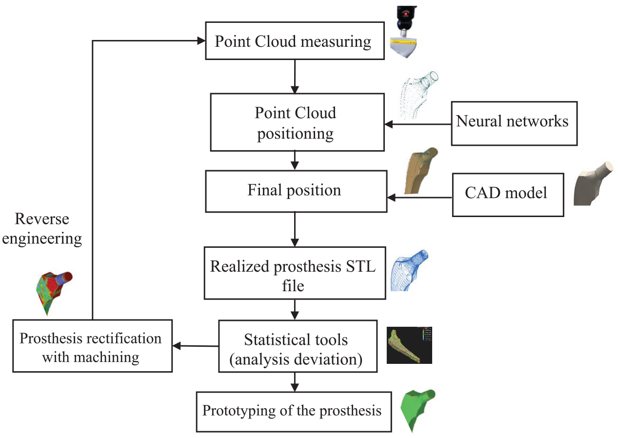
Organizational chart of the prosthesis prototyping.
Materials
The measuring instruments used in scientific research is a Surface Measure of type 606 of support PH10MQ probing probe type laser irradiation scanning error 12 µm, max acquisition rate 75,000 points/s, laser class 2 (JIS C 6802 2011), line laser wavelength 660 nm, points laser wavelength 635 nm. The software used is Catia V6 to process it’ information. This software is available from the research laboratory, UMR 6602 – UCA/CNRS/SIGMA.
The hip prosthesis parts are offered by Laboratory of Applied Biomechanics and Biomaterials (LABAB), ENP Oran (Algeria), with even the dimensions and the quality of the surface state (Figure 5).
Exploration of the neural networks method for the measured prosthesis positioning
A neural network model was applied for the positioning of the measured points with respect to the 3D CAD nominal model of the femoral stem. In input the neural network receives the three coordinates (xr, yr, zr) of each measured points in the measure coordinate system and in output, it calculates the three coordinates (xe, ye, ze) of the measured points in the 3D CAD coordinate system allowing the superposition of the point cloud with the 3D CAD nominal model. The neural network used is composed of 10 layers. The training of this network makes it possible to determine the magnitudes of the weights of the synapses of this model W, Z, G, w0, z0, and g0 (Figure 4).

Neural network identification.
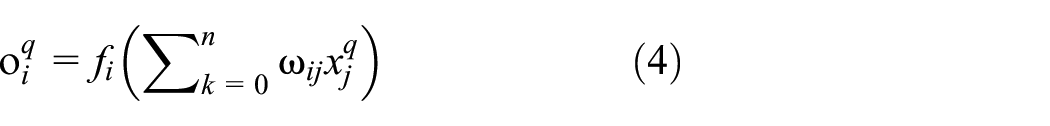
Presentation of the neural network model
The elements of the neural network are based on the exponential function (equation (1)) and a weighted summation of signals (x1r, y1r, z1r), (x2r, y2r, z2r), …, (x5r, y5r, z5r) as shown in Figure 4. The weighting coefficients ω i (i = 0, 1, …, n) are called synaptic points. If ωi is positive (xie, yie, zie) is the input excitement. When ωi is negative, it is inhibitory. In fact, to finalize the model, it is necessary to determine the parameters W, w0, Z, z0, G, g0 according to known output variables (xir, yir, zir).

Thus, to minimize E, we move proportionally to the negative of ∇E, leading to the updating of each weight ωjk as:


Recall that the gradient ∇E of E at a point ω with components ωij is the vector of partial derivatives

where

and η > 0 is a number called the learning rate.
We have


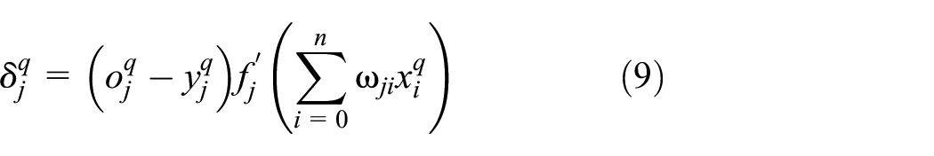
For the jth output neuron.
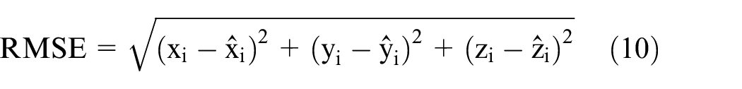
Root mean square error (RMSE)
The RMSE is another performance criterion frequently used which measures the difference between the values predicted by a model or an estimator and the actual observed values from a modeling or estimation (equation (2)). This error is deduced from the square root of the mean squared error, as shown in equation given below:
Databases definition for learning and validation of artificial neural networks
Three-dimensional Coordinate Measuring Machine (CMM) is used to obtain the coordinates of the measured points of a specimen in a measure coordinate system (Figure 5). Different test setups can be used which is the based to define the learning database of artificial intelligence.
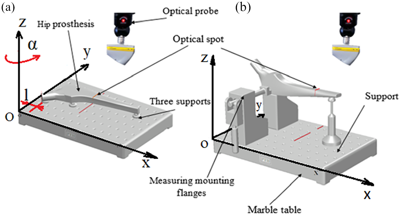
Measurement setup in the optical probe machine, (a) acquisition based (α, l), (b) acquisition in position adapted to the proposed model (α = 0, l = 0).
Before implementing the neural network positioning method, a learning phase must be performed. This phase is carried out using a setup (Figure 5(a) and (b)). The points are measured on the nominal CAD model by simulating the position of the measure setup in the measuring coordinate system (Figure 5(b)). The input of learning is this point cloud measured by simulating a measurement setup and the output is the initial position in the CAD.
Figure 6 shows the nominal prosthesis 3D model (in brown color). The points cloud of the measured prosthesis N° 1 (in green color) makes a rotation α = −45° with respect to the model coordinate system and a translation l = 0 mm according to the axes. This points cloud is composed of 6841 points. The second points cloud (Figure 7) is obtained with a virtual measurement setup like the one of Figure 5(a) (in green color). We find that the percentage of positioning of the points cloud on the model is more than 95% (Figure 7).

Point cloud of the hip prosthesis 1 such as α = −45° and translation l = 0 mm.

Point cloud of prosthesis 1 positioned on the model.
In the case of Figure 8 the points cloud of the measured prosthesis N° 2 (in green color) makes a rotation α = −20° with respect to the model and a translation equal to l = −2 mm according to the selected reference axes. The point cloud captured by the measuring machine are more than 10,000 points, but we did the filtering by software with outre calling this operation within our scientific work. The points cloud entered is composed of 6841. By obtaining, the second points cloud (Figure 9). We can see that the positioning percentage is more than 99.10%. For Figures 9 and 10 the points cloud of the measured prosthesis N° 3 (in green color) makes a rotation α = +10° with respect to the model and a translation equal to l = 3 mm. The point cloud is composed of 5841 points. By obtaining the second measured points cloud in the new position, it is found that the positioning percentage is over 99.99% (Figure 11).

Point cloud of the hip prosthesis 2 such as α = −20° and translation l = −2 mm.
Point cloud of prosthesis 2 positioned on the model.

Point cloud of the hip prosthesis 3 such as α = +10° and translation l = 3 mm.

Point cloud of prosthesis 3 positioned on the model.
Figure 12 represents the point cloud of the measured prosthesis N° 4 (in green color) making a rotation α = +45° with respect to the model and a translation equal to l = 10 mm. The points cloud consists of 5841 points. By obtaining the second measured points cloud (Figure 13), it is found that the positioning percentage is over 99.99%. In summary, Figures 6, 8, 10, and 12 composed the database of inputs of the learning step. Figures 7, 9, 11, and 13 are outputs of the neural network for the learning phase.

Point cloud of the hip prosthesis 4 such as α = +45° and translation l = 10 mm.

Point cloud of prosthesis 4 positioned on the model.
Results and discussion
Application of neural networks on the three-dimensional measurement of the femoral stem
The three graphs of Figure 14 represent respectively the training, validation and test data. The dotted line in each plot represents (equation (3)), which is given by:


Regression diagrams for the neural network training the learning set formed via the combination.
Continuous line means the best fit linear regression line between outputs and targets. The R-value is a sign of the relationship between outputs and targets. If R = 1, this indicates that there is an exact linear relationship between outputs and targets. If R is close to zero, there is no linear relationship between outputs and targets. According to the result obtained, the training data indicates a good fit. Validation and test results also show high R-values. The scatter plot is useful for illustrating that some points cloud have poor adjustments. According to the application, there is one data point in the test set whose network output is close to 35, while the corresponding target value is approximately 12. The second phase is to examine this data point to determine, if it represents an extrapolation (i.e. outside the training data set) as shown in Table 1.
Results of neural network formation with the game of learning formed randomly according to Figure 14.

where R is the indicator of the ratio “neural network output value/target value,”Y(T) is an approximate function which refers to the actual values compared to the target values T.
Performance characteristics of the applied neural network
The plots of the gradient (Figure 15(a)), adaptation µ (Figure 15(b)), and the number of retraining checks (validation fail) (Figure 15(c)) are shown versus the respective epoch values. The gradient value at the end of the training procedure was found to be 0.062397, the adaptation value was 1e−6, the number of retraining checks was 6.
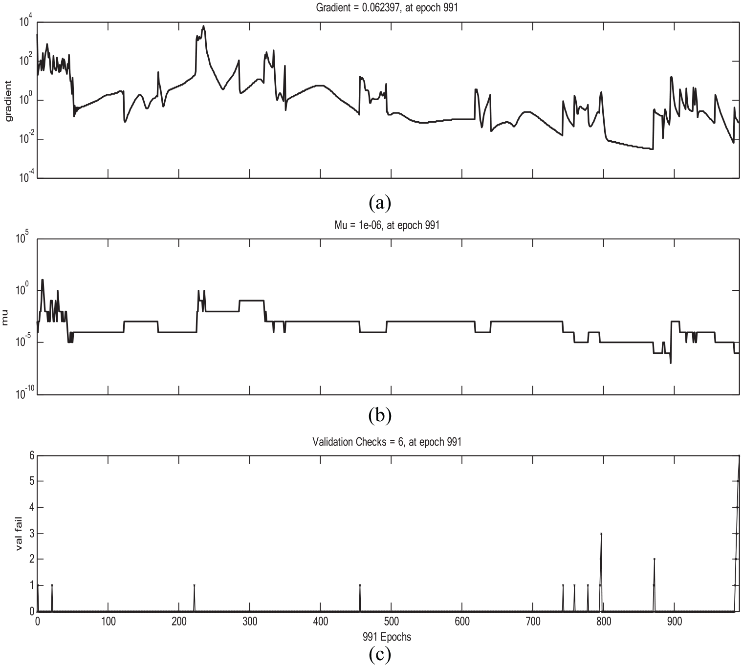
Graphs of the training quality with the testing set formed randomly: (a) The plots of the gradient (Gradient), adaptation
Figure 16 shows the learning, validation, testing, and progression of the best network performance. In this graph, Epoch refers to the iteration of the train network. A period is indicated as x-axis and a mean squared error (MSE) as y-axis. The best validation performance is reached at the 985th iteration.

Graph of network performance.
Geometric defects analysis of hip prosthesis
The hip prosthesis (Figure 17) is then measured using an optical probe (Figure 5(a) and (b)). After positioning the points cloud that are measured with regard to the nominal model of THA prostheses (Figure 18), the deviation errors between both models are evaluated. 7
Measured specimen.

Points cloud measured by the optical probe machine of prosthesis.
In this case, the points cloud is shown in Figure 18 such that the number of probed points n = 5404 of prosthesis N° 5 (Figure 17) after filtering. The shape defect is then estimated using the CAD software by measuring the distance between the points moved by the intelligence system and the surface of the nominal THA model.
Figure 19(a) illustrates the femoral stem of the hip prosthesis in 3D, by calculating the deviation errors E, we found that the error varies between Emax = +0.48101 mm and Emin = −0.13154 mm as it is visualized by the color degradation from red to violet. Figure 19(b) shows the left view of the femoral stem model of the PTH. It can be noted that the maximum value of deviation is on the head of the prosthesis however, the medium has less deviation. This comes down to the complexity of the head shape.

Deviation analysis between the model and the measured surface of the prosthesis: (a) Perspective projection of the hip prosthesis in three dimensions, (b) left view of hip prosthesis, (c) rear view of hip prosthesis and (d) right view of hip prosthesis.
Figure 19(a) illustrates the femoral stem of the hip prosthesis in 3D, by calculating the deviation errors E, we found that the error varies between Emax = +0.48101 mm and Emin = −0.13154 mm as it is visualized by the color degradation from red to purple.
Figure 19(b) shows the left view of the femoral stem model of THA. It can be noted that the maximum value of deviation is on the head of the prosthesis however, the medium has less deviation. This comes down to the complexity of the head shape.
Figure 19(c) shows the rear view of the femoral stem. It is found that the maximum value of deviation is focused at the end of the hip prosthesis due to the complexity of the head shape.
Figure 19(d) is the left view of the femoral stem model of THA. It can be seen that the maximum value of deviation is focused on the head of the femoral stem for the same reason as above.
The analysis results obtained show that the use of the neural network and the tools available in the CAD environment make it possible to estimate the shape defect of the manufactured THA.
The exploitation of the recalibrated points cloud can allow us to program finishing manufacturing operations to obtain prosthesis with the expected quality.
According to the Figure 20, we see that the difference between the real and the ideal model varies from −0.13154 to 0.48191 mm (tolerance interval = 0.2 mm while passing by a median value equal to 0.3 mm.

Topography of real and substitution surface of prosthesis (prosthesis section c-c (Figure 19(a)).
The surface considered must be between two left surfaces distant 0.2 mm, the two surfaces tangent to the measured surface and distant 0.1 mm.
The interval including negative values corresponds to hollows; on the other hand, the interval corresponding to positive values represents the peaks (Figure 19).
These errors are mainly caused by a calculating method of device drift during the active surfaces correction phase of the studied prosthesis. A bad influence is often an insufficient process-capability as well as excessive quality specifications, both resulting in high costs.
Effect of the specimen positions on the deviation
In this test part, the comparison is made according to the measurement positions of the specimen.
The first test
The specimen to be measured is in parallel with the reference according to Oxy plane but it is distanced l = 20

Comparison of the tolerance deviation according to the different positions: (a) Distanced l = 20 mm (angle of rotation relative to the reference αz = 0°), (b) distanced l = 40 mm, turned αz = 0°, (c) distanced l = 0 mm, turned αz = 30° and (d) distanced l = 0 mm, turned αz = 60° .
The second test
The specimen to be measured is distanced l = 40 mm, turned αz = 0° (not parallel to the reference according to Oxy plane) (Figure 21(b)).
The third test
The specimen to be measured is distanced l = 0 mm, turned αz = 30° (not parallel to the reference according to Oxy plane) (Figure 21(c)).
The fourth test
The specimen to be measured is distanced l = 0
The results obtained according to the different positions of the mesures specimen are shown in Figure 22. It can be seen that the deviation increases in the case of rotation and the opposite is true if only the deviation is small. Such that the mean of deviation is 0.009 mm in the translation and 0.85 in the rotations. According to the tests, it is observed that application of neuron network method on control of the validity of the specimen is influenced by the positions of the measured specimen.

The results obtained according to the different positions of the mesures specimen.
Conclusion
This paper presents a method for calculating shape defects of a free form surface. The work is applied to hip prostheses using the artificial intelligence, system using the points cloud as input and determining the position of the measurement points with respect to the CAD coordinate system. The proposed method makes it possible to visualize the shape defect without using a complex mathematical equations system. The first test is performed on a surface of the femoral stem. We found that this method gives good results in comparison of other existing methods. 2 The error of this method is in the neighborhood of micron scale, is neural network.
The measurement systems either by contact or without contact have advantages and disadvantages depending on the type of part to be measured (shape, material, etc.), the operations for taking measurements, deviation, visualization and system precision. The purpose of these measuring systems is to record the data necessary to define a left surface and to reconstruct it. We will have presented a method for removing thickness from deformed parts. The method will be tested on the hip prosthesis. This type of thin part was chosen because it has high deformability. The latter disrupts the final thickness of the prosthesis which is a functional characteristic after coinciding the model and the part made using neural network. Indeed, the quality of surface roughness is a greater constraint than the geometry of the parts produced.
Footnotes
Appendix
Notations

| Symbol | Designation |
|---|---|
| x 1r, y1r, z1r | Input to network (coordinate of points in the input) |
| x ie, yie, zie | Output of network (coordinate of points in the output) |
| ith | Neuron should be chosen to be a differentiable function |
| W | Weights of the network |
| w 0 | Weights |
| ∇E | Gradient |
| Error | |
| Total error | |
| Target output | |
| Output | |
| Activation function | |
| The weight from ith node j to the output neuron | |
| Input to network | |
| ωjk | Weights matrix |
| Learning rate | |
| Replacing by relationship | |
| jth | Output neuron |
Acknowledgements
We would like to thank the General Directorate of Scientific Research and Technological Development (DGRSDT) of Algeria and the Laboratory of Applied Biomechanics, Biomaterials (LABAB), ENP Oran, Algeria for their support in carrying out this research.
Handling Editor: Chenhui Liang
Declaration of conflicting interests
The author(s) declared no potential conflicts of interest with respect to the research, authorship, and/or publication of this article.
Funding
The author(s) received no financial support for the research, authorship, and/or publication of this article.