Fluid-structure interactions of internal pressure pipeline using the hierarchical finite element method

Abstract

We study the influence of the fluid with the structure in vibration between fluid and structure of a cylinder of circular section granted by the phenomenon of the interaction fluid structure of a conditioned flow of laminar nature and incompressible in the form of the macrostructure. These two phenomena by the mechanical relations of stresses according to displacements, modelled by a cylinder. The analysis of the vibrations of cylinders filled with fluid is studied with limiting conditions of fluid and the solid with the coupling conditioned by its limits of action-reaction in forces. The problem of the cylindrical pipe is formulated by deriving the deformation and the kinetic energies of the vibrating cylinder with and its fluid to have different natural frequencies, we use the principle of Hamilton change the problem in the expression of the equation cylindrical differential which gives three displacement functions in a system of partial differential equations of the cylindrical coordinate of circular section which meet the limiting conditions imposed at both ends. Let us apply the Navier-Stocks equation in cylindrical coordinates, with the fluid continuity equation, for the solid equation of mechanical behaviour of stresses in terms of displacement by strain. To obtain the results of natural frequencies we use the Galerkin method for solid and for Galerkin-time fluid. Where the liquid influences the inner surface of the circular cylinder, depending on the condition of the coupling that the stresses of the solid are equal to the stresses fluid. The modelling is done by a computer language (MATLAB), the hierarchical finite element method is presented by a Legendre polynomial with double integral of Rodrigues, to arrive at the final formula of the mass-rigidity matrix, which dissects on three parts (fluid, coupling and structure). Based on a comparison with experimental results. We continue to study some geometrical and physical parameters which influence the natural frequencies, in a proportional or inversely proportional way.

Introduction

The fluid-structure interaction is concerned with the behaviour of the mechanical system of the fluid and the solid at the same time of reactions of force or energy applied one on the other and verse versa where the flow is done around or inside the structure. Our study is based on the hierarchical finite element method as a new method of numerical resolution where we apply the function of the polynomial form (a form of the polynomial legend), on the stems of the quadratic finite element for the two systems to be studied. This is called version-h instead of version-p which takes up a lot of memory storage space, for long time convergence. Also, we use the polynomial of the velocity contributing to the displacements of the non-turbulent, irrotational laminar flow fluid (perfect flow).

Consider a closed space where the fluid circulates freely inside the cylinder of circular geometry at the entrance and the exit, it exerts the internal forces on the wall of the structure. As the internal flow of the secular section, we use the equation of Navier-stocks with cylindrical coordinates conditioned by perfect fluid. In all this, the resolution and algebraic form by the Eulerian approach consists in knowing the speed of the particles over time, by its spatial coordinates independent of time with dynamic fluid or the uniform flow, by applying the Lagrange method-temporary.

Concerning the structure, it is a body of deformable cylindrical geometrical shape, follows the physical properties according to the conditions of the material or to model it in cylindrical coordinates by the Lagrangian analytical approach and to solve this problem by transforming it of the relations constraints and displacement. One then applies the coupling between fluid and structure, which manifests systematically by stiffnesses of interface like forces formulated in stresses compared to displacements that are to say that the stresses of solid are equal to stresses of the fluid according to the matrix coupling penalty. We are developing a programme under Matlab, validated by several studied examples. The study of these examples made it possible to determine the influence of the physical and geometrical parameters on the Eigen frequencies of the coupled structure.

Some researchers have used different methods such as the deformable mesh and the finite volume of fluid methods to model the flows between fluid-structure or fluid-air, the majority of the works published in the field of interaction fluid structure its basis on the application of the finite element method, as references for solving differential equations in simulation and by different possible approach, it is methods take a lot of convergence time according to the precision ask for self-calculating by refining or the stability of simulation may, on the other hand, the hierarchical finite element method (HFEM) does not contain a refining tale nor long convergence time it is economical from the point of view of storage (minimisation of finite element) and computation (minimisation of the stiffness and mass matrices), which depends on shape function used on finite element rods, also a simple algorithm. We will cite some research works on the simulation and numerical modelling of the fluid-structure interaction domain, by the finite element method and the analytical method, except that the article^3,5,6 presents the hierarchical method, which does have not been used by most researchers on the effects of fluid-solid interaction, except for this work where it includes the method with penalty coupling such as Li and He ¹ have developed a numerical algorithm for a gas-melt two-phase flow using, the algebraic sub-grid scales-variational multi-scale (ASGS-VMS) finite element method. Montlaur et al. ² interior penalty method and a compact discontinuous Galerkin method are proposed and compared for the solution of the steady incompressible Navier–Stokes equations. Both compact formulations can be easily applied using high order piecewise divergence free approximations, leading to two uncoupled problems: one associated with velocity and hybrid pressure, and the other one only concerned with the computation of pressures in the elements interior. Numerical examples compare the efficiency and the accuracy of both proposed methods. Ouissi and Houmat ³ used bi-hierarchical finite elements for the analysis of the free vibration of non-axisymmetric shells of revolution to determine the parameters of frequency, on structures of different geometries. Houmat ⁴ used functions of arbitrary trigonometric shapes on a quadrilateral element to solve the problem of the different modes and the different degrees of freedom, which gives a decrease of the modes for an increase of the degrees of freedom.

In his article, Houmat ⁵ used hierarchical functions for the free three-dimensional vibratory analysis of a finite element according to the Legendre form of the orthogonal polynomial. Houmat ⁶ studied cylindrical shell vibrations using the wave propagation approach, with different boundary conditions and different geometrical conditions depending on the modal shapes. Buchanan and Yii ⁷ studied the influence of the boundary condition on the symmetrical vibration of the thick hollow cylinder. They used the finite element method with cylindrical coordinates of three dimensions. The resolution of the problem by the Rayleigh-Ritz method, with different boundary conditions to find the parameters of frequencies. Guo et al. ⁸ use the analysis of rotational vibrations of cylindrical shells by the finite element method for nonlinear geometry with strong deformation, determined the Eigen frequencies of the different modes by taking geometrical parameters constant. Zhang et al. ⁹ worked on the vibratory characteristics by the finite element method of a cylindrical shell carrying fluid by nonlinear displacement applying cylindrical coordinates, based on the principle of virtual work for solid and fluid. The work of Hamadi et al. ¹⁰ focuses on the development of a programme in MATLAB for modelling axisymmetric shells. Using the theory of Kirchhoff Love, and the elements CAXI_K and CAXI_L with curvilinear displacements of approximate linear form. The works of Bing-ru et al. ¹¹ based on analysis of calculi of different modes applying Donnell’s theory. The discretisation of the structure is done by the method of the finite elements where the length of the element is equal to the height of the cylinder. They used the wave propagation method with different boundary conditions to compute the frequency parameters and the circumferential and longitudinal modes. Seo et al. ¹² determine the response frequencies of cylindrical shells carrying a fluid, under internal pressure, using the finite element method for different boundary conditions using the principle of virtual work. They also determine natural frequencies by solving the equation of motion where the internal pressure is considered to be a uniform linear function with respect to displacement/force, related to circumferential and axial modes.

There are some new works like Hussain et al. ¹³ uses the FG method, based on Functionally Graded Materials (FGM). It is clearly that our work is based on isotropic material of a cylindrical of circular section and not materials with functional gradient (Functionally Graded Materials: FGM), or law of exponential volume fraction, because the goal of our work is applied the method of hierarchical finite elements in vibratory analysis for the natural frequencies, their close to real and their efficiency apart from the results obtained from this method, by different physical and geometric parameters in macro-structure according to the limit conditions to be controlled, several parameters intervene variable to choose well. Due to the variation in Young’s modulus, the neutral axis is not in the middle of the section as with isotropic structures, but it moves from the midplane. To determine the position of the neutral axis, we construct a new cylindrical coordinate system of the pipe, so that it has a new z axis. It is a new class of composite materials whose microstructure and composition vary gradually and continuously, because the study of this article on macrostructure with the optimal position in the mechanical performance of the structure has the presence of the fluid, instead of micro-structure, like work of Taj et al. ¹⁴ Like the work of Asghar et al. ¹⁵ and Abdel Wahid Tunisia, their study is based on small scale with the geometric influence of the proposed structure, by vibrational properties of double-walled carbon nanotubes. Chiral and zigzag rooted in Donnell’s shell model and non-local Eringen equations, with the numerical solution based on Donnell’s shell model for different natural frequency responses of DWCNTs. Or Hussain et al. ¹⁶ it is a continuation of Asghar’s work on a new method applied to the theory of the sander on SWCNT nanotubes by the Rayleigh-Ritz method of different limit condition at the end of the structure, according to the chair, zigzag and chiral with natural frequency variation, presented by several parameter, which is based on SWCNT length and thickness/radius, height/radius ratios, of NTC, by MATLAB in numerical resolution presented graphically. In these earlier literatures, we find that most of the work uses the classical finite element method(p-version). Which takes into account the equation of stability, which takes a lot of time to solve the problem, according to the required precision, but on the other hand the hierarchical finite element method, does not take into account the chosen precision of the refining to be studied with a short convergence time.

Our study is based on the application of the hierarchical finite element method for the cylindrical structure under pressure of the internal fluid with orthogonal Legendre polynomial in the vibrational analysis, of n degree of freedom by the finite element which and quadratic has four nodes and four stems, which replaces refinement or precision in finite elements by hierarchical finite elements. We are between two physical entities, solid and fluid that influence each other and vice versa with several methods of coupling between fluid and solid. It is for this reason the most common and the most reliable method for solving numerical analysis problems is the coupling by penalty, it is the interface between fluid and solid.

This HFEM method proves that the numerical values or simulation close to the experimental that the FEM method, or the percentage of the errors of different modes of vibration in Tables 1 and 2, allows to say that the results obtained apply to the reality of the experimental vibration analysis of the cylinder. As a simulation method which combines two mathematical entity finite element method and form-function; method proves that the numerical values or simulation close to the experimental that the FEM method, or the percentage of the errors of different modes of vibration in Tables 1 and 2, allows to say that the results obtained apply to the reality of the experimental vibration analysis of the cylinder.

Table 1.

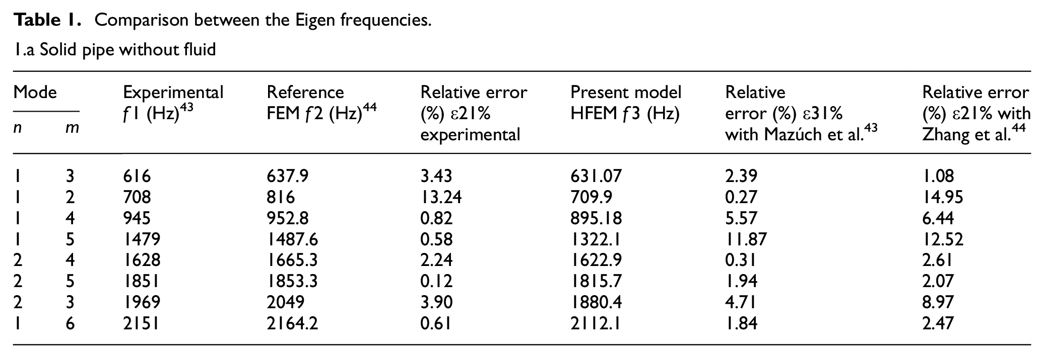
Comparison between the Eigen frequencies.

1.a Solid pipe without fluid

Mode		Experimentalf1 (Hz) 43	ReferenceFEM f2 (Hz) 44	Relative error(%) ε21%experimental	Present modelHFEM f3 (Hz)	Relativeerror (%) ε31%with Mazúch et al. 43	Relative error(%) ε21% withZhang et al. 44
n	m
1	3	616	637.9	3.43	631.07	2.39	1.08
1	2	708	816	13.24	709.9	0.27	14.95
1	4	945	952.8	0.82	895.18	5.57	6.44
1	5	1479	1487.6	0.58	1322.1	11.87	12.52
2	4	1628	1665.3	2.24	1622.9	0.31	2.61
2	5	1851	1853.3	0.12	1815.7	1.94	2.07
2	3	1969	2049	3.90	1880.4	4.71	8.97
1	6	2151	2164.2	0.61	2112.1	1.84	2.47

1.b Solid pipe with fluid

Mode		Experimentalf1 (Hz) 43	ReferenceFEM f2 (Hz) 44	Relative error (%)ε21% experimental	Present modelHFEM f3 (Hz)	Relative error(%) ε31% with Mazúch et al. 43	Relative error (%)ε21% withZhang et al. 44
n	m
1	3	388	370.1	4.84	385.76	0.58	4.06
1	2	421	431.2	2.37	433	2.77	0.42
1	4	628	597.2	5.16	630.02	0.32	5.21
1	5	1027	990.1	3.73	1022.2	0.47	3.14
2	4	1094	1046	4.59	1093.69	0.03	4.36
2	5	1245	1193.6	4.31	1257.5	0.99	5.08
2	3	1299	1234.7	5.21	1256.3	3.40	1.72
1	6	1546	1511.5	2.28	1567.4	1.37	3.57
2	6	1748	1676.2	4.28	1713.1	2.04	2.15

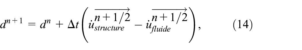
The phenomenon of vibration, indicates that the longitudinal (axial) vibration effects on the structure with the presence of the fluid, but in the circumferential vibration does not affect much on the structure, also the presence of the fluid inside the cylinder gives frequency stability, which means the partial absorption of vibratory shock waves.

Theory of structures

In all pipelines the fluid is transported inside the structure by pressure and velocity of the liquid all the way. By taking a hollow cylinder with a longitudinal axis z and inner radius r1 and outside r2 subjected to a pressure P1 on the inner surface, where displacements, deformations and stresses are determined according to the main vector directions (r, θ, z) of a cylindrical shell in revolution (Figure 1).

Figure 1.

Revolution cylindrical shell subjected to internal pressure.

The relation between displacements and deformation is given by Zienkiewicz and Taylor ¹⁷ :

$$\left\{\epsilon \right\}=\left[d\right]\left\{U\right\},$$

(1)

$$\left\{\epsilon \left(\mathrm{M}\right)\right\}=\left[\begin{array}{c}\begin{array}{c}\begin{array}{ccc}\frac{\partial }{\partial \mathrm{r}}\hfill & 0\hfill & 0\hfill \end{array}\hfill \\ \multicolumn{1}{c}{\begin{array}{ccc}\frac{1}{\mathrm{r}}\hfill & \frac{1}{\mathrm{r}}\frac{\partial }{\partial \theta }\hfill & 0\hfill \end{array}}\\ \multicolumn{1}{c}{\begin{array}{ccc}0\hfill & 0\hfill & \frac{\partial }{\partial \mathrm{z}}\hfill \end{array}}\end{array}\hfill \\ \multicolumn{1}{c}{\begin{array}{c}\begin{array}{ccc}\frac{1}{\mathrm{r}}\frac{\partial }{\partial \theta }\hfill & \frac{\partial }{\partial \theta }-\frac{1}{\mathrm{r}}\hfill & 0\hfill \end{array}\hfill \\ \multicolumn{1}{c}{\begin{array}{ccc}\frac{\partial }{\partial \mathrm{z}}\hfill & 0\hfill & \frac{\partial }{\partial \mathrm{r}}\hfill \end{array}}\\ \multicolumn{1}{c}{\begin{array}{ccc}0\hfill & \frac{\partial }{\partial \mathrm{z}}\hfill & \frac{1}{\mathrm{r}}\frac{\partial }{\partial \theta }\hfill \end{array}}\end{array}}\end{array}\right]\left\{\begin{array}{c}{\mathrm{u}}_{\mathrm{r}}\hfill \\ \multicolumn{1}{c}{{\mathrm{u}}_{\theta }}\\ \multicolumn{1}{c}{{\mathrm{u}}_{\mathrm{z}}}\end{array}\right\},$$

(2)

With $\left\{\begin{array}{c}{u}_r\hfill \\ \multicolumn{1}{c}{u_{\theta }}\\ \multicolumn{1}{c}{u_z}\end{array}\right\}=\left\{\begin{array}{c}v\hfill \\ \multicolumn{1}{c}{w}\\ \multicolumn{1}{c}{u}\end{array}\right\}$ , the displacement of the structure:

$$\left[d\right]=\left[\begin{array}{c}\begin{array}{c}\begin{array}{ccc}\frac{\partial }{\partial r}\hfill & 0\hfill & 0\hfill \end{array}\hfill \\ \multicolumn{1}{c}{\begin{array}{ccc}\frac{1}{r}\hfill & \frac{1}{r}\frac{\partial }{\partial \theta }\hfill & 0\hfill \end{array}}\\ \multicolumn{1}{c}{\begin{array}{ccc}0\hfill & 0\hfill & \frac{\partial }{\partial z}\hfill \end{array}}\end{array}\hfill \\ \multicolumn{1}{c}{\begin{array}{c}\begin{array}{ccc}\frac{1}{r}\frac{\partial }{\partial \theta }\hfill & \frac{\partial }{\partial \theta }-\frac{1}{r}\hfill & 0\hfill \end{array}\hfill \\ \multicolumn{1}{c}{\begin{array}{ccc}\frac{\partial }{\partial z}\hfill & 0\hfill & \frac{\partial }{\partial r}\hfill \end{array}}\\ \multicolumn{1}{c}{\begin{array}{ccc}0\hfill & \frac{\partial }{\partial z}\hfill & \frac{1}{r}\frac{\partial }{\partial \theta }\hfill \end{array}}\end{array}}\end{array}\right],$$

(3)

Using Hooke’s Law,

We obtain:

$$\begin{array}{c}\multicolumn{1}{c}{\left\{{\sigma }_s\left(M\right)\right\}=\frac{E}{(1+\upsilon )(1-2\upsilon )}}\\ \multicolumn{1}{c}{\left\{\begin{array}{c}\begin{array}{c}(1-\upsilon )\frac{\partial u_r}{\partial r}+\upsilon \frac{\partial u_z}{\partial z}+\upsilon \frac{1}{r}(u_r+\frac{\partial u_{\theta }}{\partial \theta })\hfill \\ \multicolumn{1}{c}{\upsilon \frac{u_r}{r}+(1-\upsilon )\frac{1}{r}(u_r+\frac{\partial u_{\theta }}{\partial \theta })+\upsilon \frac{\partial u_z}{\partial z}}\\ \multicolumn{1}{c}{\upsilon \frac{\partial u_z}{\partial z}+\upsilon \frac{1}{r}(u_r+\frac{\partial u_{\theta }}{\partial \theta })+(1-\upsilon )\frac{\partial u_z}{\partial z}}\end{array}\hfill \\ \multicolumn{1}{c}{\begin{array}{c}\frac{1-2\upsilon }{2}(\frac{\partial u_{\theta }}{\partial \theta }-\frac{u_{\theta }}{r}+\frac{1}{r}\frac{\partial u_r}{\partial \theta })\hfill \\ \multicolumn{1}{c}{\frac{1-2\upsilon }{2}(\frac{\partial u_r}{\partial z}+\frac{\partial u_z}{\partial r})}\\ \multicolumn{1}{c}{\frac{1-2\upsilon }{2}(\frac{1}{r}\frac{\partial u_z}{\partial \theta }+\frac{\partial u_{\theta }}{\partial z})}\end{array}}\end{array}\right\},}\end{array}$$

(4)

The relationship gives us the relation between the constraints of a point in accordance with displacements.

Theory of fluid

Applying the principle of conservation of motion amount, with and $\overrightarrow{\mathrm{t}}\left(\mathrm{n}\right)$ : constraint vector acting on one surface element dA and n: normal exterior. Projecting the equation on a coordinate system, we obtain Candel ¹⁸ and Tasos et al. ¹⁹ :

$$\frac{d}{\mathrm{dt}}{\int }_{V_{m\left(t\right)}}\rho v_i\mathrm{dV}={\int }_{V_m\left(t\right)}\rho g_i\mathrm{dV}+{\int }_{A_{m\left(t\right)}}{t}_i\left(n\right)\mathrm{dA},$$

(5)

or: $t_i\left(n\right)=T_{\mathrm{ij}}{n}_j$ and $T_{\mathrm{ji}}=T_{\mathrm{ij}}$

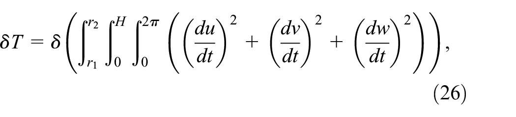
The terms of the three components of the stress vector are of the following form:

$$\begin{array}{c}{t}_1\left(n\right)=T_{11}{n}_1+T_{12}{n}_2+T_{13}{n}_3\hfill \\ \multicolumn{1}{c}{t_2\left(n\right)=T_{21}{n}_1+T_{22}{n}_2+T_{23}{n}_3}\\ \multicolumn{1}{c}{t_3\left(n\right)=T_{31}{n}_1+T_{32}{n}_2+T_{33}{n}_3}\end{array},$$

(6)

Knowing that from the physical stand point, the stress t is composed of two parts:

• The stress associated with pressure

• The stress associated with viscous forces

$$T_{\mathrm{ij}}=-p{\delta }_{\mathrm{ij}}+{\tau }_{\mathrm{ij}},$$

(7)

The equation (7) takes the form:

$$\frac{d}{\mathrm{dt}}{\int }_{V_{m\left(t\right)}}\rho v_i\mathrm{dV}={\int }_{V_m\left(t\right)}\rho g_i\mathrm{dV}+{\int }_{A_{m\left(t\right)}}(-p{\delta }_{\mathrm{ij}}+{\tau }_{\mathrm{ij}})n_j\mathrm{dA},$$

(8)

We use the Green-Ostrogradsky and Reynolds theorems respectively in equation (8). The integral on the domain in cylindrical coordinates (r, θ, z) gives the Navier-Stokes equation ²⁰ of irreversible incompressible ²¹ fluid, we obtain:

$$\begin{array}{c}\multicolumn{1}{c}{\rho \left[\frac{\partial {\stackrel{·}{u}}_r}{\partial t}\right]=\rho g_r-\frac{\partial p_r}{\partial r}+\mu [\frac{{\partial }^2{\stackrel{·}{u}}_r}{\partial r^2}+\frac{1}{r}\frac{{\partial }^2{\stackrel{·}{u}}_{\theta }}{\partial {\theta }^2}+\frac{1}{r^2}\frac{{\partial }^2{\stackrel{·}{u}}_r}{\partial {\theta }^2}+\frac{{\partial }^2{\stackrel{·}{u}}_r}{\partial z^2}-\frac{{\stackrel{·}{u}}_r}{r^2}-\frac{2}{r^2}\frac{\partial {\stackrel{·}{u}}_{\theta }}{\partial \theta }]}\\ \multicolumn{1}{c}{\rho \left[\frac{\partial {\stackrel{·}{u}}_{\theta }}{\partial t}\right]=\rho g_{\theta }-\frac{1}{r}\frac{\partial p_{\theta }}{\partial \theta }+\mu [\frac{{\partial }^2{\stackrel{·}{u}}_{\theta }}{\partial r^2}+\frac{1}{r}\frac{\partial {\stackrel{·}{u}}_{\theta }}{\partial r}+\frac{1}{r^2}\frac{{\partial }^2{\stackrel{·}{u}}_{\theta }}{\partial {\theta }^2}+\frac{{\partial }^2{\stackrel{·}{u}}_{\theta }}{\partial z^2}-\frac{{\stackrel{·}{u}}_{\theta }}{r^2}-\frac{2}{r^2}\frac{\partial {\stackrel{·}{u}}_r}{\partial \theta }]}\\ \multicolumn{1}{c}{\rho \left[\frac{\partial {\stackrel{·}{u}}_z}{\partial t}\right]=\rho g_z-\frac{\partial p_z}{\partial z}+\mu [\frac{{\partial }^2{\stackrel{·}{u}}_z}{\partial r^2}+\frac{1}{r}\frac{\partial {\stackrel{·}{u}}_z}{\partial r}+\frac{1}{r^2}\frac{{\partial }^2{\stackrel{·}{u}}_z}{\partial {\theta }^2}+\frac{{\partial }^2{\stackrel{·}{u}}_z}{\partial z^2}]}\end{array}\},$$

(9)

Boundary condition:

The flow in a pipe of circular section by laminar fluid, incompressible with circular section R, on a languor L, its gravity null by report the directions (z, θ).

$$\mathrm{or}{g}_{\theta }=0;g_z=0$$

with the uniform pressure gradient along the flow:

$$\frac{\partial p_r}{\partial r}=p;\frac{1}{r}\frac{\partial p_{\theta }}{\partial \theta }=p;\frac{\partial p_z}{\partial z}=p$$

at axial speed:

$${\stackrel{·}{u}}_z=0\Rightarrow \mathrm{if}r=R\mathrm{and}{\stackrel{·}{u}}_z=\stackrel{·}{U}\Rightarrow \mathrm{if}r=0,$$

where the fluid follows a function of form:

$$\stackrel{.}{u_z}\left(r\right)=\stackrel{.}{U}\left(1-{\left(r/R\right)}^2\right)$$

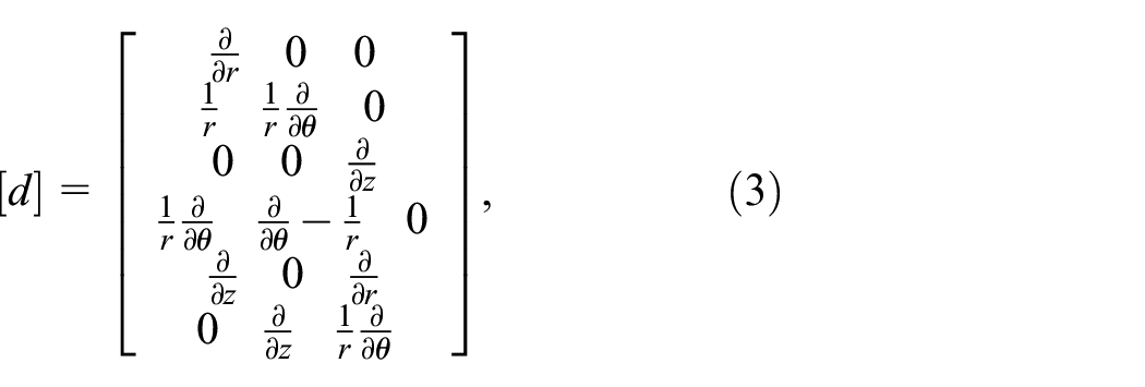
The constraint matrix of the solid point M in cylindrical coordinates (r, θ, z) is given by:

$$\left\{{\sigma }_f\left(M\right)\right\}=2\mu \left\{\begin{array}{l}\begin{array}{l}\frac{\partial {\stackrel{.}{u}}_r}{\partial r}-\frac{p_r}{2\mu }+\frac{1}{2}\left(\frac{1}{r}\frac{\partial {\stackrel{.}{u}}_{\theta }}{\partial \theta }-\frac{{\stackrel{.}{u}}_{\theta }}{r}+\frac{1}{r}\frac{\partial {\stackrel{.}{u}}_r}{\partial \theta }\right)+\frac{1}{2}\left(\frac{\partial {\stackrel{.}{u}}_z}{\partial z}+\frac{\partial {\stackrel{.}{u}}_r}{\partial r}\right)\hfill \\ \frac{1}{2}\left(\frac{1}{r}\frac{\partial {\stackrel{.}{u}}_{\theta }}{\partial \theta }-\frac{{\stackrel{.}{u}}_{\theta }}{r}+\frac{1}{r}\frac{\partial {\stackrel{.}{u}}_r}{\partial \theta }\right)+\left(\frac{1}{r}\frac{\partial {\stackrel{.}{u}}_{\theta }}{\partial \theta }+\frac{{\stackrel{.}{u}}_r}{r}\right)-\frac{p_{\theta }}{2\mu }+\frac{1}{2}\left(\frac{1}{r}\frac{\partial {\stackrel{.}{u}}_z}{\partial \theta }+\frac{\partial {\stackrel{.}{u}}_{\theta }}{\partial z}\right)\hfill \end{array}\hfill \\ \begin{array}{l}\frac{1}{2}\left(\frac{\partial {\stackrel{.}{u}}_r}{\partial z}+\frac{\partial {\stackrel{.}{u}}_z}{\partial r}\right)+\frac{1}{2}\left(\frac{1}{r}\frac{\partial {\stackrel{.}{u}}_z}{\partial \theta }+\frac{\partial {\stackrel{.}{u}}_{\theta }}{\partial z}\right)+\frac{\partial {\stackrel{.}{u}}_z}{\partial z}-\frac{p_z}{2\mu }\hfill \\ \frac{1}{2}\left(\frac{1}{r}\frac{\partial {\stackrel{.}{u}}_{\theta }}{\partial \theta }-\frac{{\stackrel{.}{u}}_{\theta }}{r}+\frac{1}{r}\frac{\partial {\stackrel{.}{u}}_r}{\partial \theta }\right)\hfill \end{array}\hfill \\ \begin{array}{c}\frac{1}{2}\left(\frac{\partial {\stackrel{.}{u}}_r}{\partial z}+\frac{\partial {\stackrel{.}{u}}_z}{\partial r}\right)\\ \frac{1}{2}\left(\frac{1}{r}\frac{\partial {\stackrel{.}{u}}_z}{\partial \theta }+\frac{\partial {\stackrel{.}{u}}_{\theta }}{\partial z}\right)\end{array}\hfill \end{array}\right\},$$

(10)

Coupling theory by the penalty method

Method SPH

The Smoothed Particle Hydrodynamics (SPH) method, is characterised by the mass of the particles, two amounts of discretisation are the distance between the particles and the diameter of the particle. The principle is to approximate a field $\overrightarrow{\stackrel{·}{\mathrm{u}}}$ on a domain ω by a set of discretisation points called particles. In each of these particles, the integral formulation of the field can be written. In each of these particles integral formulation of the field can be written.

$$\overrightarrow{\stackrel{·}{u}}\left(\overrightarrow{X}\right)={\int }_w\overrightarrow{\stackrel{·}{u}}\left(\overrightarrow{Y}\right)\delta (\overrightarrow{X}-\overrightarrow{Y})\mathrm{dw},$$

(11)

If ${\rho }_j$ and $m_j$ respectively represent the density and mass of a particle j, the integral of equation (11) can be approximated by a Monte Carlo quadrature:

$$\overrightarrow{\stackrel{·}{u}}\left({\overrightarrow{X}}_i\right)=\sum _i\frac{m_j}{{\rho }_j}\overrightarrow{\stackrel{·}{u}}\left({\overrightarrow{X}}_j\right)W(\Vert {\overrightarrow{X}}_i-{\overrightarrow{X}}_j\Vert ,h),$$

(12)

The SPH/FEM coupling is based on a penalised contact method. Fluid particles are the slave ‘nodes’. The particle enters a structure element with a distance d (Figure 2) and the applied force is proportional to this distance: f = kd where k is the stiffness by penalisation.

Figure 2.

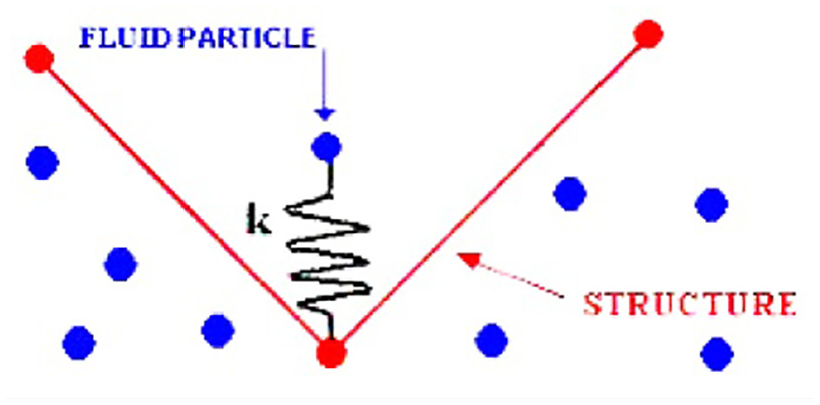
Coupling SPH/FEM.

Method SPH with FEM

This coupling is used to manage the fluid-structure interaction between a Lagrangian mesh for the structure, which follows an Eulerian mesh for the fluid. The Lagrangian mesh being immersed in the Eulerian grid. ²²

The most common SPH method in fluid mechanics uses Lagrangian, concerning Eulerian coordinates, a coherent first-order numerical method. To make the SPH method consistent, several methods have been proposed, for example, in Monaghan ²³ he assumed that. Finally, with the equation of motion for the fluid particle i, the semi-discrete equations for inviscid fluids are written as Li ²⁴ :

$$\{\begin{array}{c}\frac{d{x}_i}{\mathrm{dt}}=v_i\hfill \\ \multicolumn{1}{c}{\frac{d{\rho }_i}{\mathrm{dt}}={\rho }_i\sum _{j\in D_i}(v_j-v_i)·{\nabla }_i{W}_{\mathrm{ij}}{w}_j}\\ \multicolumn{1}{c}{\frac{d{v}_i}{\mathrm{dt}}=g_i-\sum _{j\in D_i}{m}_j(\frac{p_j}{{\rho }_j^2}+\frac{p_i}{{\rho }_i^2}+{\Pi }_{\mathrm{ij}}){\nabla }_j{W}_{\mathrm{ij}}}\end{array},$$

(13)

The study of convergence according to the order of the polynomial is represented in Figure 3. The fluid particle coupled to the internal point of the structure can be assimilated to a new node, physically connected to the other nodes, by the functions of Eulerian form and the coupling force exerted on the particle being distributed to the element nodes by the inverse of these same shape functions.

Figure 3.

Coupling SPH/FEM/FEM.

Relative displacement built starting from the Eulerian variables is given, by the time step in product relative speed, normal to the element of structure: $\mathrm{\Delta }\mathrm{t}({\stackrel{·}{\mathrm{u}}}_{\mathrm{structure}}^{\overrightarrow{\mathrm{n}+1/2}}-{\stackrel{·}{\mathrm{u}}}_{\mathrm{fluide}}^{\overrightarrow{\mathrm{n}+1/2}})$ .

The penetration at each cycle is up to date by:

$$d^{n+1}=d^n+\mathrm{\Delta }t({\stackrel{·}{u}}_{\mathrm{structure}}^{\overrightarrow{n+1/2}}-{\stackrel{·}{u}}_{\mathrm{fluide}}^{\overrightarrow{n+1/2}}),$$

(14)

If $d^{n+1}\overrightarrow{n^s}$ or $\overrightarrow{n^s}$ is the vector normal to the structure, the coupling algorithm is started. Once the penetration determined, as for the contact by penalisation, a restoring force, $F_{s\to f}$ is applied to the fluid particle, the reaction to this force being distributed to the structural nodes by the functions of nodal forms $N_I$ :

$$N_I{F_{s\to f}}^{n+1}=-N_{I}k{d}^{n+1},$$

(15)

Method FEM with FEM

The method of finish element method by finite element method (FEM/EFM) is characterised by the linking of the finite element structure to that of the fluid by the stiffness of the two nodes at the interface level. The slip is neglected^25,26 (Figure 4).

Figure 4.

Coupling FEM/FEM.

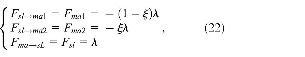
In order to present this method, we consider a two-dimensional case. There must be a master element with two nodes nodes ma1, ma2 and a slave node sl. In order to be able to control the master element, a conformal and normal repulsive force must be applied. The challenge then is to calculate the value of this force. Taking into account the local coordinate of the master element and by considering that the normal forces and applying the principle of action and reaction, we get:

$${\mathrm{F}}_{\mathrm{ma}\to \mathrm{sl}}=-{\mathrm{F}}_{\mathrm{sl}\to \mathrm{ma}}\mathrm{with}{\mathrm{F}}_{\mathrm{ma}\to \mathrm{sl}}={\mathrm{F}}_{\mathrm{ma}1\to \mathrm{sl}}+{\mathrm{F}}_{\mathrm{ma}2\to \mathrm{sl}},$$

(16)

Let us now involve weighting of the reaction force of the slave node on the nodes of the master element, through the variable ξ and defined by:

$$\xi =\frac{y_{\mathrm{sl}}-y_{\mathrm{ma}1}}{y_{\mathrm{ma}2}-y_{\mathrm{ma}1}},$$

(17)

We can, then, write the equations:

$$F_{\mathrm{ma}1\to \mathrm{sl}}=(1-\xi )F_{\mathrm{ma}\to \mathrm{sl}}\mathrm{and}{F}_{\mathrm{ma}2\to \mathrm{sl}}=\xi F_{\mathrm{ma}\to \mathrm{sl}},$$

(18)

In our case the coupling is stiff and without damping. The term ‘master’ and ‘slave’ are generally attributed to the fluid and the structure respectively. The stiffness of the spring is represented by k with the distances between slave and master by u_sa, u_ml which are represented respectively. Disposing, at the interface, fictitious springs in tension between all the penetrating nodes and the contact surface, the equilibrium position of these springs corresponding to a slave node positioned on the master segment.

$$F_{\mathrm{ma}->\mathrm{sl}}=-k(u_{\mathrm{sl}}-u_{\mathrm{ma}}),$$

(19)

Multiple method of Lagrange

The Lagrange multiplier method is more natural than the penalty method, at the expense of a higher calculation time. The general idea is to find, respecting the spatial constraint resulting from the positions of the slave and master nodes, the contact force verifying at best the equation of conservation of the quantity of movement. ²⁷

By introducing the locator function φ of the slave node in relation to the master element,

$$\varnothing =y_{\mathrm{sl}}-(1-\xi )y_{\mathrm{ma}1}+\xi y_{\mathrm{ma}2},$$

(20)

The forces $F_i$ interactions where $i\in \{\mathrm{sl},m{a}_1,m{a}_2\}$ applied to the node i can be written, involving a Lagrange multiplier λ having the dimension of a force:

$$F_i=\lambda \frac{\partial \varnothing }{\partial y_i},$$

(21)

We can, then, find the expression of the interaction forces introduced into the penalty method:

$$\{\begin{array}{c}{F}_{\mathrm{sl}\to \mathrm{ma}1}=F_{\mathrm{ma}1}=-(1-\xi )\lambda \hfill \\ \multicolumn{1}{c}{F_{\mathrm{sl}\to \mathrm{ma}2}=F_{\mathrm{ma}2}=-\xi \lambda }\\ \multicolumn{1}{c}{F_{\mathrm{ma}\to \mathrm{sL}}=F_{\mathrm{sl}}=\lambda }\end{array},$$

(22)

The determination of Lagrange multipliers is generally done with the iterative method which is costly in computation time than the Gauss-Seidel type method.^28,29

Formulation

The potential energy of a structure is determined by Philip ³⁰ :

$$\delta U_s=\frac{1}{2}\int {\left\{\delta {\epsilon }_s\right\}}^T\left\{{\sigma }_s\right\}\mathrm{dV},$$

(23)

The (23) expressions of a cylindrical shell in cylindrical coordinates take the following form:

$$\delta U_s=\frac{1}{2}{\int }_{r_1}^{r_2}{\int }_0^H{\int }_0^{2\pi }\left(\delta {\left\{\begin{array}{c}\begin{array}{c}{\epsilon }_{\mathrm{rr}}\hfill \\ \multicolumn{1}{c}{{\epsilon }_{\mathrm{zz}}}\\ \multicolumn{1}{c}{{\epsilon }_{\theta \theta }}\end{array}\hfill \\ \multicolumn{1}{c}{\begin{array}{c}{\gamma }_{\mathrm{rz}}\hfill \\ \multicolumn{1}{c}{{\gamma }_{r\theta }}\\ \multicolumn{1}{c}{{\gamma }_{z\theta }}\end{array}}\end{array}\right\}}^T\left[D\right]\left\{\begin{array}{c}\begin{array}{c}{\epsilon }_{\mathrm{rr}}\hfill \\ \multicolumn{1}{c}{{\epsilon }_{\mathrm{zz}}}\\ \multicolumn{1}{c}{{\epsilon }_{\theta \theta }}\end{array}\hfill \\ \multicolumn{1}{c}{\begin{array}{c}{\gamma }_{\mathrm{rz}}\hfill \\ \multicolumn{1}{c}{{\gamma }_{r\theta }}\\ \multicolumn{1}{c}{{\gamma }_{z\theta }}\end{array}}\end{array}\right\}\right)\mathrm{rdrdzd}\theta ,$$

(24)

For a solid to be in equilibrium, works of external forces should be equal to the kinetic energy ³¹ :

$$\delta T=\delta W,$$

(25)

Elementary potential energy is given by:

$$\delta T=\delta \left({\int }_{r_1}^{r_2}{\int }_0^H{\int }_0^{2\pi }({\left(\frac{\mathrm{du}}{\mathrm{dt}}\right)}^2+{\left(\frac{\mathrm{dv}}{\mathrm{dt}}\right)}^2+{\left(\frac{\mathrm{dw}}{\mathrm{dt}}\right)}^2)\right),$$

(26)

The penalty method belongs to regulation techniques on the method of contact between two different media. It takes into account the fact that the unilateral stresses or the normal forces of contact are proportional to displacement. The penalty method considers the normal component of the contact force as follows ³² :

$$f_n\left({\delta }_n,\stackrel{.}{{\delta }_n}\right)=\{\begin{array}{c}-k{\delta }_n-b{\stackrel{.}{\delta }}_{n}si{\delta }_n<0\\ 0si{\delta }_n\ge 0\end{array},$$

(27)

The value of the interference ${\mathrm{\delta }}_{\mathrm{n}}$ contact is measured by a constant distance that is homogeneous to a given volume. If it is negative, then there is the contact force, which is penalised by a coefficient k, the higher value, the closer you get to the Signorini contact law.

But from a mathematical point of view, the coefficient k must be falling towards infinity to obtain the most accurate approximation possible. In numerical modelling to avoid the problems of convergence in Figure 5.

Figure 5.

Law of Signorini (a) that can be corrected by a penalty factor k =  ${\mathbf{\alpha }}_{\mathbf{P}}$ (b).

This approach allows us to determine the equation of motion as follows:

$$\{\begin{array}{c}\multicolumn{1}{c}{m\left\{\stackrel{··}{\mathrm{u}}\right\}+k{\delta }_n=f\mathrm{si}{\delta }_n<0}\\ \multicolumn{1}{c}{m\left\{\stackrel{··}{\mathrm{u}}\right\}=f\mathrm{si}{\delta }_n\ge 0}\end{array},$$

(28)

The boundary conditions are defined by Woldemariam and Lemu ³³ :

• Boundary condition of the solid:

  $$-\left[{\sigma }_s\right]\left\{n\right\}+\left\{f_s\right\}=0\mathrm{in}{S}_s\iff \left[{\sigma }_s\right]\left\{n\right\}=\left\{f_s\right\},$$

  (29)

• Boundary condition of the fluid:

  $$-\left[{\sigma }_f\right]\left\{n\right\}+\left\{f_f\right\}=0\mathrm{in}{S}_f\iff \left[{\sigma }_f\right]\left\{n\right\}=\left\{f_f\right\},$$

  (30)

Since we have a fluid-structure interaction, the principle of action-reaction imposes equal amounts of both (29) and (30).

We have the boundary condition of interaction fluid-cylinder:

$$\left[{\sigma }_s\right]\left\{n\right\}=\left[{\sigma }_f\right]\left\{n\right\},$$

(31)

Where

$$\left\{f_s\right\}=\left\{f_f\right\},$$

(32)

The contact forces in case of penalty method are determined by Hui et al. ³⁴ :

$$\left\{f_s\right\}={\alpha }_P\left[g_s\right]\mathrm{and}\left\{f_f\right\}={\alpha }_P\left[g_f\right],$$

(33)

${\alpha }_P$ : Factor penalty.

The contact being the type strength, quantities $\left[{\mathrm{g}}_{\mathrm{s}}\right]$ and $\left[g_f\right]$ are determined by Mahmoud et al. ³⁵ :

$$\begin{array}{c}\left[g_s\right]=\left[\begin{array}{cc}k\hfill & -k\hfill \\ \multicolumn{1}{c}{-k}& k\hfill \end{array}\right]\left\{\begin{array}{c}{u}_{\mathrm{ir}}\hfill \\ \multicolumn{1}{c}{w_{\mathrm{iz}}}\end{array}\right\}\hfill \\ \multicolumn{1}{c}{\left[g_f\right]=\left[\begin{array}{cc}k\hfill & -k\hfill \\ \multicolumn{1}{c}{-k}& k\hfill \end{array}\right]\left\{\begin{array}{c}{u}_{\mathrm{ir}}\hfill \\ \multicolumn{1}{c}{w_{\mathrm{iz}}}\end{array}\right\}}\end{array},$$

(34)

where:

$$\left[g_{\mathrm{sf}}\right]=\left[\begin{array}{cc}\begin{array}{cc}k\hfill & 0\hfill \\ \multicolumn{1}{c}{0}& k\hfill \end{array}\hfill & \begin{array}{cc}-k\hfill & 0\hfill \\ \multicolumn{1}{c}{0}& -k\hfill \end{array}\hfill \\ \multicolumn{1}{c}{\begin{array}{cc}-k\hfill & 0\hfill \\ \multicolumn{1}{c}{0}& -k\hfill \end{array}}& \begin{array}{cc}k\hfill & 0\hfill \\ \multicolumn{1}{c}{0}& k\hfill \end{array}\hfill \end{array}\right]\left\{\begin{array}{c}\begin{array}{c}{u}_{\mathrm{ir}}\hfill \\ \multicolumn{1}{c}{w_{\mathrm{iz}}}\end{array}\hfill \\ \multicolumn{1}{c}{\begin{array}{c}{u}_{\mathrm{ir}}\hfill \\ \multicolumn{1}{c}{w_{\mathrm{iz}}}\end{array}}\end{array}\right\},$$

(35)

To comply with the convergence of contact penalty, ${\mathrm{g}}_{\mathrm{sf}}$ should be equal to ${{\mathrm{g}}_{\mathrm{sf}}}^2$ positively and ${\alpha }_{\mathrm{P}}$ should be framed between 10⁴ and 10⁹, so the form of (37) becomes:

$$\left[G\right]=\left[g_{\mathrm{sf}}\right]{\left[g_{\mathrm{sf}}\right]}^T={\left[g_{\mathrm{sf}}\right]}^2,$$

(36)

So, the fluid-structure stiffness takes the following form

$$\left[K_{\mathrm{SYS}}\right]=\left[K_{\mathrm{FS}}\right]+{\alpha }_P\left(\left[g_{\mathrm{sf}}\right]{\left[g_{\mathrm{sf}}\right]}^T\right)=\left[K_{\mathrm{FS}}\right]+{\alpha }_P\left[G\right],$$

(37)

Applying the principle of Hamilton. ³⁶

$${\int }_{t_1}^{t_2}(\delta T-\delta U)\mathrm{dt}=0,$$

(38)

We obtain the equation of motion structure.

$$({\left[\mathrm{M}\right]}_{\mathrm{s}}^{\mathrm{e}}\left\{\stackrel{··}{\mathrm{U}}\right\}+{\left[\mathrm{K}\right]}_{\mathrm{s}}^{\mathrm{e}}\left\{\mathrm{U}\right\}+{\left\{\mathrm{F}\right\}}_{\mathrm{s}}^{\mathrm{e}})=0,$$

(39)

The Navier-Stokes equation (9) contains strong variational terms, so the Galerkin principle is applied to weaken the formulation for numerical discretisation. ³⁷ The equation of motion of the fluid is equal to:

$$({\left[\mathrm{M}\right]}_{\mathrm{f}}^{\mathrm{e}}\left\{\stackrel{··}{\mathrm{U}}\right\}\mathrm{\Delta }t+{\left[\mathrm{K}\right]}_{\mathrm{f}}^{\mathrm{e}}\left\{\stackrel{·}{\mathrm{U}}\right\}\mathrm{\Delta }t+{\left\{\mathrm{F}\right\}}_{\mathrm{f}}^{\mathrm{e}})=0,$$

(40)

The equation of motion of the cylindrical shell is represented with respect to the radial, circumferential and axial displacement in the coordinate system (r, θ, z) boundary conditions.

The free vibration of the components u_r, u_èç and u_z are of the form.^38,39

$$\begin{array}{c}\multicolumn{1}{c}{u(r,\theta ,z,t)=u_r\cos \left(m\theta \right)\cos \left(\frac{n\pi z}{L}\right)\cos \mathrm{wt}}\\ \multicolumn{1}{c}{v(r,\theta ,z,t)=u_{\theta }\cos \left(m\theta \right)\cos \left(\frac{n\pi z}{L}\right)\cos \mathrm{wt}}\\ \multicolumn{1}{c}{w(r,\theta ,z,t)=u_z\sin \left(m\theta \right)\cos \left(\frac{n\pi z}{L}\right)\cos \mathrm{wt}}\end{array},$$

(41)

Where $u_r,u_{\theta },u_z$ are functions of displacements for nodal interpolation functions for quadratic finite element. The coefficient λ determined from the boundary conditions; for Simply supported a cylinder, λ=nπ R/L, for a cylinder whose ends are clamped λ = (n+0.3)π R/L où $u_r$ , $u_{\theta }$ , $u_z$ .

Methods of hierarchical finished elements

In the finite element method where the h-version requires refinement of the mesh to obtain a good precision, but the p-version, on the other hand, is to improve the precision of the numerical model of the structure by increasing the degree of freedom of function to use on the go. This is the principle of the hierarchical finite element method (H-FEM), where element segments are the variable functions.

The (h-FEM) has several advantages over the h-version:

1. It does not require a big change in the mesh for the accuracy of the solution.

2. The stiffness and mass matrices have the coating property, that is to say that the displacement functions f1 are always sub-matrices.

3. The embedding property can be used to prove that the Eigenvalues corresponding to the function (f1 + 1), of displacement frame the Eigenvalues corresponding to the functions of f1. This is called the principle of inclusion.

4. Simple structures can be modelled using a single element.

5. The elements of different start polynomials are not difficult. Therefore, it is possible to include additional degrees of freedom when needed.

6. The objective of the h-FEM is to give accurate results with fewer degrees of freedom of the p-version.

The most commonly used hierarchical functions are derived from Legendre polynomials ⁴⁰ namely:

$$f_m\left(\xi \right)=\frac{1}{m!{(-2)}^m}\frac{d^m}{d{\xi }^m}\left\{{(1-{\xi }^2)}^m\right\}-1\le \xi \le +1,$$

(42)

That satisfy the orthogonality relation ${\int }_{-1}^1{f}_i\left(\xi \right)f_j\left(\xi \right)d\xi =\frac{2}{2i+1}{\delta }_{\mathrm{ij}}$ .

where ${\delta }_{\mathrm{ij}}$ is the Kronecher delta function.

The orthogonality of the Legendre polynomial ⁴¹ in the interval [−1 1], is made by the integration (42) and that all their derivatives of lower order disappear at ξ = ±1, we obtain the following numerical formula ⁴² :

$$f_m^r\left(\xi \right)=\sum _{n=0}^{m/2}\frac{{(-1)}^n}{n!2^n}\frac{(2m-2n-2s-1)!!}{(m-2n)!}{\xi }^{m-2n},$$

(43)

With

!! m = m (m − 2) ⋯ (2ou1), 0!! = 1 (−1) = 1!!

Cylindrical shell vibrating by the HFEM

The axial displacement, u, is expressed as:

$$u=\sum _{n=0}^p{g}_r\left(\xi \right)q_r,$$

(44)

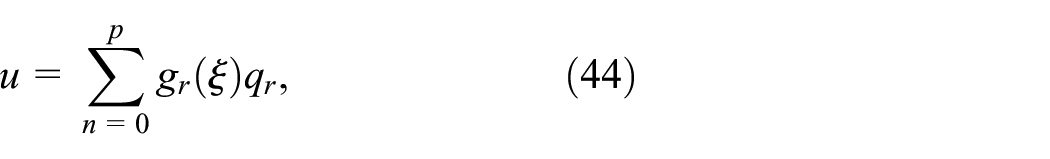
Where q is the number of degrees of the function associated with the interval −1 ≤ ξ ≤ 1, the hierarchical functions g_r (ξ), for r > 2, are for s = 1 and m = (r − 1) in l equation (42). This gives:

$$g_r\left(\xi \right)=\sum _{n=0}^{(r-1)/2}\frac{{(-1)}^n}{n!2^n}\frac{(2m-2n-5)!!}{(r-2n-1)!}{\xi }^{r-2n-1},$$

(45)

The lateral displacement, v, is expressed by Babuška et al. ⁴² :

$$v=\sum _{n=0}^p{f}_r\left(\xi \right)q_r,$$

(46)

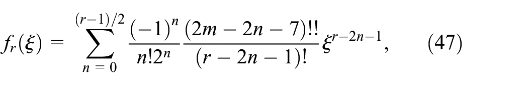
The hierarchical functions f_r (ξ), for $r>4$ , are obtained by putting $s=2$ and $m=(r-1)$ in equation (46). This gives:

$$f_r\left(\xi \right)=\sum _{n=0}^{(r-1)/2}\frac{{(-1)}^n}{n!2^n}\frac{(2m-2n-7)!!}{(r-2n-1)!}{\xi }^{r-2n-1},$$

(47)

The h-FEM can be used to calculate the vibration characteristics, the displacements of the points of a cylindrical shell or the tangential components $u_r,u_{\theta },u_z,$ of the normal component. The trips are given by:

$$|\begin{array}{c}{u}_r(\xi ,\eta )=\sum _{r=1}^q\sum _{s=1}^p{g}_s\left(\xi \right)g_s\left(\eta \right)U_{\mathrm{rs}}\hfill \\ \multicolumn{1}{c}{u_{\theta }(\xi ,\eta )=\sum _{r=1}^q\sum _{s=1}^p{g}_s\left(\xi \right)g_s\left(\eta \right)V_{\mathrm{rs}}}\\ \multicolumn{1}{c}{u_z(\xi ,\eta )=\sum _{r=1}^q\sum _{s=1}^p{g}_s\left(\xi \right)g_s\left(\eta \right)W_{\mathrm{rs}}}\end{array},$$

(48)

Validation of the structure

The validation of our programme is done by studying the convergence and the comparison of the determined results, with the results of other authors, according to the hierarchical finite element model which contains a solid and fluid finite element in Figure 6. With interface between the two, by the variable geometric size the element stems it is nothing but a polynomial of n degree of freedom, used as a grid, according to the convergence of the polynomial by The Gauss–Seidel method, also known as the Liebmann method, is an iterative method used to solve a system of linear equations shown in Figures 7 and 8.

Figure 6.

Fluid-structure interaction by penalty coupling.

Figure 7.

Convergence of the polynomial for different degrees of solid freedom.

Figure 8.

Convergence of the polynomial for different degrees of fluid freedom.

In the following tables, we compare the Eigen frequencies of a clamped-clamped pipe with different physical and mechanical characteristics with those of the experimental values, ⁴³ and the results of the reference ⁴⁴ with the geometric and physical conditions for solid pipe without fluid E = 2.05 × 10¹¹ N/m², ϑ = 0.3, R/h = 51.5, L/R = 2.99, ρ_s = 7800 kg/m³ and solid pipe with fluid E = 2.05 × 10¹¹ N/m², ϑ = 0.3, R/h = 51.5, L/R = 2.99, ρ_f/ρ_s = 0.128 and p₀ = 0 kPa.

We note that the results are close to experimental results and those of reference ⁴³ and we also notice the natural frequencies determined by finite element method are closer to experimental results than the reference. ⁴⁴ The percentages of errors $\epsilon {\mathrm{\%}}_{\mathrm{ij}}$ are defined in the tables by $\epsilon {\mathrm{\%}}_{\mathrm{ij}}=|(100(f_i-f_j)/f_i)|$ and Figure 9.

Figure 9.

Relative error $\epsilon \%$ of Table 1.

Case studies

We determine the frequency parameters of a cylindrical pipe by free-clamp condition by varying the parameters physical and geometrical following:

Variation of the thickness of the cylindrical

Taking the constant longitudinal mode, we determine the variation of the circumferential modes according to the thickness of the pipe we obtain the following graphin Figure 10.

Figure 10.

Variation of the thickness by parameter frequency relative to the variable modes circumferential solid.

Variation of the length of the cylindrical

Taking into consideration that the modes constant longitudinal vibration, one determines the variation of the circumferential modes according to the length of the cylinder one obtains the following graphin Figure 11.

Figure 11.

Variation of the length by parameter frequency relative to the circumferential variable modes solid.

Variation in the length of the pipe with and it’s fluid

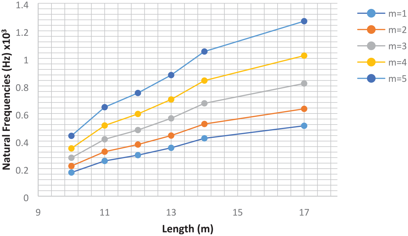
By taking the constant circumferential modes, one determines the variation of the longitudinal modes according to the thickness of the pipe one obtains the following graph in Figures 12 and 13.

Figure 12.

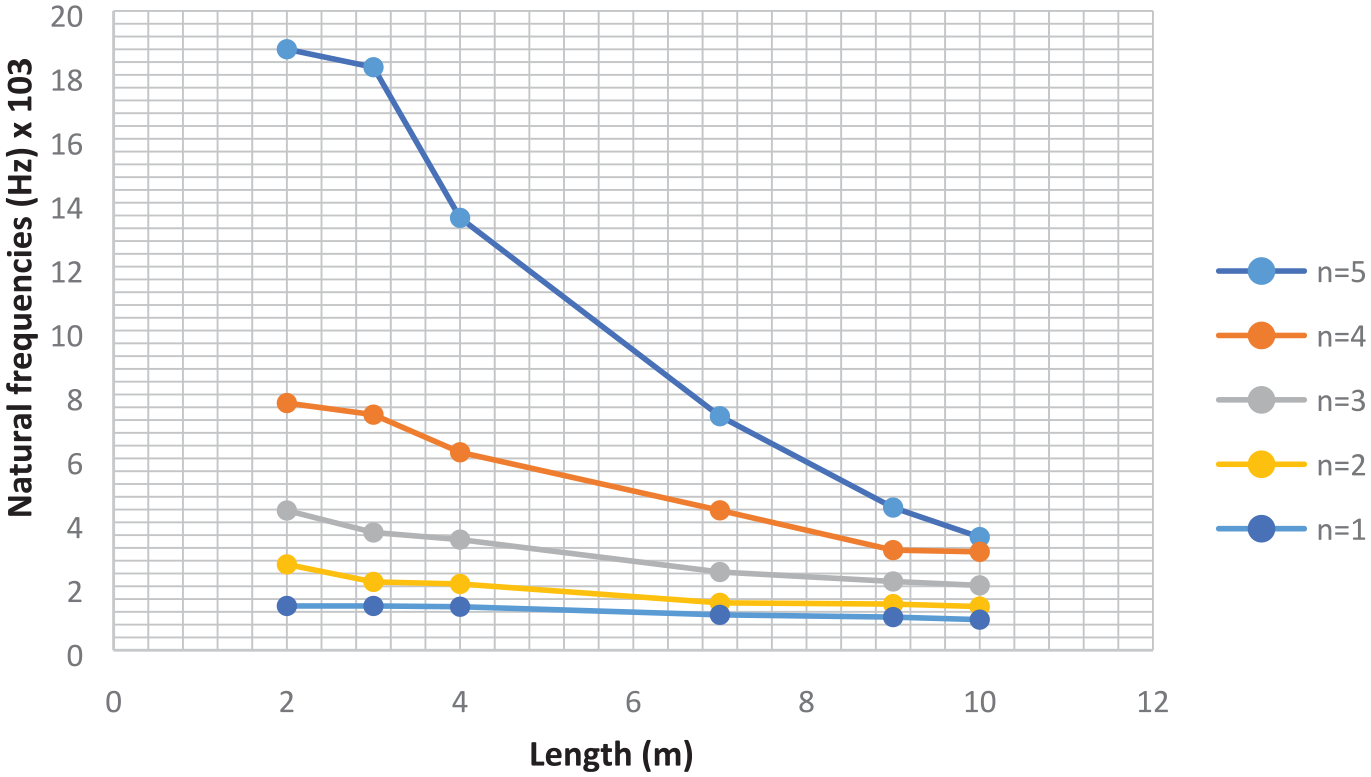
Variation of lengths relative by parameter frequency for variable longitudinal modes solid.

Figure 13.

Variation of lengths by parameter frequency for longitudinal modes variable solid with fluid.

Variation of the radius of the cylinder with fluid

By taking the constant circumferential mode, by determining the variation of the longitudinal modes as a function of the radius of the cylinder, we obtain the following graph in Figure 14.

Figure 14.

Variation of the radius depending on the solid parameter frequency.

Conclusion

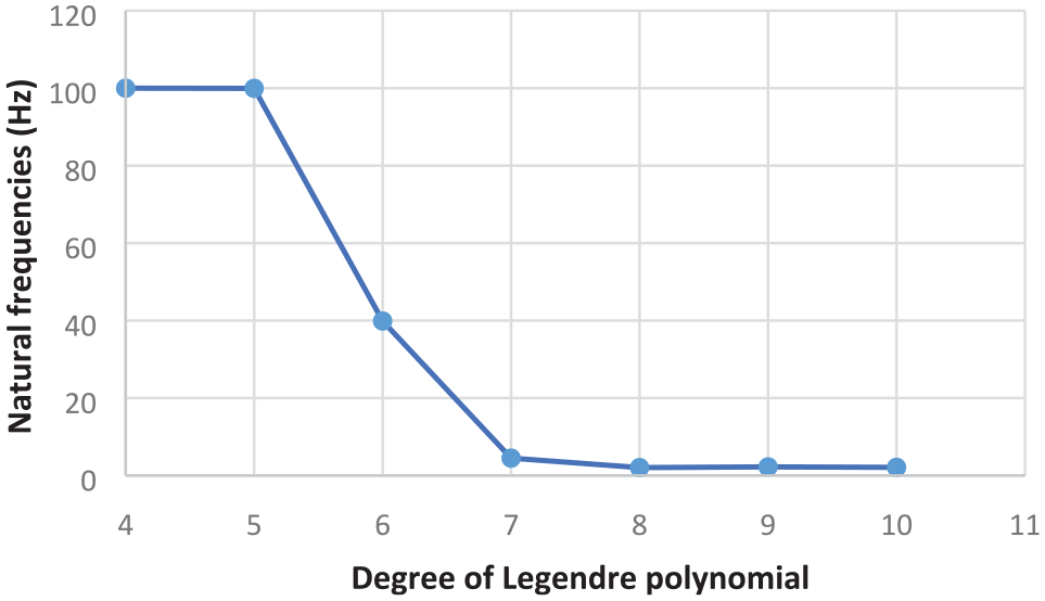
From Tables 1 and 2, we note a perfect agreement with the experimental results by the reference.^43,44 According to Figure 7. We see that the convergence of a polynomial for solid starts with a degree of freedom equal to seven (n = 7) on the other hand, Figure 8. This shows that the convergence of polynomial starts with n = 5, therefore from these results (Figures 7 and 8). We have chosen a degree of freedom of the legendary polynomial n = 8, as an assurance of pressure for the results with different parameters geometric and physical to follow.

We can conclude that the vibration of natural frequencies takes into consideration the geometric and physical parameters. It has also been observed that the frequencies depend on the nature of the circumferential and longitudinal waves. The increase in diameter made it possible to increase the natural frequency of the structure in the absence of fluid, for the boundary conditions and the various circumferential and axial vibratory modes. This means that the rigidity increases by the deformation of the structure. But on the other hand, the presence of the fluid inside the structure gives a significant reduction on the natural frequencies, gives structural stability or the fluid plays a role of a mass adds to structure, can say that the vibratory energy of the structure has been absorbed, by the presence of the fluid, it is additional gain to minimise the frequency energy.

It’s noted that the increase in the thickness of the cylindrical decreases the value of the circumferential natural frequencies of the structure, with or without fluid. In addition, the increase in length implies an increase in natural frequencies for different circumferential and longitudinal modes of the structure.

The goal of this work is to apply the hierarchical finite element method by well-defined polynomials. This method gives a vibratory numerical calculation efficiency of the phenomenon of interaction fluid structure according to the limiting conditions proposed to internal pressure with penalty coupling. The hierarchical finite element method and more precise goat and stable in convergence than other current resolution methods such as finite element methods, by perspective we can study different parameters, turbulence and thermal energy by this HFEM method.

This article presents some important observations based on longitudinal and circumferential vibrations according to which the increase or decrease in natural frequencies follows the nature of the geometric and physical structure obtained in a MATLAB programme, keeping the ratio between the radius on the thickness, the length on the radius, as there is an explanation that the longitudinal frequencies increase rapidly with or without the presence of the fluid and vice versa for the circumferential frequencies, we can say that the importance in all this is of having the ability to control the vibrations to stay in a frequency range sufficiently far from the resonance zone.